Approximating Shepp’s constants for the Slepian process
Abstract
Slepian process is a stationary Gaussian process with zero mean and covariance For any and real , define and the constants and ; we will call them ‘Shepp’s constants’. The aim of the paper is construction of accurate approximations for and hence for the Shepp’s constants. We demonstrate that at least some of the approximations are extremely accurate.
Keywords:
Slepian process, extreme value theory, boundary crossing probability1 Introduction
Let , , be a Gaussian process with mean 0 and covariance
| (1.1) |
This process is often called Slepian process. For any real and , define
| (1.2) |
if we set . Assuming that has Gaussian distribution , and hence the stationarity of the process , we average and thus define
| (1.3) |
where .
Key results on the boundary crossing probabilities for the Slepian process have been established by L.Shepp in [1]. In particular, Shepp has derived an explicit formula for with integer, see (2.5) below. As this explicit formula is quite complicated, in (3.7) in the same paper, Shepp has conjectured the existence of the following constant (depending on )
| (1.4) |
and raised the question of constructing accurate approximations and bounds for this constant.
The importance of this constant is related to the asymptotic relation
| (1.5) |
where . We will call and ‘Shepp’s constants’.
In this paper, we are interested in deriving approximations for in the form (1.5) and hence for the Shepp’s constants. In formulation of approximations, we offer approximations for for all and hence approximations for and . Note that computation of for is a relatively easy problem, see [2] for and [1] for .
In Section 2 we derive several approximations for and and provide numerical results showing that at least some of the derived approximation are extremely accurate. In Section 3 we compare the upper tail asymptotics for the Slepian process and some other stationary Gaussian processes. Section 3 contains some minor technical details and Section 5 delivers conclusions.
2 Construction of approximations
2.1 Existence of Shepp’s constants and the approximations derived from general principles
The fact that the limit in (1.4) exists and hence that is properly defined for any has been proven in [3]. The proof of existence of is based on the inequalities
| (2.1) |
The inequality in the rhs of (2.1) follows directly from the infamous ‘Slepian inequality’ established in [4]; this inequality holds for any Gaussian stationary process with non-negative correlation function. The inequality in the lhs of (2.1) can be obtained by a simple extension of the arguments in [4, p.470]; it holds for any Gaussian stationary process which correlation function vanishes outside the interval . The inequalities (2.1) are not sharp: in particular, for and , (2.1) gives ; see [5, Remark 3]. As follows from Tables 1 and 3, an accurate approximation for is where we claim all four decimal places are accurate.
If is not too small, the bounds (2.1) are very difficult to compute. For small , these bounds are not sharp even if is large, see Fig. 1(a). The bounds improve as grows, see Fig. 1(b). It is not very clear how to use these bounds for construction of accurate approximations for . In particular, from Fig. 1(b) we observe that the upper bound of (2.1) can be much closer to the true than the lower bound.


One may apply general results shown in [6, 7], see also formula in [8], to approximate for large but these results only show that as and therefore are of no use here. A more useful tool, which can be used for approximating , is connected to the following result of J.Pickands proved in [9]. Assume that is a stationary Gaussian random process with , and covariance function
| (2.2) |
and . Then
| (2.3) |
where is the so-called ‘Pickands constant’. By replacing with () and removing the term in (2.3) we obtain a general approximation
| (2.4) |
As shown in [10], the value of the Pickands constant is only known for and hence the approximation (2.4) can only be applied in these cases. When is the Slepian process with covariance function (1.1) we have , and . Hence we obtain from (2.4)
Note that Approximation 0 can also be obtained as a Poisson clumping heuristic, see formula (D10g) in [11]. If is not large, then Approximation 0 is quite poor, see Tables 1 and 2 and Figure 2. For small and moderate values of , the approximations derived below in this section are much superior to Approximation 0.
2.2 Shepp’s formula for
The following formula is the result (2.15) in [1]:
| (2.5) |
where is a positive integer, , L.Shepp in [1] has also derived explicit formulas for with non-integral but these formulas are more complicated and are realistically applicable only for small (say, ).
From (2.5) we straightforwardly obtain
| (2.6) | |||||
| (2.7) |
where . Derivation of explicit formulas for and with is relatively easy as the process is conditionally Markovian in the interval , see [12]. Formula (2.6) has been first derived in [2].
In what follows, also plays a very important role. Using (2.5) and changing the order of integration where suitable, can be expressed through a one-dimensional integral as follows:
| (2.8) | |||||
This expression can be approximated as shown in Appendix; see (4.4).
2.3 An alternative representation of the Shepp’s formula (2.5)
Let be a positive integer, For we set with . It follows from Shepp’s proof of (2.5) that have the meaning of the values of the process at the times : (). The range of the variables is . The variables are expressed via by () with . Changing the variables in (2.5), we obtain
| (2.9) |
where
Expression (2.9) for the probability implies that the function
| (2.11) |
is the joint probability density function for the values under the condition for all .
Since is the value of , the formula (2.11) also shows the transition density from to conditionally for all :
| (2.12) |
For this transition density, .
2.4 Approximating through eigenvalues of integral operators
2.4.1 One-step transition
Let be the largest eigenvalue of the the integral operator with kernel (2.13):
where eigenfunction is some probability density on . The Ruelle-Krasnoselskii-Perron-Frobenius theory of bounded linear positive operators (see e.g. Theorem XIII.43 in [13]) implies that the maximum eigenvalue of the operator with kernel is simple, real and positive and the eigenfunction can be chosen as a probability density.
Similarly to what we have done below in Section 2.4.2, we can suggest computing good numerical approximations to using Gauss-Legendre quadrature formulas. However, we suggest to use (4.15) from [14] instead; this helps us to obtain the following simple but rather accurate approximation to :
2.4.2 Transition in a twice longer interval
Consider now the interval . We could have extended the method of Section 2.4.1 and used the eigenvalue (square root of it) for the transition with transition density expressed in (2.12) with . This would improve Approximation 1 but this improvement is only marginal. Instead, we will use another approach: we consider the transition but use the interval just for setting up the initial condition for observing at .
For , the expression (2.11) for the joint probability density function for the values under the condition for all has the form
Denote by , the ‘non-normalized’ density of under the condition for all that satisfies . Using (2.13), we obtain
Then the transition density from to under the condition for all is achieved by integrating out and renormalising the joint density:
Let be the largest eigenvalue of the integral operator with kernel :
where eigenfunction is some probability density on . Similarly to the case , is simple, real and positive eigenvalue of the operator with kernel and the eigenfunction can be chosen as a probability density.
In numerical examples below we approximate using the methodology described in [15], p.154. It is based on the Gauss-Legendre discretization of the interval , with some large , into an -point set (the ’s are the roots of the -th Legendre polynomial on ), and the use of the Gauss-Legendre weights associated with points ; and are then approximated by the largest eigenvalue and associated eigenvector of the matrix where , and . If is large enough then the resulting approximation to is arbitrarily accurate.
2.4.3 Quality of Approximations 1 and 2
Approximation 1 is more accurate than Approximation 0 but it is still not accurate enough. This is related to the fact that the process is not Markovian and the behaviour of on the interval depends on all values of in the interval and not only on the value , which is a simplification we used for derivation of Approximation 1. Approximation 2 corrects the bias of Approximation 1 by considering twice longer intervals and using the behaviour of in the first half of the interval just for setting up the initial condition at . As shown in Section 2.7, Approximation 2 is much more accurate than Approximations 0 and 1. The approximations developed in the following section also carefully consider the dependence of on its past; they could be made arbitrarily accurate (on expense of increased computational complexity).
2.5 Main approximations
As mentioned above, the behaviour of on the interval depends on all values of in the interval and not only on the value . The exact value of the Shepp’s constant can be defined as the limit (as ) of the probability that for all under the condition for all . Using the formula for conditional probability, we obtain
| (2.17) |
Waiting a long time without reaching is not numerically possible and is not what is really required for computation of . What we need is for the process to (approximately) reach the stationary behaviour in the interval under the condition for all . Since the memory of is short (it follows from the representation , where is the standard Wiener process), this stationary behaviour of is practically achieved for very small , as is seen from numerical results of Section 2.7. Moreover, since ratios are very close to for , we can use ratios in (2.17) instead. Here is the mean of the truncated normal distribution with density , . For computing the approximations, it makes integration easier. Note also another way of justifying the approximation : divide (1.5) with by (1.5) with .
The above considerations give rise to several approximations formulated below. We start with simpler approximations which are easy to compute and end up with approximations which are extremely accurate but are harder to compute. Approximation 7 is very precise, see Table 3. However, we would not recommend extremely accurate Approximations 6 and 7 since Approximations 4 and 5 are already very accurate, see Tables 1 and 2, but are much easier to compute. Approximation 3, the simplest in the family, is also quite accurate. Note that all approximations for can be applied for any .
Numerical complexity of these approximation is related to the necessity of computing either or for suitable . It follows from (2.9) that is an -dimensional integral. Consequently, is an -dimensional integral. In both cases, the dimensionality of the integral can be reduced by one, respectively to and , with no further analytical reduction possible. In view of results of Sections 3 and 4.2, computation of Approximations 3 and 4 is easy, computation of Approximation 5 requires numerical evaluation of a one-dimensional integral (which is not hard) but to compute Approximation 7 we need to approximate a three-dimensional integral, which has to be done with high precision as otherwise Approximation 7 is not worth using: indeed, Approximations 4–6 are almost as good but are much easier to compute. As Approximation 7 provides us with the values which are practically indistinguishable from the true values of , we use Approximation 7 only for the assessment of the accuracy of other approximations and do not recommend using it in practice.
2.6 Consistency of approximations when is large
Assume that . We shall show that Approximations 3-7 for give consistent results with Approximation 0 which is .
Roughly, this consistency follows if we simply use for in (1.5) and then substitute the asymptotically correct values of and in . Similar argument works in the case .
Consider now Approximation 4 for , which is . From explicit formulas (2.7) and (2.8) for and we obtain
| (2.18) | |||||
| (2.19) |
Expansion (2.18) of (2.7) is straightforward. To obtain (2.19) from (2.8) we observe as :
and
all other terms in (2.8) converge to zero (as ) faster than . Using the expansion as , this gives
This is fully consistent with approximation and all the discussion of Section 2.1. However, there is no guarantee that the constant 4 above is the correct constant in the asymptotic relation
provided this asymptotic relation holds.
2.7 Numerical results
In this section we discuss the quality of approximations introduced in Section 2. In Table 1, we present the values of for a number of different ; see also Table 3 in Appendix. As mentioned above, is practically the true and therefore we compare all other approximations against . In Table 2 we present the relative errors of all other approximations against ; that is, the values for . From these two tables we see that Approximations 2-7 are very accurate. Moreover, we have made large-scale simulation studies where we have estimated values of for different using trajectories of and all approximations for considered above. Visually, Approximations 5-7 are virtually exact (the approximations are always well inside the confidence bounds computed from the simulations) for all and also Approximations 2-4 are visually undistinguishable from them for . We do not provide corresponding plots as these plots are not informative.
| =0 | =0.5 | =1 | =1.5 | =2 | =2.5 | =3 | =3.5 | =4 | |
|---|---|---|---|---|---|---|---|---|---|
| | 1.000000 | 0.838591 | 0.785079 | 0.823430 | 0.897644 | 0.957126 | 0.986792 | 0.996950 | 0.999465 |
| | 0.250054 | 0.413754 | 0.596156 | 0.762590 | 0.885025 | 0.955674 | 0.986738 | 0.996958 | 0.999466 |
| | 0.201909 | 0.366973 | 0.563246 | 0.746457 | 0.879719 | 0.954522 | 0.986566 | 0.996939 | 0.999464 |
| | 0.199421 | 0.366664 | 0.564851 | 0.747979 | 0.880220 | 0.954529 | 0.986532 | 0.996930 | 0.999463 |
| | 0.200045 | 0.365730 | 0.562888 | 0.746559 | 0.879831 | 0.954556 | 0.986570 | 0.996939 | 0.999464 |
| | 0.202269 | 0.368099 | 0.564446 | 0.747143 | 0.879943 | 0.954564 | 0.986571 | 0.996939 | 0.999464 |
| | 0.202455 | 0.368100 | 0.564377 | 0.747118 | 0.879945 | 0.954566 | 0.986571 | 0.996939 | 0.999464 |
| | 0.202434 | 0.368082 | 0.564371 | 0.747118 | 0.879945 | 0.954566 | 0.986571 | 0.996939 | 0.999464 |
| =0.5 | =1 | =1.5 | =2 | =2.5 | =3 | =3.5 | =4 | ||
|---|---|---|---|---|---|---|---|---|---|
| | 3.94e+00 | 1.28e+00 | 3.91e-01 | 1.02e-01 | 2.01e-02 | 2.68e-03 | 2.25e-04 | 1.16e-05 | 6.12e-07 |
| | 2.35e-01 | 1.24e-01 | 5.63e-02 | 2.07e-02 | 5.77e-03 | 1.16e-03 | 1.69e-04 | 1.93e-05 | 1.88e-06 |
| | -2.59e-03 | -3.01e-03 | -1.99e-03 | -8.84e-04 | -2.57e-04 | -4.56e-05 | -4.61e-06 | -2.56e-07 | -7.82e-09 |
| | -1.49e-02 | -3.85e-03 | 8.51e-04 | 1.15e-03 | 3.12e-04 | -3.84e-05 | -3.88e-05 | -9.36e-06 | -1.28e-06 |
| | -1.18e-02 | -6.39e-03 | -2.63e-03 | -7.48e-04 | -1.29e-04 | -1.09e-05 | -2.06e-07 | 2.27e-08 | 1.35e-09 |
| | -8.13e-04 | 4.71e-05 | 1.33e-04 | 3.32e-05 | -2.49e-06 | -1.57e-06 | -1.34e-07 | -2.20e-09 | 9.09e-11 |
| | 1.03e-04 | 5.02e-05 | 1.09e-05 | 1.88e-07 | -1.83e-07 | -3.22e-11 | 4.12e-11 | 2.86e-11 | 6.09e-12 |
A plot of the relative errors can be seen in Figure 2(a), where the number next to the line corresponds to the approximation. Approximations 2,4 and 7 suggest very accurate lower bounds for the true . Approximations 0 and 1 appear to provide upper bounds for for all .
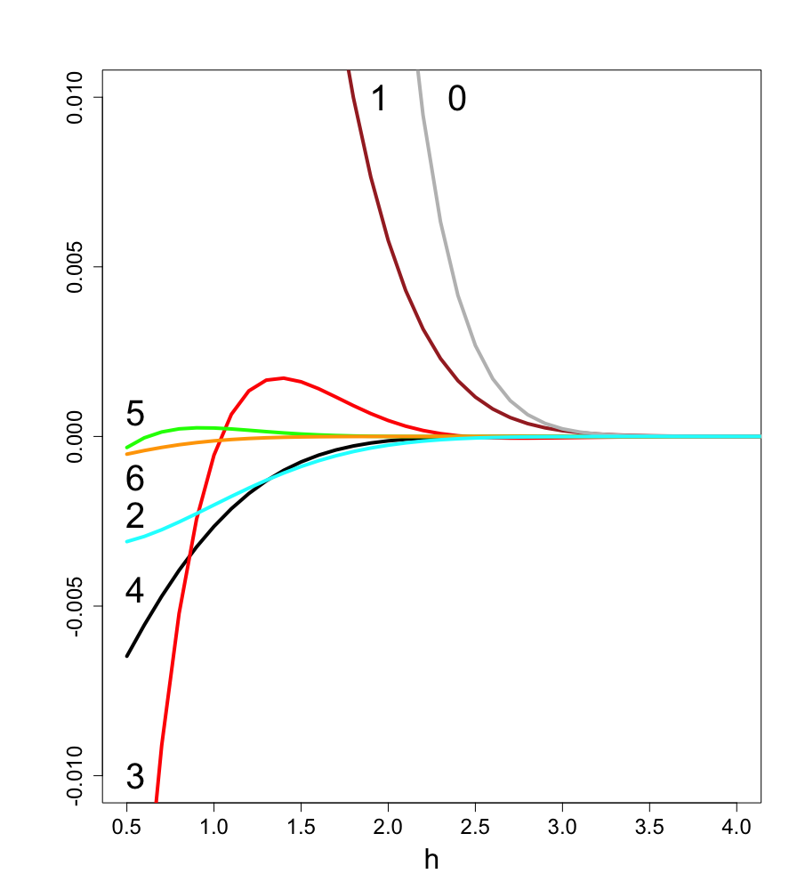

As mentioned in Section 2.4.3, Approximation 1 is not as accurate as Approximations 2–7 because it does not adequately take into account the non-Markovianity of . In Figure 2(b) we have plotted (dotted red line), (dashed red line) and (solid green line) for a range of interesting . Visually, all with would be visually indistinguishable from each other on the plot in Figure 2(b) and would be very close to them. The number next to the line corresponds to which approximation was used.
3 Comparison of the upper tail asymptotics for the Slepian process against some other stationary Gaussian processes
Consider the following three stationary Gaussian processes.
- 1.
() is the Ornstein-Uhlenbeck process with mean 0, variance 1 and correlation function .
- 2.
Let be fixed real number and set . Then, if denotes the standard Wiener process, we define the process () as follows:
The process has mean 0, variance 1 and correlation function
- 3.
Let be a fixed real number and set . Define the process by
The process has mean 0, variance 1 and correlation function
It follows from [12, Theorem 3], the above three processes provide a very good representation of the entire class of conditionally Markov stationary Gaussian processes. Indeed, there is only one process in this class where in (2.2) (this is the process with covariance function with ) and the three types of processes we consider cover well the case where and in (2.2) (the case reduces to the case by substituting for ). For a graphical representation of the chosen covariance functions, see Figure 3(b).
Below we compare Shepp’s constant defined in (1.4) to similar quantities of the processes , () defined above. More precisely, let
We are interested in comparing Shepp’s constant with
| (3.1) |
for Importantly, each process has , and correlation function which satisfies , for .
The existence and evaluation of the constant defined in (3.1) for the Ornstein-Uhlenbeck process has been considered in [16], where it was shown that for all , and that is the root of a parabolic cylinder function (defined in [16]) closest to zero. It is also shown that and . The existence of the constants and follows from similar arguments for the existence of Shepp’s constant . Moreover, the constants are approximated by the same methodology as Shepp’s constant, namely:
| (3.2) |
The justification why we expect (with, say, ) to be a good approximation of is related to the property of ‘fast loss of memory’, which processes and possess, as the process does.
In view of the complex structure of and , the values of and are evaluated via Monte Carlo simulations. In Figure 3(a), we compare with Shepp’s constant (red solid line). (orange dot-dash line) has been computed as in [16] . (blue dashed line) and (dark green dotted line) have been approximated using (3.2) with . For we have taken in the definition of and for we have taken in the definition of . In Figure 3(b), we plot the correlation functions: (red solid line); (orange dot-dash line); (blue dashed line); (dark green dotted line). Note that the results obtained are fully consistent with the celebrated ‘Slepian’s lemma’, a Gaussian comparison inequality, see Lemma 1 in [4]. In our terms, Slepian’s lemma says that if for two stationary Gaussian processes with non-negative covariance functions and we have for all , then for the corresponding values of we have , for all .


4 Appendix
4.1 Approximations for
In Table 3 we use Approximation 7 (our most accurate approximation) to approximate over increments 0.1 for .
Bold font indicates the decimal places which we claim accurate. Note that has been treated as a special case, see for example [4] and
[17]. For , instead of Approximation 7, we have used the approximation ; we do not recommend using this approximation in general because of its high complexity.
| 0.0 | 1.5972 | 0.8 | 0.7240 | 1.6 | 0.250519 | 2.4 | 0.0578944 | 3.2 | 0.0077016 |
| 0.1 | 1.4632 | 0.9 | 0.6450 | 1.7 | 0.213929 | 2.5 | 0.0464986 | 3.3 | 0.0057244 |
| 0.2 | 1.3365 | 1.0 | 0.5720 | 1.8 | 0.181484 | 2.6 | 0.0370122 | 3.4 | 0.0042111 |
| 0.3 | 1.2170 | 1.1 | 0.5051 | 1.9 | 0.152902 | 2.7 | 0.0291909 | 3.5 | 0.0030658 |
| 0.4 | 1.1047 | 1.2 | 0.4438 | 2.0 | 0.127896 | 2.8 | 0.0228058 | 3.6 | 0.0022087 |
| 0.5 | 0.9995 | 1.3 | 0.3879 | 2.1 | 0.106178 | 2.9 | 0.0176462 | 3.7 | 0.0015747 |
| 0.6 | 0.9010 | 1.4 | 0.3372 | 2.2 | 0.087460 | 3.0 | 0.0135203 | 3.8 | 0.0011109 |
| 0.7 | 0.8092 | 1.5 | 0.2915 | 2.3 | 0.071458 | 3.1 | 0.0102561 | 3.9 | 0.0007755 |
4.2 An approximation for
4.3 Simplified form of and its approximation
Using (2.5), for any , we can express as follows:
Using (4.2), we obtain the approximation where
| =0 | =0.5 | =1 | =1.5 | =2 | =2.5 | =3 | =3.5 | =4 | |
|---|---|---|---|---|---|---|---|---|---|
| | 0.041459 | 0.141066 | 0.337112 | 0.588949 | 0.803170 | 0.927924 | 0.979740 | 0.995608 | 0.999264 |
| | 0.041942 | 0.139821 | 0.336115 | 0.588695 | 0.803139 | 0.927922 | 0.979740 | 0.995608 | 0.999264 |
5 Conclusions
In his seminal paper [1], L. Shepp derived explicit formulas for , the distribution of maximum of the so-called Slepian process . As these explicit formulas are complicated, in the same paper L. Shepp has introduced a constant (which we call Shepp’s constant) measuring the rate of decrease of as grows; L. Shepp also raised the question of constructing accurate approximations and bounds for this constant. Until now, this question has not been adequately addressed. To answer it, we have constructed different approximations for (and hence for ). We have shown in Section 2.7 that at least some of these approximations are extremely accurate for all . We have also provided other approximations that are almost as good but are much simpler to compute.
Acknowledgement
The authors are grateful to the AE and both reviewers whose comments much helped for improving the presentation.
References
- [1] L. Shepp. First passage time for a particular Gaussian process. The Annals of Mathematical Statistics, 42(3):946–951, 1971.
- [2] D. Slepian. First passage time for a particular Gaussian process. The Annals of Mathematical Statistics, 32(2):610–612, 1961.
- [3] Wenbo V Li and Qi-Man Shao. Lower tail probabilities for Gaussian processes. The Annals of Probability, 32(1):216–242, 2004.
- [4] D. Slepian. The one-sided barrier problem for Gaussian noise. Bell System Technical Journal, 41(2):463–501, 1962.
- [5] G. Molchan. Survival exponents for some Gaussian processes. International Journal of Stochastic Analysis, 2012.
- [6] H.J. Landau and L.A. Shepp. On the supremum of a Gaussian process. Sankhyā: The Indian Journal of Statistics, Series A, 32:369–378, 1970.
- [7] M. Marcus and L.A. Shepp. Sample behavior of Gaussian processes. In Proc. of the Sixth Berkeley Symposium on Math. Statist. and Prob, 2:423–421, 1972.
- [8] R.J. Adler and J. Taylor. Random Fields and Geometry. Springer, 2007.
- [9] J. Pickands. Upcrossing probabilities for stationary Gaussian processes. Transactions of the American Mathematical Society, 145:51–73, 1969.
- [10] A.J. Harper. Pickands’ constant does not equal , for small . Bernoulli, 23(1):582–602, 2017.
- [11] D. Aldous. Probability Approximations via the Poisson Clumping Heuristic. Springer Science & Business Media, 1989.
- [12] C.B. Mehr and J.A. McFadden. Certain properties of Gaussian processes and their first-passage times. Journal of the Royal Statistical Society. Series B (Methodological), 27(3):505–522, 1965.
- [13] M. Reed and B. Simon. Methods of Modern Mathematical Physics: Scattering theory Vol. 3. Academic Press, 1979.
- [14] J. Noonan and A. Zhigljavsky. Approximations of the boundary crossing probabilities for the maximum of moving sums. arXiv preprint arXiv:1810.09229, 2018.
- [15] J.L. Mohamed and L.M. Delves. Computational Methods for Integral Equations. Cambridge University Press, 1985.
- [16] J.A. Beekman. Asymptotic distributions for the Ornstein-Uhlenbeck process. Journal of Applied Probability, 12(1):107–114, 1975.
- [17] J. Pitman and W. Tang. The Slepian zero set, and Brownian bridge embedded in Brownian motion by a spacetime shift. Electronic Journal of Probability, 20(61):1–28, 2015.
- [18] J.T. Lin. Approximating the normal tail probability and its inverse for use on a pocket calculator. Applied Statistics, 38(1):69–70, 1989.