Hillclimbing inflation in metric and Palatini formulations Preprint: CTPU-18-44Preprint: LDU2018-06Preprint: OU-HET-1002Preprint: UMN–TH–3913/19Preprint: FTPI–MINN–19/04

Cosmic inflation Starobinsky 1980; Guth 1981; Sato 1981 is one of the most important pillars in modern cosmology. It not only solves the flatness and horizon problems Guth 1981 and dilutes possible unwanted relics Sato 1981, but also successfully produces the primordial density perturbations necessary for late-time cosmic structures Mukhanov and Chibisov 1981; Kodama and Sasaki 1984. Cosmic microwave background (CMB) observations have been contributing to narrow down inflationary models (e.g. Ref. Akrami et al. 2018), and further improvement in the experimental sensitivity is expected in the future Matsumura et al. 2013; Inoue et al. 2016; Delabrouille et al. 2017.

As the observational constraints become more stringent, there have been growing interests in the attractors of inflation models. One of the well-known attractors is inflation with the $R^{2}$ term Starobinsky 1980, which realizes inflation through a modification of the gravitational action. Another well known example is the inflation with nonminimal coupling, which has been studied from 80’s Lucchin et al. 1986; Futamase and Maeda 1989; Salopek et al. 1989; Fakir and Unruh 1990; Makino and Sasaki 1991; van der Bij 1994; van der Bij 1995; Park and Yamaguchi 2008, and been more extensively studied after Higgs inflation Salopek et al. 1989; Cervantes-Cota and Dehnen 1995 became one of the main topics in modern particle cosmology Bezrukov and Shaposhnikov 2008; Hamada et al. 2014; Hamada et al. 2015; He et al. 2019.^aa a The setup can be generalized to a requirement that $V_{\text{J}}/\Omega^{2}$ approaches a constant value at the range of inflation Park and Yamaguchi 2008. These attractor-type models enjoy their inflationary predictions well within the observational sweet spot. Such attractor models have been generalized to the $\alpha$-attractor Kallosh et al. 2013. In this context, a systematic study of small conformal-factor attractor has been proposed in Ref. Jinno and Kaneta 2017, and as a result a new realization of Higgs inflation has been discovered Jinno et al. 2018.

In this paper we introduce a new attractor setup in the context of hillclimbing inflation. The model consists of periodic conformal factor (i.e. scalar field coupling to the Ricci scalar) and potential, but it still enjoys the attractor-type inflationary predictions. One of the interesting features of the model is that it predicts the observationally favored values of inflationary observables both in the metric and the Palatini formulations of gravity Palatini 1919; Einstein 1925.^bb b The paper Palatini 1919 by Palatini is often referred to for the Palatini formulation, but it is reported Ferraris et al. 1982 that the formulation was introduced in the paper Einstein 1925 by Einstein. The Palatini formulation, where the connection $\Gamma$ is regarded as another independent variable to take variation with in addition to the metric $g$, has been known as a formulation of gravity distinctive from the metric formulation, in which $\Gamma(g)$ is set to be the Levi-Civita connection and is given as a function of $g$. Though these two formulations give the identical predictions as long as we consider the pure Einstein gravity and minimally-coupled matter fields, it is known that they lead to different dynamics once gravity action is modified or nontrivial couplings between gravity and matter are introduced. This difference has been attracting considerable attention recently Bauer and Demir 2008; Bauer and Demir 2011; Rasanen and Wahlman 2017; Tenkanen 2017; Racioppi 2017; Racioppi 2018; Antoniadis et al. 2018; Carrilho et al. 2018; Enckell et al. 2018a; Enckell et al. 2018b; Jrv et al. 2018; Markkanen et al. 2018; Rasanen and Tomberg 2018; Rasanen 2018; Takahashi and Tenkanen 2018, especially in the context of Higgs inflation.

The organization of the paper is as follows. First we introduce our setup in Sec. II where the inflationary predictions are analytically investigated both in the metric and the Palatini formulations. Next we present numerical results in Sec. III. We finally conclude in Sec. IV.

The setup we consider in this paper is

$\displaystyle S$

$\displaystyle=\int d^{4}x\sqrt{-g_{\text{J}}}\left[\frac{1}{2}\Omega R_{\text{J}}-\frac{\kappa}{2}g_{\text{J}}^{\mu\nu}\partial_{\mu}\phi_{\text{J}}\partial_{\nu}\phi_{\text{J}}-V_{\text{J}}(\phi_{\text{J}})\right],$

(1)

with the ‘‘natural inflation’’-type potential^cc c Note that the potential (3) is realized for example as the difference of two $\cos$-type potentials: $\displaystyle\sin^{4}(\phi_{\text{J}}/f)$ $\displaystyle=\frac{1-\cos(2\phi_{\text{J}}/f)}{2}-\frac{1-\cos(4\phi_{\text{J}}/f)}{8}.$ (2) This type of potential has been used for example in Ref. Czerny et al. 2014, and its UV completion has been discussed for example in Ref. Czerny and Takahashi 2014. As will become clear in the following discussion, $V_{\text{J}}$ needs to behave as $\phi_{\text{J}}^{4}$ around a potential minimum in order for inflation to occur in the Palatini formulation.

$\displaystyle V_{\text{J}}$

$\displaystyle=\Lambda^{4}\sin^{4}\left(\frac{\phi_{\text{J}}}{f}\right).$

(3)

We adopt the Planck unit $M_{\text{P}}\equiv 1/\sqrt{8\pi G}=1$ (with $G$ being the Newtonian constant) throughout the paper. Also, the subscript ‘‘J” refers to the Jordan frame. The main purpose of the present paper is to point out that this type of potential predicts the observationally allowed region with the following choice of the conformal factor:^dd d The form of $\Omega$ is chosen from phenomenological requirement $V_{\text{J}}/\Omega^{2}\to\text{const.}$ at a point of $V_{\text{J}}=0$ as discussed in Ref. Jinno and Kaneta 2017. The existence of coincident zero of $\Omega$ with the $V_{\text{J}}=0$ point is motivated by the generalized multiple-point principle: this model fits into the class of “new” version of MPP corresponding to the weak energy condition Oda.

$\displaystyle\Omega$

$\displaystyle=\omega\sin^{2}\left(\frac{\phi_{\text{J}}}{\eta f}\right).$

(4)

The normalization constant $\omega=1/\sin^{2}(\pi/\eta)$ is fixed to give a proper value of gravitational interaction $\Omega=1$ at the minimum of the potential $\phi_{\text{J}}=\pi f$, and $\eta$ is a real free parameter controlling the ratio between the period of the potential ($2\pi f$) and that of the conformal factor ($2\pi\eta f$). We further impose $\eta>1$ in order for inflation to successfully end at the potential minimum. Also, because of the subtleties discussed in Appendix A, we further restrict $\eta$ to be $\eta\geq 2$. The results for $1<\eta<2$ are explained in this appendix.

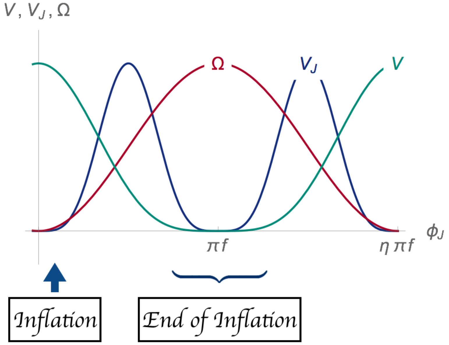
The setup is summarized in Fig. 1. As we will see later, one of the interesting features of the present setup is that it predicts the observationally allowed region both in the metric and Palatini formulations of gravity. Also, for the metric formulation, the existence of the kinetic term in the action (1) is not even mandatory to achieve successful inflation. Therefore we consider both $\kappa=0$ and $\kappa=1$ for the metric case, while we exclusively take $\kappa=1$ for the Palatini case.

In the following discussion, we redefine the metric:

$\displaystyle g_{\mu\nu}$

$\displaystyle=\Omega g_{\text{J}\mu\nu}.$

(5)

This gives the transformation law of the Ricci scalar, which depends on the choice of the formulation. It also gives the relation between the original inflaton $\phi_{\text{J}}$ and the canonical inflaton $\phi$ after the redefinition. The resulting Einstein-frame action becomes

$\displaystyle S$

$\displaystyle=\int d^{4}x\sqrt{-g}\left[\frac{1}{2}R-\frac{1}{2}(\partial\phi)^{2}-V(\phi)\right],$

(6)

with $(\partial\phi)^{2}\equiv g^{\mu\nu}\partial_{\mu}\phi\partial_{\nu}\phi$. The Einstein-frame potential $V$ in terms of the original inflaton $\phi_{\text{J}}$ becomes

$\displaystyle V$

$\displaystyle=\frac{V_{\text{J}}}{\Omega^{2}}=\frac{\Lambda^{4}\sin^{4}(\phi_{\text{J}}/f)}{\omega^{2}\sin^{4}(\phi_{\text{J}}/\eta f)}.$

(7)

This is one of the hillclimbing setups Jinno and Kaneta 2017, namely, around $\phi_{\text{J}}=0$, the potential behaves like $V_{\text{J}}\propto\phi_{\text{J}}^{4}$ while the conformal factor behaves like $\Omega\propto\phi_{\text{J}}^{2}$. As a result, as we see from Fig. 1, the potential minimum around $\phi_{\text{J}}=0$ is no more a minimum in the Einstein frame. At the same time, the relation between the Jordan and Einstein frame inflatons gives an exponential stretching in the canonical field in the latter frame. Here the relation between the original and new inflatons $\phi_{\text{J}}$ and $\phi$ depends on the formulation of gravity and the choice of the kinetic term $\kappa$. As a result, our basic scenario is as follows:

• •

  First, inflation occurs around $\phi_{\text{J}}=+0$ (corresponding to $\phi=\infty$), which is no more a minimum but a maximum in the Einstein frame.

• •

  Next, the inflaton rolls down to the minimum $\phi_{\text{J}}=\pi f$ (corresponding to $\phi=0$), where the inflation ends.

The slow-roll parameters and $e$-folding are calculated in terms of the original inflaton as

	$\displaystyle\epsilon_{V}$	$\displaystyle\equiv\frac{1}{2}\left(\frac{dV/d\phi}{V}\right)^{2}=\frac{1}{2}\left(\frac{dV/d\phi_{\text{J}}}{V}\right)^{2}\frac{1}{(d\phi/d\phi_{\text{J}})^{2}},$		(8)
	$\displaystyle\eta_{V}$	$\displaystyle\equiv\frac{d^{2}V/d\phi^{2}}{V}$
		$\displaystyle=\left[\frac{d^{2}V/d\phi_{\text{J}}^{2}}{V}\frac{1}{(d\phi/d\phi_{\text{J}})^{2}}-\frac{dV/d\phi_{\text{J}}}{V}\frac{d^{2}\phi/d\phi_{\text{J}}^{2}}{(d\phi/d\phi_{\text{J}})^{3}}\right],$		(9)
	$\displaystyle N$	$\displaystyle=\int\frac{d\phi}{\sqrt{2\epsilon_{V}}}=\int\frac{d\phi_{\text{J}}}{d\ln V/d\phi_{\text{J}}}\left(\frac{d\phi}{d\phi_{\text{J}}}\right)^{2}.$		(10)

We take the lower end of the integration to be $\phi=0$ so that $N=0$ at $\phi=0$.^ee e Note that the difference between this definition and the usual definition $N=0$ at $\max(|\epsilon_{V}|,|\eta_{V}|)=1$ gives only next-leading corrections in $N$ to the inflationary predictions.

The inflationary predictions become

$\displaystyle{\mathcal{P}}_{\zeta}$

$\displaystyle\simeq\frac{1}{24\pi^{2}}\frac{V}{\epsilon_{V}},~~~~n_{s}\simeq 1-6\epsilon_{V}+2\eta_{V},~~~~r\simeq 16\epsilon_{V}.$

(11)

In the following analysis we fix ${\mathcal{P}}_{\zeta}=2.1\times 10^{-9}$ Akrami et al. 2018. This gives the overall height of the potential $\propto\Lambda^{4}$ as a function of $f$ for each setup. In the following we examine the metric and the Palatini formulations one by one.

In this section we present numerical results for the inflationary predictions in the setup explained in the previous section, and also discuss possible reheating processes.

Figures 4 and 5 are the inflationary predictions of the setup (1). The former is for $\eta=2$ (left panel) and $3$ (right panel), while the latter is for $\eta=10$. The lines starting from the smiley markers and ending at the blue stars (from $f=10^{2}M_{\text{P}}$ to $f=10^{-1}M_{\text{P}}$) are for the metric formulation with the kinetic term ($\kappa=1$). The left and right lines correspond to $N=50$ and $60$, respectively. The value of $f$ is also indicated in color.

We see that, for the metric formulation, the prediction is the same as that of the quartic chaotic inflation (smiley markers) for larger $f$ ($\gtrsim 1$), while it approaches to the attractor points (stars) for smaller $f$ ($\lesssim 1$). For the metric formulation without the kinetic term ($\kappa=0$), the prediction is $f$-independent and always comes at the position of the stars. We also note that their positions are almost $\eta$-independent, as seen from the leading-order predictions (19).

On the other hand, the lines going into the $r\ll 1$ region are for the Palatini formulation. The prediction is again the same as that of the quartic chaotic inflation for larger $f$ ($\gtrsim 1$), while it behaves differently from the metric case for smaller $f$ ($\lesssim 1$). This behavior can be understood from Eq. (27), and therefore we see that, if $r$ is observationally found to much smaller than $10^{-2}$, the Palatini formulation can provide a better fit to the data. We also see that the prediction with $f=\sqrt{6}/\pi$ in the Palatini formulation coincides with that of the metric formulation for $\eta\gg 1$.

Before moving on to conclusions, we comment on possible reheating mechanisms. First, preheating Kofman et al. 1994; Kofman et al. 1997 is very likely to occur in the current setup. However, as expected from earlier studies, the dynamics is highly sensitive to (1) the existence of the kinetic term in the original frame Ema et al. 2017, (2) the existence of other degrees of freedom (e.g. whether the inflaton is real or complex Bezrukov et al. 2009; Garcia-Bellido et al. 2009; Ema et al. 2017, or whether the scalaron degree of freedom exists or not Ema 2017; He et al. 2018; He et al. 2019), (3) the choice of formulations Rubio and Tomberg 2019, and so on. All of these need further investigation, but are beyond the scope of the present paper. Second, reheating via the perturbative inflaton decay can be implemented in both metric and Palatini formulations. In the current setup the inflaton actually becomes massless at the potential minimum in both formulations, and thus perturbative inflaton decay does not occur.^hh h This can be seen as the inflaton mass $m_{\phi}$ is given by $\displaystyle m_{\phi}^{2}$ $\displaystyle=K\left(\frac{\partial K}{\partial\phi_{\text{J}}}\frac{\partial V_{\text{J}}}{\partial\phi_{\text{J}}}+K\frac{\partial^{2}V_{\text{J}}}{\partial\phi_{\text{J}}^{2}}\right),$ with $K(\phi_{\text{J}})\equiv d\phi_{\text{J}}/d\phi$, and $\partial V_{\text{J}}/\partial\phi_{\text{J}}=\partial^{2}V_{\text{J}}/\partial\phi_{\text{J}}^{2}=0$ at $\phi_{\text{J}}=\pi f$. Note that this is valid except for $\eta=2$ in the $\kappa=0$ case. A remedy may be to incorporate a coupling to the SM Higgs field $H$. For instance, if we modify the Jordan-frame potential to include

$\displaystyle V_{\text{J}}$

$\displaystyle\supset\lambda\Lambda^{2}|H|^{2}\sin^{2}(\phi_{\text{J}}/f),$

(28)

with a certain coupling $\lambda$, the inflaton acquires a mass $m_{\phi}\sim\lambda\Lambda\langle H\rangle/f$ once the inflation ends and the electroweak symmetry is broken, whereas during inflation the Higgs is stabilized at the origin by this coupling and thus the inflaton dynamics would be kept intact.ⁱⁱ i The inflaton mass thus induced may fall within the reach of low energy experiments such as the ones searching for Axion-like particle or dark photons. Further details are reserved for future study. Once the inflaton acquires a heavier mass than the Higgs, the reheating may take place by the inflaton decay into Higgs bosons. Even if the tree-level decay is kinematically forbidden, the inflaton can decay into a pair of lighter SM particles through the Higgs loop diagrams.

In this paper we discussed a new realization of cosmic inflation where both the inflaton potential and conformal factor are periodic functions of the inflaton field. In particular, we focused on the realization both in the metric and Palatini formulations of gravity, adopting a specific type of the potential and conformal factor, namely, sinusoidal functions as a variant possibility of natural inflation. We showed that our setup gives inflationary predictions well consistent with cosmic microwave background observations in both formulations. We also argued that, for the metric formulation case, the existence of the kinetic term in the Jordan frame is not mandatory, and the consistent predictions can be obtained. Future observations, particularly those sensitive to $r={\cal O}(10^{-3})$, may be able to distinguish between the metric and the Palatini formulations in our setup Matsumura et al. 2013; Inoue et al. 2016; Delabrouille et al. 2017.

The work of RJ was supported by IBS under the project code, IBS-R018-D1. The work of SP was supported in part by the National Research Foundation of Korea (NRF) grant funded by the Korean government (MSIP) (No. 2016R1A2B2016112) and (NRF-2018R1A4A1025334). The work of KK was supported in part by the DOE grant DE–SC0011842 at the University of Minnesota.

References

- Starobinsky (1980) Alexei A. Starobinsky, “A New Type of Isotropic Cosmological Models Without Singularity,” Phys. Lett. B91, 99–102 (1980).
- Guth (1981) Alan H. Guth, “The Inflationary Universe: A Possible Solution to the Horizon and Flatness Problems,” Phys. Rev. D23, 347–356 (1981).
- Sato (1981) K. Sato, “First Order Phase Transition of a Vacuum and Expansion of the Universe,” Mon. Not. Roy. Astron. Soc. 195, 467–479 (1981).
- Mukhanov and Chibisov (1981) Viatcheslav F. Mukhanov and G. V. Chibisov, “Quantum Fluctuations and a Nonsingular Universe,” JETP Lett. 33, 532–535 (1981), [Pisma Zh. Eksp. Teor. Fiz.33,549(1981)].
- Kodama and Sasaki (1984) Hideo Kodama and Misao Sasaki, “Cosmological Perturbation Theory,” Prog. Theor. Phys. Suppl. 78, 1–166 (1984).
- Akrami et al. (2018) Y. Akrami et al. (Planck), “Planck 2018 results. X. Constraints on inflation,” (2018), arXiv:1807.06211 [astro-ph.CO] .
- Matsumura et al. (2013) T. Matsumura et al., “Mission design of LiteBIRD,” (2013), 10.1007/s10909-013-0996-1, [J. Low. Temp. Phys.176,733(2014)], arXiv:1311.2847 [astro-ph.IM] .
- Inoue et al. (2016) Y. Inoue et al. (POLARBEAR), “POLARBEAR-2: an instrument for CMB polarization measurements,” Proceedings, SPIE Astronomical Telescopes + Instrumentation 2016 : Millimeter, Submillimeter, and Far-Infrared Detectors and Instrumentation for Astronomy VIII: Edinburgh, United Kingdom, June 28-July 1, 2016, Proc. SPIE Int. Soc. Opt. Eng. 9914, 99141I (2016), arXiv:1608.03025 [astro-ph.IM] .
- Delabrouille et al. (2017) J. Delabrouille et al. (CORE), “Exploring Cosmic Origins with CORE: Survey requirements and mission design,” (2017), arXiv:1706.04516 [astro-ph.IM] .
- Lucchin et al. (1986) F. Lucchin, S. Matarrese, and M. D. Pollock, “Inflation With a Nonminimally Coupled Scalar Field,” Phys. Lett. B167, 163 (1986).
- Futamase and Maeda (1989) T. Futamase and Kei-ichi Maeda, “Chaotic Inflationary Scenario in Models Having Nonminimal Coupling With Curvature,” Phys. Rev. D39, 399–404 (1989).
- Salopek et al. (1989) D. S. Salopek, J. R. Bond, and James M. Bardeen, “Designing Density Fluctuation Spectra in Inflation,” Phys. Rev. D40, 1753 (1989).
- Fakir and Unruh (1990) R. Fakir and W. G. Unruh, “Improvement on cosmological chaotic inflation through nonminimal coupling,” Phys. Rev. D41, 1783–1791 (1990).
- Makino and Sasaki (1991) Nobuyosi Makino and Misao Sasaki, “The Density perturbation in the chaotic inflation with nonminimal coupling,” Prog. Theor. Phys. 86, 103–118 (1991).
- van der Bij (1994) J. J. van der Bij, “Can gravity make the Higgs particle decouple?” Acta Phys. Polon. B25, 827–832 (1994), hep-th/9310064 .
- van der Bij (1995) J. J. van der Bij, “Can gravity play a role at the electroweak scale?” Int. J. Phys. 1, 63 (1995), arXiv:hep-ph/9507389 [hep-ph] .
- Park and Yamaguchi (2008) Seong Chan Park and Satoshi Yamaguchi, “Inflation by non-minimal coupling,” JCAP 0808, 009 (2008), arXiv:0801.1722 [hep-ph] .
- Cervantes-Cota and Dehnen (1995) Jorge L. Cervantes-Cota and H. Dehnen, “Induced gravity inflation in the standard model of particle physics,” Nucl. Phys. B442, 391–412 (1995), arXiv:astro-ph/9505069 [astro-ph] .
- Bezrukov and Shaposhnikov (2008) Fedor L. Bezrukov and Mikhail Shaposhnikov, “The Standard Model Higgs boson as the inflaton,” Phys. Lett. B659, 703–706 (2008), arXiv:0710.3755 [hep-th] .
- Hamada et al. (2014) Yuta Hamada, Hikaru Kawai, Kin-ya Oda, and Seong Chan Park, “Higgs Inflation is Still Alive after the Results from BICEP2,” Phys. Rev. Lett. 112, 241301 (2014), arXiv:1403.5043 [hep-ph] .
- Hamada et al. (2015) Yuta Hamada, Hikaru Kawai, Kin-ya Oda, and Seong Chan Park, “Higgs inflation from Standard Model criticality,” Phys. Rev. D91, 053008 (2015), arXiv:1408.4864 [hep-ph] .
- He et al. (2019) Minxi He, Ryusuke Jinno, Kohei Kamada, Seong Chan Park, Alexei A. Starobinsky, and Jun’ichi Yokoyama, “On the violent preheating in the mixed Higgs- inflationary model,” Phys. Lett. B791, 36–42 (2019), arXiv:1812.10099 [hep-ph] .
- Kallosh et al. (2013) Renata Kallosh, Andrei Linde, and Diederik Roest, “Superconformal Inflationary -Attractors,” JHEP 11, 198 (2013), arXiv:1311.0472 [hep-th] .
- Jinno and Kaneta (2017) Ryusuke Jinno and Kunio Kaneta, “Hill-climbing inflation,” Phys. Rev. D96, 043518 (2017), arXiv:1703.09020 [hep-ph] .
- Jinno et al. (2018) Ryusuke Jinno, Kunio Kaneta, and Kin-ya Oda, “Hill-climbing Higgs inflation,” Phys. Rev. D97, 023523 (2018), arXiv:1705.03696 [hep-ph] .
- Palatini (1919) Attilio Palatini, “Deduzione invariantiva delle equazioni gravitazionali dal principio di hamilton,” Rendiconti del Circolo Matematico di Palermo (1884-1940) 43, 203–212 (1919).
- Einstein (1925) Albert Einstein, “Einheitliche feldtheorie von gravitation und elektrizität,” Verlag der Koeniglich-Preussichen Akademie der Wissenschaften 22, 414–419 (1925).
- Ferraris et al. (1982) M. Ferraris, M. Francaviglia, and C. Reina, “Variational formulation of general relativity from 1915 to 1925 “palatini’s method” discovered by einstein in 1925,” General Relativity and Gravitation 14, 243–254 (1982).
- Bauer and Demir (2008) Florian Bauer and Durmus A. Demir, “Inflation with Non-Minimal Coupling: Metric versus Palatini Formulations,” Phys. Lett. B665, 222–226 (2008), arXiv:0803.2664 [hep-ph] .
- Bauer and Demir (2011) Florian Bauer and Durmus A. Demir, “Higgs-Palatini Inflation and Unitarity,” Phys. Lett. B698, 425–429 (2011), arXiv:1012.2900 [hep-ph] .
- Rasanen and Wahlman (2017) Syksy Rasanen and Pyry Wahlman, “Higgs inflation with loop corrections in the Palatini formulation,” JCAP 1711, 047 (2017), arXiv:1709.07853 [astro-ph.CO] .
- Tenkanen (2017) Tommi Tenkanen, “Resurrecting Quadratic Inflation with a non-minimal coupling to gravity,” JCAP 1712, 001 (2017), arXiv:1710.02758 [astro-ph.CO] .
- Racioppi (2017) Antonio Racioppi, “Coleman-Weinberg linear inflation: metric vs. Palatini formulation,” JCAP 1712, 041 (2017), arXiv:1710.04853 [astro-ph.CO] .
- Racioppi (2018) Antonio Racioppi, “New universal attractor in nonminimally coupled gravity: Linear inflation,” Phys. Rev. D97, 123514 (2018), arXiv:1801.08810 [astro-ph.CO] .
- Antoniadis et al. (2018) I. Antoniadis, A. Karam, A. Lykkas, and K. Tamvakis, “Palatini inflation in models with an term,” (2018), arXiv:1810.10418 [gr-qc] .
- Carrilho et al. (2018) Pedro Carrilho, David Mulryne, John Ronayne, and Tommi Tenkanen, “Attractor Behaviour in Multifield Inflation,” JCAP 1806, 032 (2018), arXiv:1804.10489 [astro-ph.CO] .
- Enckell et al. (2018a) Vera-Maria Enckell, Kari Enqvist, Syksy Rasanen, and Lumi-Pyry Wahlman, “Inflation with term in the Palatini formalism,” (2018a), arXiv:1810.05536 [gr-qc] .
- Enckell et al. (2018b) Vera-Maria Enckell, Kari Enqvist, Syksy Rasanen, and Eemeli Tomberg, “Higgs inflation at the hilltop,” JCAP 1806, 005 (2018b), arXiv:1802.09299 [astro-ph.CO] .
- Jrv et al. (2018) Laur Jrv, Antonio Racioppi, and Tommi Tenkanen, “Palatini side of inflationary attractors,” Phys. Rev. D97, 083513 (2018), arXiv:1712.08471 [gr-qc] .
- Markkanen et al. (2018) Tommi Markkanen, Tommi Tenkanen, Ville Vaskonen, and Hardi Veermäe, “Quantum corrections to quartic inflation with a non-minimal coupling: metric vs. Palatini,” JCAP 1803, 029 (2018), arXiv:1712.04874 [gr-qc] .
- Rasanen and Tomberg (2018) Syksy Rasanen and Eemeli Tomberg, “Planck scale black hole dark matter from Higgs inflation,” (2018), arXiv:1810.12608 [astro-ph.CO] .
- Rasanen (2018) Syksy Rasanen, “Higgs inflation in the Palatini formulation with kinetic terms for the metric,” (2018), arXiv:1811.09514 [gr-qc] .
- Takahashi and Tenkanen (2018) Tomo Takahashi and Tommi Tenkanen, “Towards distinguishing variants of non-minimal inflation,” (2018), arXiv:1812.08492 [astro-ph.CO] .
- Czerny et al. (2014) Michael Czerny, Tetsutaro Higaki, and Fuminobu Takahashi, “Multi-Natural Inflation in Supergravity,” JHEP 05, 144 (2014), arXiv:1403.0410 [hep-ph] .
- Czerny and Takahashi (2014) Michael Czerny and Fuminobu Takahashi, “Multi-Natural Inflation,” Phys. Lett. B733, 241–246 (2014), arXiv:1401.5212 [hep-ph] .
- (46) Kin-ya Oda, “A generalized multiple-point (criticality) principle and inflation,” in workshop “Scale invariance in particle physics and cosmology,” 28 Janunary–1 February 2019, CERN; https://indico.cern.ch/event/740038/contributions/3283934/ .
- Kofman et al. (1994) Lev Kofman, Andrei D. Linde, and Alexei A. Starobinsky, “Reheating after inflation,” Phys. Rev. Lett. 73, 3195–3198 (1994), arXiv:hep-th/9405187 [hep-th] .
- Kofman et al. (1997) Lev Kofman, Andrei D. Linde, and Alexei A. Starobinsky, “Towards the theory of reheating after inflation,” Phys. Rev. D56, 3258–3295 (1997), arXiv:hep-ph/9704452 [hep-ph] .
- Ema et al. (2017) Yohei Ema, Ryusuke Jinno, Kyohei Mukaida, and Kazunori Nakayama, “Violent Preheating in Inflation with Nonminimal Coupling,” JCAP 1702, 045 (2017), arXiv:1609.05209 [hep-ph] .
- Bezrukov et al. (2009) F. Bezrukov, D. Gorbunov, and M. Shaposhnikov, “On initial conditions for the Hot Big Bang,” JCAP 0906, 029 (2009), arXiv:0812.3622 [hep-ph] .
- Garcia-Bellido et al. (2009) Juan Garcia-Bellido, Daniel G. Figueroa, and Javier Rubio, “Preheating in the Standard Model with the Higgs-Inflaton coupled to gravity,” Phys. Rev. D79, 063531 (2009), arXiv:0812.4624 [hep-ph] .
- Ema (2017) Yohei Ema, “Higgs Scalaron Mixed Inflation,” Phys. Lett. B770, 403–411 (2017), arXiv:1701.07665 [hep-ph] .
- He et al. (2018) Minxi He, Alexei A. Starobinsky, and Jun’ichi Yokoyama, “Inflation in the mixed Higgs- model,” JCAP 1805, 064 (2018), arXiv:1804.00409 [astro-ph.CO] .
- Rubio and Tomberg (2019) Javier Rubio and Eemeli S. Tomberg, “Preheating in Palatini Higgs inflation,” (2019), arXiv:1902.10148 [hep-ph] .