Secure Modulo Sum via Multiple Access Channel Thanks: The work reported here was supported in part by Guangdong Provincial Key Laboratory (Grant No. 2019B121203002), the JSPS Grant-in-Aid for Scientific Research (A) No.17H01280, (B) No. 16KT0017, and Kayamori Foundation of Informational Science Advancement.

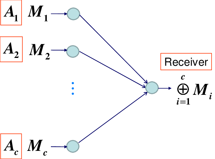
Recently, secure multiparty computation has been actively studied even from the information theoretical viewpoint. One of its simple examples is secure computation of modular sum [1, 2]. This problem has been often discussed from the Shannon-theoretic viewpoint [3, 4]. If we assume secure communication channels between a part of players, secure computation of modular sum is possible. Secure communication channels consumes cryptographic resources. In this paper, instead of such resources, we focus on multiple access channel (MAC), which has been actively studied for a long time [5, 6, 7]. That is, we study how to realize secure computation via MAC instead of conventional secure communication channels. As a typical example, we investigate secure computation of modular sum when a MAC from distinct players $A_{1},\ldots,A_{c}$ to a third party (Receiver) is given. That is, each player $A_{i}$ sends a sequence of their secure random number $M_{i}=(M_{i,1},\ldots,M_{i,k})\in\mathbb{F}_{q}^{k}$ that is subject to the uniform distribution, and Receiver recovers only the modulo sums $M_{[c]}:=(\oplus_{i=1}^{c}M_{i,1},\ldots,\oplus_{i=1}^{c}M_{i,k})$ as Fig. 1, where $\oplus_{i=1}^{c}M_{i,1}:=M_{1,j}\oplus\cdots\oplus M_{c,j}$ and $[c]:=\{1,\ldots,c\}$. Here, to keep the secrecy, it is required that Receiver cannot obtain any information except for the modulo sums. In this way, we can compute the modulo sums. As a simple case [8, 9], we may consider the channel where the output signal $Y$ of the channel is given as

with the $i$-th input variables $X_{i}$ and the noise variable $N$, where $\oplus$ is the modulo sum.

When all senders encode their message by using the same linear code, the receiver cannot obtain any information with respect to each sender’s message because each message is subject to the uniform distribution. Hence, the code is decodable under the noise $N$, the receiver can recover the modulo sums $(\oplus_{i=1}^{c}M_{i,1},\ldots,\oplus_{i=1}^{c}M_{i,k})$. However, the real channel does not has such a form. A realistic example is a Gaussian MAC, whose typical case is given as follows. The receiving signal $Y$ takes values in the set of real numbers $\mathbb{R}$, and the $i$-th sender’s signal $X_{i}$ takes values in discrete values $\{0,1,\ldots,p-1\}$. Then, a typical channel is given as

where $E$ is a constant and $N$ is the Gaussian variable with average 0 and variance $v$. In this case, a part of information for the message of each sender might be leaked to the receiver. To cover Gaussian MAC, this paper addresses a general MAC.

If the secrecy condition is not imposed and the channel is a Gaussian MAC, this problem is a simple example of computation-and-forward [10, 11, 12, 13, 14, 15, 16, 17]. Due to the secrecy condition, we cannot realize this task by their simple application. In the case of $c=2$, since the modulo sums give the information of the other player, the protocol enables the two players to exchange their messages without information leakage to Receiver [18, 19, 20, 21, 22, 23] when Receiver broadcasts the modulo sum to both players. Application of such a protocol is discussed in several network models [26]. Our protocol can be regarded as an multi-player extension with a generic setting of the protocol given in [18, 19, 20, 21, 22, 23].

Further, when we can realize secure transmission of modulo sum with $k$ transmitter, multiplying $-1$ to the receiver’s variable, we can realize secure modulo zero-sum randomness among $k+1$ players, that is the $k+1$ random variables with zero-sum condition and certain security conditions [24, Section 2][25, Section II]. As is explained in [24, 25], secure modulo zero-sum randomness can be regarded as a cryptographic resource for several cryptographic tasks including secure multi-party computation of homomorphic functions, secret sharing without secure communication channel, and a cryptographic task, multi-party anonymous authentication. In this sense, secure transmission of modulo sum is needed in the viewpoint of cryptography.

In this paper, we formulate the secure modulo sum capacity as the maximum of the secure transmission of modulo sum via multiple access channel. When the multiple access channel satisfies a symmetric condition, the secure modulo sum capacity equals the capacity of a certain single access channel. In a general setting, we derive the lower bound of the secure modulo sum capacity. Further, we give several realistic examples by using Gaussian MAC, which can be realized in wireless communication.

The remaining part of this paper is organized as follows. Section II prepares notations used in this paper. Section III defines the secure modulo sum capacity, and gives two theorems, which discusses the symmetric case and the general case. Section IV gives the proof for the semi-symmetric case. Section V discusses the Gaussian MAC.

In this section, we prepare notations and information quantities used in this paper. Given a joint distribution channel $P_{Y,Z_{1},Z_{2}}$ over the product system of a finite discrete set ${\cal Z}_{1}\times{\cal Z}_{2}$ and a continuous set ${\cal Y}$, we denote the conditional probability density function of $P_{Y|Z_{1},Z_{2}}$ by $p_{Y|Z_{1},Z_{2}}(y|z_{1},z_{2})$. Then, we define the conditional distribution $P_{Y|Z_{2}}$ over a continuous set ${\cal Y}$ conditioned in the discrete set ${\cal Z}_{2}$ by the conditional probability density function $p_{Y|Z_{2}}(y|z_{2}):=\sum_{z_{2}\in{\cal Z}_{2}}P_{Z_{2}}(z_{2})p_{Y|Z_{1},Z_{2}}(y|z_{1},z_{2})$. Then, we define two types of the Rényi conditional mutual information $I_{1+s}(Y;Z_{1}|Z_{2})$

for $s>0$. Since $\lim_{s\to 0}sI_{1+s}(Y;Z_{1}|Z_{2})=\lim_{s\to 0}sI_{1+s}^{\downarrow}(Y;Z_{1}|Z_{2})=0$, taking the limit $s\to 0$, we have

where $I(Y;Z_{1}|Z_{2})$ expresses the conditional mutual information. Also, we have

The concavity of the function $x\mapsto x^{\frac{1}{1+s}}$ yields

Given a channel $P_{Y|Z_{1},Z_{2},Z_{3}}$ from the finite discrete set ${\cal Z}_{1}\times{\cal Z}_{2}\times{\cal Z}_{3}$ to a continuous set ${\cal Y}$, when the random variables $Z_{1},Z_{2},Z_{3}$ are generated subject to the uniform distributions, we have a joint distribution among $Y,Z_{1},Z_{2}$. In this case, we denote the Renyi conditional mutual information and the conditional mutual information by $I_{1+s}(Y;Z_{1}|Z_{2})[P_{Y|Z_{1},Z_{2},Z_{3}}]$ and $I(Y;Z_{1}|Z_{2})[P_{Y|Z_{1},Z_{2},Z_{3}}]$, respectively.

Further, we denote the vector $(x_{i})_{i\in{\cal I}}$ by $\vec{x}_{{\cal I}}$. When each element $x_{i}$ belongs to the same vector space, we use the notation

Consider $c$ players and Receiver. Player $A_{i}$ has a random variable $M_{i}\in\mathbb{F}_{q}^{k}$ and sends it to Receiver, where $M_{i}$ is independently subject to the uniform distribution. The task of Receiver is computing the modulo sum $M_{[c]}\in\mathbb{F}_{q}^{k}$. Also, it is required that Receiver obtains no other partial information of $\{M_{i}\}_{i=1}^{c}$. That is, when Receiver’s information is denoted by $\mathbf{Y}\in{\cal Y}^{n}$, we impose the following condition

for any non-empty set ${\cal J}\subsetneqq[c]$, where $\vec{M}_{{\cal J}}:=(M_{i})_{i\in{\cal J}}$. We call this task secure transmission of common reference string.

To realize this task, we employ a multiple access channel (MAC) $W$ with $c$ input alphabets ${\cal X}_{1},\ldots,{\cal X}_{c}$ and an output alphabet ${\cal Y}$, which might be a continuous set. Here, the $i$-th input alphabet ${\cal X}_{i}$ is under the control of Player $A_{i}$. That is, given an element $(x_{1},\ldots,x_{c})\in{\cal X}_{1}\times\ldots\times{\cal X}_{c}$, we have the output distribution $W_{(x_{1},\ldots,x_{c})}$ on ${\cal Y}$. When Receiver is required to compute the modulo sum of elements of $\mathbb{F}_{q}^{k_{n}}$ with the above security condition, we employ $n$ uses of the multiple access channel $W$. Here, we use the bold font like $\mathbf{Y},\mathbf{x}_{j},\mathbf{X}_{j},\vec{\mathbf{Y}}_{{\cal J}}$ to express $n$ symbols while the italic font like $Y,x_{j},X_{j},\vec{Y}_{{\cal J}}$ expresses single symbol. Receiver’s variable $\mathbf{Y}\in{\cal Y}^{n}$ obeys the output distribution of the channel $W^{(n)}$, which is defined as the distributions $W_{(\mathbf{x}_{1},\ldots,\mathbf{x}_{c})}^{(n)}:=W_{(x_{1,1},\ldots,x_{c,1})}\times\cdots\times W_{(x_{1,n},\ldots,x_{c,n})}$ on ${\cal Y}^{n}$ for $(\mathbf{x}_{1},\ldots,\mathbf{x}_{c})\in{\cal X}_{1}^{n}\times\ldots\times{\cal X}_{c}^{n}$.

The encoder is given as a set of stochastic maps $\Phi_{i,e}^{(n)}$ from $\mathbb{F}_{q}^{k_{n}}$ to ${\cal X}_{i}^{n}$ with $i=1,\ldots,c$. The decoder is given as a map $\Phi_{d}^{(n)}$ from ${\cal Y}^{n}$ to $\mathbb{F}_{q}^{k_{n}}$. The tuple $((\Phi_{i,e}^{(n)})_{i=1}^{c},\Phi_{d}^{(n)})$ is simplified to $\Phi^{(n)}$ and is called a code. The performance of code $\Phi^{(n)}$ is given by the following two values. One is the decoding error probability

where the sum is taken with respect to $m_{1},\ldots,m_{c},m^{\prime}\in\mathbb{F}_{q}^{k_{n}}$ with the condition $m^{\prime}\neq\oplus_{j=1}^{c}m_{j}$, and $\mathbb{E}_{(\Phi_{i,e}^{(n)})_{i=1,\ldots,c}}$ expresses the expectation with respect to the random variables $(\Phi_{i,e}^{(n)})_{i=1,\ldots,c}$. The other is the leaked information

for a non-empty set ${\cal J}\subsetneqq[c]$. The transmission rate is given as $\frac{k_{n}\log q}{n}$.

When a sequence of codes $\{\Phi^{(n)}\}$ satisfies the conditions

and

for a non-empty set ${\cal J}\subsetneqq[c]$, the limit $\limsup_{n\to\infty}\frac{k_{n}\log q}{n}$ is called an achievable rate. The secure modulo sum capacity $C_{\mathop{{\rm SMS}}\nolimits}(W)$ is defined as the supremum of achievable rates with respect to the choice of the sequence codes as well as the prime power $q$.

Now, we assume that ${\cal X}_{i}$ is an $l$-dimensional vector space over a finite field $\mathbb{F}_{q}$. Also, ${\cal Y}$ is a symmetric space for $\mathbb{F}_{q}$, i.e., for an element $x\in\mathbb{F}_{q}^{l}$, there is a function $f_{x}$ on ${\cal Y}$ such that $f_{x_{1}}\circ f_{x_{2}}=f_{x_{1}\oplus x_{2}}$. Here, the collection of functions $f=(f_{x})$ is called an action of $\mathbb{F}_{q}^{l}$ on ${\cal Y}$. A multiple access channel $W$ is called symmetric when the relation

holds for a measurable subset $B\subset{\cal Y}$, where $B_{f,x}:=\{f_{x}(y)\}_{y\in B}$.

For a symmetric multiple access channel $W$, we have $W_{x_{1},\ldots,x_{c}}=W_{x_{1}+\ldots+x_{c},0,\ldots,0}$, and define the symmetric single access channel $W_{S}$ as

which includes the channel (1).

Its proof is very simple. In this case, the transmission of modulo sum is the same as the information transmission under the symmetric single access channel $W_{S}$ when the senders employ a common algebraic encoder. The symmetric condition guarantees the secrecy condition when the senders employ a common algebraic encoder because the two distributions $W_{x_{1},\ldots,x_{c}}$ and $W_{x_{1}^{\prime},\ldots,x_{c}^{\prime}}$ cannot be distinguished when $x_{1}\oplus\ldots\oplus x_{c}=x_{1}^{\prime}\oplus\ldots\oplus x_{c}^{\prime}$. Hence, the rate $C(W_{S})$ is achieved. The converse part can be shown as follows. Consider the case when the messages by Senders $A_{2},\ldots,A_{c}$ are fixed. In this case, the problem is reduced to the message transmission from Sender $A_{1}$ to Receiver. Due to the above symmetric condition, the channel with this case from Sender $A_{1}$ to Receiver is also $W_{S}$. Hence, it is impossible to exceed the rate $C(W_{S})$. Hence, the converse part follows.

However, it is not so easy to realize a symmetric multiple access channel $W$. Here, we remark the relation with the existing papers [8, 9], which address a similar channel. However, they consider the information leakage to the third party with respect to the modulo sum. This paper considers the information leakage to the receiver with respect to the message of each player etc. To address this problem, we denote $I(Y;X_{[c]})[W]$ and $I(Y;X_{i}|\vec{X}_{{\cal J}_{i}})[W]$ by the mutual information $I(Y;X_{[c]})$ and $I(Y;X_{i}|\vec{X}_{{\cal J}_{i}})$ when $X_{1},\ldots,X_{c}$ is subject to the uniform distribution and $Y$ is their output of the multiple access channel $W$. We define $I(Y;(X_{j}\ominus X_{j^{\prime}})_{j,j^{\prime}\in{\cal J}^{c}}|\vec{X}_{{\cal J}_{i}})[W]$ and $I(Y;(X_{j}\ominus X_{j^{\prime}})_{j,j^{\prime}\in{\cal J}^{c}}|\vec{X}_{{\cal J}_{i}})[W]$ in the same way, where $\ominus$ expresses the minus in the sense of the finite field $\mathbb{F}_{q}$. We prepare notations $I(W):=I(Y;X_{[c]})[W]$, ${\cal J}_{j}:=\{i\in{\cal J}|i\neq j\}$, and $\vec{X}_{{\cal J}}:=(X_{i})_{i\in{\cal J}}$.

For the general case, instead of Theorem 1, we have the following theorem.

Due to Lemma 2 of Appendix, the maximum $\max_{j\in{\cal J}\subsetneqq[c]}I(Y;X_{j}|\vec{X}_{{\cal J}_{j}})[W]$ is realized when $|[c]\setminus{\cal J}|=1$. The mutual information $I(W)$ is a generalization of the achievable rate with $\mathbb{F}_{2}$ given in [28].

To hide message $M_{i}$, other messages work as scramble variables for $M_{i}$. If the variables of other senders are subject to the uniform distribution on ${\cal X}^{n}$, Condition (17) is sufficient for the secrecy. However, the variables of other senders are not subject to the above uniform distribution on ${\cal X}^{n}$ in our code. Moreover, when we fix the message $M_{i}$ and we take the average for other messages, the output cannot be regarded as the output under the above uniform distribution in general because the message size is not sufficiently large. Hence, we need to care the deviation of the inputs of other senders. Conditions (18) and (19) are the additional conditions to cover the secrecy even with such deviation.

Then, we randomly choose a pair of an invertible linear map $G_{1}$ from $\mathbb{F}_{q}^{k_{n}+k_{n}^{\prime}}\times\mathbb{F}_{q}^{nl-(k_{n}+k_{n}^{\prime})}$ to ${\cal X}^{n}$ and a linear map $G_{2}$ from ${\cal X}^{n}$ to $\mathbb{F}_{q}^{nl-(k_{n}+k_{n}^{\prime})}$ such that $G_{2}\circ G_{1}(F,E)=E$ and the universal2 condition

holds for $x\neq x^{\prime}\in{\cal X}^{n}$. Also, we randomly choose a pair of an invertible linear map $G_{3}$ from $\mathbb{F}_{q}^{k_{n}}\times\mathbb{F}_{q}^{k_{n}^{\prime}}$ to $\mathbb{F}_{q}^{k_{n}+k_{n}^{\prime}}$ and a linear map $G_{4}$ from $\mathbb{F}_{q}^{k_{n}+k_{n}^{\prime}}$ to $\mathbb{F}_{q}^{k_{n}}$ such that $G_{4}\circ G_{3}(M,L)=M$ and the universal2 condition

holds for $f\neq f^{\prime}\in\mathbb{F}_{q}^{k_{n}+k_{n}^{\prime}}$. Hence, $G_{1}$ and $G_{3}$ uniquely determine $G_{2}$ and $G_{4}$, respectively.

We also randomly and independently choose the random variable $E_{i}$ subject to the uniform distribution on $\mathbb{F}_{q}^{nl-(k_{n}+k_{n}^{\prime})}$ for $i=1,\ldots,c$. Hence, $G_{1}$, $G_{3}$, and $E_{1},\ldots,E_{c}$ are priorly shared among players and Receiver. Then, we consider the following protocol. That is, using the random variable $G_{1}$, $G_{3}$, and $E_{i}$, we define the encoder $\Phi_{i,e}^{(n)}$ as follows. For a given $M_{i}$, Player $A_{i}$ randomly chooses the scramble random variable $L_{i}$. That is, each player $A_{i}$ transmits $G_{1}(G_{3}(L_{i},M_{i}),E_{i})$. In this case, since $G_{1}$, $G_{3}$, and $E_{i}$ are shared among Senders and Receiver, the encoder of Sender $A_{i}$ is given as an affine map $(L_{i},M_{i})\mapsto G_{1}(G_{3}(L_{i},M_{i}),E_{i})$. The detail analysis for affine maps are explained in Appendix A of [32]. Here, the variables $G_{1},G_{3},\vec{M},\vec{L},\vec{E}$ are assumed to be independent of each other. Then, we have the relation

Since $\vec{E}$ is subject to the uniform distribution on $\mathbb{F}_{q}^{c(nl-(k_{n}+k_{n}^{\prime}))}$, even when the maps $G_{1}$ and $G_{3}$ are fixed, $\vec{\mathbf{X}}$ is subject to the uniform distribution on ${\cal X}^{cn}$. Receiver receives the random variable $\mathbf{Y}\in{\cal Y}^{n}$ that depends only on $\vec{\mathbf{X}}$. That is, we have the Markov chain $(G_{1},G_{3},\vec{M},\vec{L},\vec{E})-\vec{\mathbf{X}}-\mathbf{Y}$. Due to (21), Receiver can decode $\oplus_{j=1}^{c}F_{j}=G_{3}(L_{[c]},M_{[c]})$, i.e., $M_{[c]}$ and $L_{[c]}$ from $\mathbf{Y}$ by using the knowledge $E_{[c]}=\oplus_{i=1}^{c}E_{i}$ for the coset. The proof is similar to the same way as Appendix B of [32] and is different from [33]. The detail is explained in Appendix C.

References

• [1] B. Chor and E. Kushilevitz, “A communication-privacy tradeoff for modular addition,” Information Processing Letters, vol. 45, no. 4, 205 – 210, (1993).
• [2] B. Chor and N. Shani, “The privacy of dense symmetric functions,” Computational Complexity, vol 5, no. 1, 43 – 59, (1995.)
• [3] E. J. Lee and E. Abbe, “A Shannon Approach to Secure Multi-party Computations,” arXiv:1401.7360v3
• [4] D. Data, B. Kumar Dey, M. Mishra, V. M. Prabhakaran, “How to Securely Compute the Modulo-Two Sum of Binary Sources,” Proceeding of IEEE Information Theory Workshop (ITW) 2014, Hobart, TAS, Australia, 2-5 Nov. 2014.
• [5] C. E. Shannon, “Two-way communication channels”, Proc. 4th Berkeley Symp. Math. Statist. Probability, Berkeley, CA, vol. 1, 611–644 (1961).
• [6] R. Ahlswede, “Multiway communication channels,” Proceedings of 2nd International Symposium on Information Theory, Thakadsor, Armenian SSR, Akademiai Kiado, Budapest, 2352 (1971).
• [7] H. H.-J. Liao, Multiple access channels, Ph.D. dissertation, University of Hawaii, Honolulu, HI, (1972).
• [8] M. Goldenbaum, H. Boche, and H. V. Poor, “On Secure Computation Over the Binary Modulo-2 Adder Multiple-Access Wiretap Channel,” Proc. IEEE Information Theory Workshop (ITW’ 16), Cambridge, UK, September 2016, pp. 21-25.
• [9] M. Goldenbaum, H. Boche, and H. V. Poor, “Secure Computation of Linear Functions Over Linear Discrete Multiple-Access Wiretap Channels,” Proc. 50th Asilomar Conference on Signals, Systems and Computers (ACSSC’16), Pacific Grove, CA, USA, November 2016, pp. 1670-1674.
• [10] B. Nazer, M. Gastpar, “Compute-and-forward: A novel strategy for cooperative networks,” Asilomar Conf. on Signals, Syst. and Computers 2008, 69–73 (2008).
• [11] B. Nazer and M. Gastpar, “Compute-and-forward: harnessing interference through structured codes,” IEEE Trans. Inform. Theory, vol. 57 no.10, 6463–6486 (2011).
• [12] B. Nazer, V.R. Cadambe, V. Ntranos and G. Caire, “Expanding the compute-and-forward framework: Unequal powers, signal levels, and multiple linear combinations,” IEEE Trans. Inform. Theory, vol. 62, no. 9, 4879–4909 (2016).
• [13] U. Niesen and P. Whiting, “The degrees of freedom of compute-and-forward,” IEEE Trans. Inform. Theory, vol. 58, 5214–5232 (2012).
• [14] C. Feng, D. Silva, and F. R. Kschischang, “An algebraic approach to physical-layer network coding,” IEEE Trans. Inform. Theory, vol. 59, 7576–7596 (2013).
• [15] N. E. Tunali, Y.-C. Huang, J. Boutros, and K. Narayanan, “Lattices over Eisenstein integers for compute-and-forward,” Conf. Allerton Comm., Control, and Computing 2012, 33–40 (2012).
• [16] Y.-C. Huang, K. Narayanan and P.-C. Wang, “Adaptive compute-and-forward with lattice codes over algebraic integers,” Proc. of IEEE Int. Symp. on Info. Theory (ISIT 2015), 14-19 June 2015, Hong Kong, China, 566–570.
• [17] A. Vazquez-Castro, “Arithmetic geometry of compute and forward,” IEEE Inf. Theory Workshop 2014, 2-5 Nov. 2014, Hobart, TAS, Australia, 122–126.
• [18] Z. Ren, J. Goseling, J. H. Weber, and M. Gastpar, “Secure Transmission Using an Untrusted Relay with Scaled Compute-and-Forward,” Proc. of IEEE Inf. Theory Workshop 2015, 26 April – 1 May 2015, Jerusalem, Israel.
• [19] X. He and A. Yener, “End-to-end secure multi-hop communication with untrusted relays,” IEEE. Trans. on Wireless Comm., vol. 12, 1–11 (2013).
• [20] X. He and A. Yener, “Strong secrecy and reliable Byzantine detection in the presence of an untrusted relay,” IEEE Trans. Inform. Theory, vol. 59, no. 1, 177–192 (2013).
• [21] S. Vatedka, N. Kashyap, and A. Thangaraj, “Secure Compute-and-Forward in a Bidirectional Relay,” IEEE Trans. Inform. Theory, vol. 61, 2531 – 2556 (2015).
• [22] A. A. Zewail and A. Yener, “The Two-Hop Interference Untrusted-Relay Channel with Confidential Messages,” Proc. of IEEE Inf. Theory Workshop 2015, 11-15 Oct. 2015, Jeju, South Korea, 322–326
• [23] M. Hayashi, T. Wadayama, and A. Vázquez-Castro, “Secure Computation-and-Forward Communication with Linear Codes,” IEEE Journal on Selected Areas in Information Theory, Volume: 2, Issue: 1, 139 - 148 (2021).
• [24] M. Hayashi and T. Koshiba, “Secure Modulo Zero-Sum Randomness as Cryptographic Resource,” https://eprint.iacr.org/2018/802
• [25] M. Hayashi and T. Koshiba, “Verifiable Quantum Secure Modulo Summation,” arXiv:1910.05976 (2019).
• [26] M. Hayashi, “Secure physical layer network coding versus secure network coding,” Proc. IEEE Inf. Theory Workshop 2018 (ITW 2018), Guangzhou, China, November 25-29, 2018, pp. 430 – 434.
• [27] M. Hayashi and R. Matsumoto, “Secure Multiplex Coding with Dependent and Non-Uniform Multiple Messages,” IEEE Trans. Inform. Theory, vol. 62, no. 5, 2355 – 2409 (2016).
• [28] S. S. Ullah, G. Liva, and S. C. Liew, “Physical-layer Network Coding: A Random Coding Error Exponent Perspective,” IEEE Inf. Theory Workshop 2017, 5-10 Nov. 2017, Kaohsiung, Taiwan.
• [29] A. D. Wyner, “The wiretap channel,” Bell. Sys. Tech. Jour., vol. 54, 1355–1387, 1975.
• [30] M. Hayashi, “Exponential decreasing rate of leaked informationin universal random privacy amplification,” IEEE Trans. Inf. Theory, vol. 57, no. 6, pp. 3989 – 4001, 2011.
• [31] M. N. Wegman and J. Carter, “New hash functions and their use in authentication and set equality,” Journal of Computer Sciences and Systems, vol. 22, pp. 265 – 279, 1981.
• [32] M. Hayashi and Á. Vázquez-Castro, “Physical Layer Computation as NOMA for Integrated Wireless Systems,” IEEE Transactions on Communications; DOI: 10.1109/TCOMM.2021.3067907.
• [33] S.H. Lim, C. Feng, A. Pastore, B. Nazer, and M. Gastpar, “Compute-Forward for DMCs: Simultaneous Decoding of Multiple Combinations,” IEEE Trans. Inf. Theory, vol. 66, no. 10, pp. 6242 – 6255, 2020