Variational Consistent Histories as a Hybrid Algorithm for Quantum Foundations

In the CH framework Griffiths 2001; Halliwell 1995; Hohenberg 2010, a history $\mathcal{Y}^{\boldsymbol{\alpha}}$ is a sequence of properties (i.e., projectors onto the appropriate subspaces) at a succession of times $t_{1}<t_{2}<\ldots<t_{k}$,

where $P_{j}^{\alpha_{j}}$ is chosen from a set $P_{j}$ of projectors that sum to the identity at time $t_{j}$. For example, for a photon passing through a sequence of diffraction gratings and then striking a screen, a history could be the photon passed through one slit in the first grating, another slit in the second, and so on. Clearly, we find interference between such histories unless there is some sense in which the photon’s path has been recorded. Since there is interference, we cannot add the probabilities of the different histories classically and expect to correctly predict where the photon strikes the screen.

The CH framework provides tools for determining when a family (i.e., a set that sums to the multi-time identity operator) of histories $\mathcal{F}=\{\mathcal{Y}^{\boldsymbol{\alpha}}\}$ exhibits interference, which is not always obvious. In this framework, one defines the so-called class operator

which is the time-ordered product of the projection operators (now in the Heisenberg picture and hence explicitly time dependent) in history $\mathcal{Y}^{\boldsymbol{\alpha}}$. If the system is initially described by a density matrix $\rho$, the degree of interference or overlap between histories $\mathcal{Y}^{\boldsymbol{\alpha}}$ and $\mathcal{Y}^{\boldsymbol{\alpha}^{\prime}}$ is

This quantity is called the decoherence functional. The consistency condition for a family of histories $\mathcal{F}$ is then

If and only if this condition holds do we say that $\mathcal{D}(\boldsymbol{\alpha},\boldsymbol{\alpha})$ is the probability for history $\mathcal{Y}^{\boldsymbol{\alpha}}$. For computational convenience, we will instead work with a stronger condition Halliwell 1995:

Since we are presenting a numerical algorithm, it will also be useful to consider approximate consistency, where we merely insist that the interference is small in the following sense:

which guarantees that probability sum rules for $\mathcal{F}$ are satisfied within an error of $\epsilon$ Dowker and Halliwell 1992.

To study consistency arising purely from decoherence (i.e., records in the environment), researchers have proposed a functional that instead takes a partial trace over $\rm{E}$, which is (a subsystem of) the environment Riedel et al. 2016; Finkelstein 1993:

With this modification, the consistency condition is

where $\boldsymbol{0}$ is the zero matrix. Instead of only signifying the lack of interference, partial-trace consistency singles out whether or not the records of the histories in the environment interfere. Note that the full-trace condition of Eq. (5) is satisfied when this partial-trace consistency is satisfied, but the converse does not hold Riedel et al. 2016.

With this formalism in hand, we can now see why classical numerical schemes for CH have faced difficulty. For example, consider histories of a collection of $n$ spin-1/2 particles for $k$ time steps, depicted in Fig. 1. The number of histories is $2^{nk}$, and hence there are $\sim 2^{2nk}$ decoherence functional elements. Furthermore, evaluating each decoherence functional element $\mathcal{D}(\boldsymbol{\alpha},\boldsymbol{\alpha}^{\prime})$ requires the equivalent of a Hamiltonian simulation of the system, i.e., the multiplication of $2^{n}\times 2^{n}$ matrices. This means modern clusters would take centuries to evaluate the consistency of a family of histories with $k=2$ time steps and $n=10$ spins. Given this limitation, we can see why, for the most part, only toy models have been analyzed in this framework thus far.

We refer to our VHQCA as Variational Consistent Histories (VCH), see Fig. 2. VCH takes as its inputs a physical model (i.e., an initial state $\rho$ and a Hamiltonian $H$) and some ansatz for the types of projectors to consider. It outputs: (1) a family $\mathcal{F}$ of histories that is (approximately) full and/or partial trace consistent in the form of projection operators prepared on a quantum computer, (2) the probabilities of the most likely histories $\mathcal{Y}^{\boldsymbol{\alpha}}$ in $\mathcal{F}$, and (3) a bound on the consistency parameter $\epsilon$.

VCH involves a parameter optimization loop, where a quantum computer evaluates a cost function that quantifies the family’s inconsistency, while a classical optimizer adjusts the family (i.e., varies the projector parameters) to reduce the cost. Classical optimizers for VHQCAs are actively being investigated McClean et al. 2016; LaRose et al. 2019, and one is free to choose the classical optimizer on an empirical basis.

To compute the cost, note that the elements of the decoherence functional form a positive semi-definite matrix with trace one. In VCH, we exploit this property to encode $\mathcal{D}$ in a quantum state $\sigma^{\rm{A}}$, whose matrix elements are $\langle\boldsymbol{\alpha}|\sigma^{\rm{A}}|\boldsymbol{\alpha}^{\prime}\rangle=\mathcal{D}(\boldsymbol{\alpha},\boldsymbol{\alpha}^{\prime})$. Step b of Fig. 2 shows a quantum circuit that prepares $\sigma^{\rm{A}}$. (See Appendix B for more details.) This circuit transforms an initial state $\rho\otimes|\boldsymbol{0}\rangle\!\langle\boldsymbol{0}|$ on systems $\rm{SA}$, where $\rm{S}$ simulates the physical system of interest and $\rm{A}$ is an ancilla system, into a state $\sigma^{\rm{SA}}$ whose marginal is $\sigma^{\rm{A}}$. For the full trace consistency, we introduce a global measure of the (in)consistency that quantifies how far $\sigma^{\rm{A}}$ is from being diagonal, which serves as our cost function:

where $D_{\text{HS}}$ is the Hilbert-Schmidt distance and $\mathcal{Z}^{\rm{A}}(\sigma^{\rm{A}})$ is the dephased (all off-diagonal elements set to zero) version of $\sigma^{\rm{A}}$. This quantity goes to zero if and only if $\mathcal{F}$ is consistent. For the partial trace case, we arrive at a similar cost function but with $\sigma^{\rm{A}}$ replaced by $\sigma^{\rm{SA}}$:

Here the notation $\mathcal{Z}^{\rm{A}}(\sigma^{\rm{SA}})$ indicates that the dephasing operation only acts on system $\rm{A}$, and the absolute squares of Eq. (9) have been generalized to Hilbert-Schmidt norms, $\|M\|_{\text{HS}}^{2}:={\rm Tr}(M^{\dagger}M)$. In the Methods section, we present quantum circuits that compute these cost functions from two copies of $\sigma^{\rm{A}}$ or $\sigma^{\rm{SA}}$. Derivations of the second equalities in Eq. (9) and Eq. (10) can be found in Appendix C. We remark that alternative cost functions may be useful, for example, to penalize families $\mathcal{F}$ with high entropy (see Methods) or to obtain a larger cost gradient by employing local instead of global observables (see Ref. LaRose et al. 2019).

The parameter optimization loop results in an approximately consistent family, $\mathcal{F}$, of histories, where the consistency parameter $\epsilon$ is upper bounded in terms of the final cost (see Methods). In Step c in Fig. 2, we then generate the probabilities for the most likely histories by repeatedly preparing $\sigma^{\rm{A}}$ and measuring in the standard basis, where the measurement frequencies give the probabilities. (An alternative circuit that reads out any one of the exponentially many elements $\mathcal{D}(\boldsymbol{\alpha},\boldsymbol{\alpha}^{\prime})$ is introduced in Appendix D.) Step e shows how one prepares the set of projection operators for any given history in $\mathcal{F}$. These projectors can then be characterized with an efficient number of observables (i.e., avoiding full state tomography) to learn important information about the histories.

Let us discuss the scaling of VCH. With the potential exceptions of the Hamiltonian evolution and the projection operators, the complexity of our quantum circuits (i.e., the gate count, circuit depth, and total number of required qubits) scales linearly with both the system size $n$ and the number of times $k$ considered. The complexity of Hamiltonian evolution to some accuracy is problem dependent, but we typically expect polynomial scaling in $n$ for physical systems with properties like translational symmetry Berry et al. 2015. On the other hand, we consider the circuit depth for preparing the history projectors to be a refinement parameter. One can begin with a short-depth ansatz for the projectors and incrementally increase the depth to refine the ansatz, potentially improving the approximate consistency. We therefore expect the overall scaling of our quantum circuits to be polynomial in $n$ and $k$ for the anticipated use cases of VCH.

The complexity of minimizing our non-convex cost function is unknown, which is typical for VHQCAs. As classical methods for finding consistent families also involve optimizing over some parameterization for the projectors, classical methods also need to deal with this optimization complexity issue.

While the number of required repetitions of the probability readout step can scale inefficiently in $n$ and $k$ for certain families of histories, we assume that minimizing the cost outputs a family $\mathcal{F}$ for which the probability readout step is efficient. (See Methods for elaboration on this point.)

This scaling behavior means that for systems that can be tractably simulated on a quantum computer and whose properties of interest are simple to implement, we achieve an exponential speedup and reduction in the needed resources as compared to classical approaches to this problem.

Spin in a magnetic field. We now present an experimental demonstration of VCH on a cloud quantum computer. See Appendix E for further details on this implementation. We examine the two time histories of a spin-1/2 particle in a magnetic field $B\hat{z}$, whose Hamiltonian is $H=-\gamma B\sigma_{z}$. The histories we consider have a time step $\Delta t$ between the initial state (chosen to be $\rho=|+\rangle\!\langle+|$, with $|+\rangle=1/\sqrt{2}(|0\rangle+|1\rangle)$) and first projector, as well as between the first and second projector, chosen so that $\gamma B\Delta t=2\rm{rad}$. Additionally, we only consider projectors onto the $xy$ plane of the Bloch sphere, parameterized by their azimuth. For this model, Fig. 3 shows the landscape of the cost in Eq. (9) for the ibmqx5 quantum processor IBM 2018 as well as a simulator whose precision was limited by imposing the same finite statistics as were collected with the quantum processor. Several minima found by running VCH on ibmqx5 are superimposed on the landscape. (All points found below a noise threshold were considered to be equally valid minima.) As these minima correspond reasonably well to theoretically consistent families, this represents a successful proof-of-principle implementation of VCH.

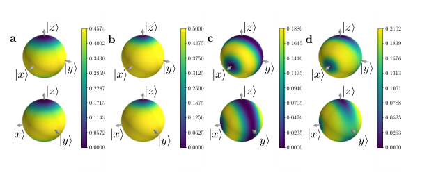
Chiral molecule. To highlight applications that will be possible on future hardware, we now turn to a simulated use of VCH to observe the quantum-to-classical transition for a chiral molecule Trost and Hornberger 2009; Coles et al. 2012. The chiral molecule has been modeled as a two level system where the right $|R\rangle$ and left $|L\rangle$ chirality states are described as $|R\rangle/|L\rangle=|+\rangle/|-\rangle=\frac{1}{\sqrt{2}}\left(|0\rangle\pm|1\rangle\right)$ Coles et al. 2012. A chiral molecule in isolation would tunnel between $|R\rangle$ and $|L\rangle$, but we consider the molecule to be in a gas, where collisions with other molecules convey information about the molecule’s chirality to its environment. This information transfer is modeled by a rotation by angle $\theta_{x}$ about the $x$ axis of an environment qubit, controlled on the system’s chirality, and for simplicity we suppose such collisions are evenly spaced at five points in time. (See Appendix E for further details.) We then consider simple families of stationary histories Coles et al. 2012, where the projector set corresponds to the same basis at all five times (just after a collision occurs). Letting $\theta_{z}$ be the precession angle due to tunneling in the time between collisions, we can then explore the competition between decoherence and tunneling. Figure 4 shows our results for this model. Notably we observe the transition from a quantum regime, where the chirality is not consistent, to a classical regime, where the chirality is both consistent and stable over time.

Figure 5 shows the circuits for computing the full trace cost (partial trace cost) from two copies of $\sigma^{\rm{A}}$ ($\sigma^{\rm{SA}}$). Note that both costs can be written as a difference of purities:

The ${\rm Tr}((\sigma^{\rm{A}})^{2})$ and ${\rm Tr}((\sigma^{\rm{SA}})^{2})$ terms are computed via the Swap Test, with a depth-two circuit and classical post-processing that scales linearly in the number of qubits Garcia-Escartin and Chamorro-Posada 2013; Cincio et al. 2018. A similar but even simpler circuit, called the Diagonalized Inner Product (DIP) Test LaRose et al. 2019, calculates the ${\rm Tr}(\mathcal{Z}^{\rm{A}}(\sigma^{\rm{A}})^{2})$ term with a depth one circuit and no post-processing. Finally, the ${\rm Tr}(\mathcal{Z}^{\rm{A}}(\sigma^{\rm{SA}})^{2})$ term is evaluated with the Partial-DIP (PDIP) Test LaRose et al. 2019, a depth-two circuit that is a hybridization of the Swap Test and the DIP Test.

One does not know a priori how many histories will be characterized in the probability readout step (Fig. 2c). Due to statistical noise, the probability of histories with greater probability will be determined with greater relative precision than those with lesser probability. Hence, it is reasonable to set a precision (or statistical noise) threshold, $\epsilon$. Let $N_{\text{readout}}$ be the number of repetitions of the probability readout circuit. Then, histories $\mathcal{Y}^{\boldsymbol{\alpha}}$ whose bitstring $\boldsymbol{\alpha}$ occurs with frequency $f_{\boldsymbol{\alpha}}<\sqrt{N_{\text{readout}}}/\epsilon_{\max}$ should be ignored, since their probabilities $p(\boldsymbol{\alpha})=f_{\boldsymbol{\alpha}}/N_{\text{readout}}$ were not characterized with the desired precision. We separate $\mathcal{F}$ into the set $\mathcal{F}_{c}$ of histories whose probabilities are above the precision threshold (which we previously referred to loosely as the most likely histories), and the set of all other histories in $\mathcal{F}$:

Computational complexity can be hidden in the value of $N_{\text{readout}}$ needed to obtain a desired precision for the probabilities of histories of interest. This issue is closely connected to the entropy of the set $\{\mathcal{D}(\boldsymbol{\alpha},\boldsymbol{\alpha})\}$, or equivalently, the entropy of the quantum state $\mathcal{Z}^{\rm{A}}(\sigma^{\rm{A}})$. When $\mathcal{Z}^{\rm{A}}(\sigma^{\rm{A}})$ is high entropy, an exponentially large number of histories may have non-zero probability, and hence $N_{\text{readout}}$ would need to grow exponentially. VCH is therefore better suited to applications where there is a small subset of the histories that are far more probable than the rest. In the parameter optimization loop, one can select for families with this property by penalizing families for which $\mathcal{Z}^{\rm{A}}(\sigma^{\rm{A}})$ has high entropy. Specifically, by noting that $P:={\rm Tr}(\mathcal{Z}^{\rm{A}}(\sigma^{\rm{A}})^{2})$ can be efficiently computed via the circuit in Fig. 5a, one can modify the costs functions in Eq. (9) and Eq. (10) to be $\tilde{C}=C/P$ and $\tilde{C}_{\rm{pt}}=C_{\rm{pt}}/P$.

We remark that classicality is intimately connected to predictability, with the emergence of classicality linked to the so-called predictability sieve Zurek 1993; Dalvit et al. 2005. Since the CH formalism is typically used to find classical families, this implies predictable families (i.e., families with low entropy or high purity $P$) are arguably of the most interest. Hence, our modified cost function $\tilde{C}$ also serves to select those consistent families with histories that are the most predictable, and therefore the most classical.

Here we discuss how VCH outputs an upper bound on the consistency parameter $\epsilon$. Let us first relate the cost $C$ to $\epsilon$. For any pair of histories $\mathcal{Y}^{\boldsymbol{\alpha}}$ and $\mathcal{Y}^{\boldsymbol{\alpha^{\prime}}}$ in $\mathcal{F}$,

which follows from Eq. (9) and the fact that $|\mathcal{D}(\boldsymbol{\alpha},\boldsymbol{\alpha}^{\prime})|=|\mathcal{D}(\boldsymbol{\alpha}^{\prime},\boldsymbol{\alpha})|$. Let us define

Then it follows from Eq. (14) that

which corresponds to the approximate consistency condition from Eq. (6). Hence, probablity sum rules for these two histories are satisfied within error $\epsilon_{\boldsymbol{\alpha},\boldsymbol{\alpha}^{\prime}}$, which can be calculated from Eq. (15) for histories in $\mathcal{F}_{c}$ since the probabilites are known for these histories.

Next, consider histories in $\overline{\mathcal{F}_{c}}$. As we do not have enough information to differentiate these histories, we advocate combining the elements of $\overline{\mathcal{F}_{c}}$ into a single coarse-grained history $\mathcal{Y}^{\boldsymbol{\gamma}}$.

Let $\mathcal{Y}^{\boldsymbol{\beta}}$ be the least likely history in $\mathcal{F}_{c}$. Then defining $\delta^{2}=\mathcal{D}(\boldsymbol{\gamma},\boldsymbol{\gamma})/\mathcal{D}(\boldsymbol{\beta},\boldsymbol{\beta})$, we can make use of the positive semi-definite property of $\sigma^{\rm{A}}$ to write:

Since $\mathcal{Y}^{\boldsymbol{\beta}}$ is the least likely history in $\mathcal{F}_{c}$, this expression then lets us bound the error on the probability sum rule (giving a weaker approximate consistency condition Dowker and Halliwell 1992) between $\mathcal{Y}^{\boldsymbol{\gamma}}$ and any $\mathcal{Y}^{\boldsymbol{\alpha}}\in\mathcal{F}_{c}$ as:

It is then possible to characterize the approximate consistency of the histories of $\mathcal{F}$ pairwise with $\epsilon_{\boldsymbol{\alpha},\boldsymbol{\alpha}^{\prime}}$ and $\delta$. Alternatively, to give an upper bound on the overall consistency $\epsilon$, we take the greatest of these pairwise bounds:

For those applications where we are working with the partial trace consistency, the notion of approximate consistency is somewhat more obscured. In order to generate probabilities and bound $\epsilon$, we therefore recommend evaluating the full trace cost function at the minimum found with the partial trace cost. This approach is helpful since any partial trace consistent family will also be full trace consistent and the partial trace consistency does not directly allow one to discuss probabilities in the same way. Taking this approach allows us to then directly utilize the approximate consistency framework above.

References

- Wheeler and Zurek (2016) J. A. Wheeler and W. H. Zurek, eds., Quantum Theory and Measurement (Princeton Series in Physics) (Princeton University Press, 2016).
- Auletta (2000) G. Auletta, Foundations and Interpretation of Quantum Mechanics (World Scientific, 2000).
- Joos and Zeh (1985) E. Joos and H. D. Zeh, “The emergence of classical properties through interaction with the environment,” Zeitschrift für Physik B Condensed Matter 59, 223–243 (1985).
- Zurek (2003) W. H. Zurek, “Decoherence, einselection, and the quantum origins of the classical,” Rev. Mod. Phys. 75, 715–775 (2003).
- Schlosshauer (2007) M. A. Schlosshauer, Decoherence: and the quantum-to-classical transition (Springer Science & Business Media, 2007).
- Griffiths (1984) R. B. Griffiths, “Consistent histories and the interpretation of quantum mechanics,” Journal of Statistical Physics 36, 219–272 (1984).
- Omnès (1988) R. Omnès, “Logical reformulation of quantum mechanics. I. foundations,” Journal of Statistical Physics 53, 893–932 (1988).
- Gell-Mann and Hartle (1989) M. Gell-Mann and J. B. Hartle, “Quantum Mechanics in the Light of Quantum Cosmology,” in Proceedings of the 3rd International Symposium Foundations of Quantum Mechanics in the Light of New Technology (1989).
- Hartle and Hertog (2017) J. Hartle and T. Hertog, “One bubble to rule them all,” Phys. Rev. D 95, 123502 (2017).
- Lloyd (2016) S. Lloyd, “Decoherent histories approach to the cosmological measure problem,” Preprint at https://arxiv.org/abs/1608.05672 (2016).
- Brun (1997) T. A. Brun, “Quantum jumps as decoherent histories,” Phys. Rev. Lett. 78, 1833–1837 (1997).
- Halliwell and Yearsley (2009a) J. J. Halliwell and J. M. Yearsley, “Quantum arrival time formula from decoherent histories,” Physics Letters A 374, 154 – 157 (2009a).
- Halliwell and Yearsley (2009b) J. J. Halliwell and J. M. Yearsley, “Arrival times, complex potentials, and decoherent histories,” Phys. Rev. A 79, 062101 (2009b).
- Anastopoulos and Savvidou (2019) C. Anastopoulos and N. Savvidou, “Time of arrival and localization of relativistic particles,” Journal of Mathematical Physics 60, 032301 (2019).
- Brun (1993) T. A. Brun, “Quasiclassical equations of motion for nonlinear brownian systems,” Phys. Rev. D 47, 3383–3393 (1993).
- Pohle (1995) H.-J. Pohle, “How to calculate decoherence matrices numerically,” Physica A: Statistical Mechanics and its Applications 213, 435 – 449 (1995).
- Schmidtke and Gemmer (2016) D. Schmidtke and J. Gemmer, “Numerical evidence for approximate consistency and markovianity of some quantum histories in a class of finite closed spin systems,” Phys. Rev. E 93, 012125 (2016).
- Preskill (2018) J. Preskill, “Quantum Computing in the NISQ era and beyond,” Quantum 2, 79 (2018).
- Peruzzo et al. (2014) A. Peruzzo, J. McClean, P. Shadbolt, M.-H. Yung, X.-Q. Zhou, P. J. Love, A. Aspuru-Guzik, and J. L. O’Brien, “A variational eigenvalue solver on a photonic quantum processor,” Nature Communications 5, 4213 (2014).
- Anschuetz et al. (2018) E. R. Anschuetz, J. P. Olson, A. Aspuru-Guzik, and Y. Cao, “Variational quantum factoring,” Preprint at https://arxiv.org/abs/1808.08927 (2018).
- Farhi et al. (2014) E. Farhi, J. Goldstone, and S. Gutmann, “A quantum approximate optimization algorithm,” Preprint at https://arxiv.org/abs/1411.4028 (2014).
- Romero et al. (2017) J. Romero, J. P. Olson, and A. Aspuru-Guzik, “Quantum autoencoders for efficient compression of quantum data,” Quantum Science and Technology 2, 045001 (2017).
- Li and Benjamin (2017) Y. Li and S. C. Benjamin, “Efficient variational quantum simulator incorporating active error minimization,” Physical Review X 7, 021050 (2017).
- Johnson et al. (2017) P. D. Johnson, J. Romero, J. Olson, Y. Cao, and A. Aspuru-Guzik, “QVECTOR: an algorithm for device-tailored quantum error correction,” Preprint at https://arxiv.org/abs/1711.02249 (2017).
- Khatri et al. (2019) S. Khatri, R. LaRose, A. Poremba, L. Cincio, A. T. Sornborger, and P. J. Coles, “Quantum-assisted quantum compiling,” Quantum 3, 140 (2019).
- LaRose et al. (2019) R. LaRose, A. Tikku, É. O’Neel-Judy, L. Cincio, and P. J. Coles, “Variational quantum state diagonalization,” npj Quantum Information 5, 57 (2019).
- Griffiths (2001) R. B. Griffiths, Consistent Quantum Theory (Cambridge University Press, 2001).
- Halliwell (1995) J. J. Halliwell, “A review of the decoherent histories approach to quantum mechanics,” Annals of the New York Academy of Sciences 755, 726–740 (1995).
- Hohenberg (2010) P. C. Hohenberg, “Colloquium: An introduction to consistent quantum theory,” Rev. Mod. Phys. 82, 2835–2844 (2010).
- Dowker and Halliwell (1992) H. F. Dowker and J. J. Halliwell, “Quantum mechanics of history: The decoherence functional in quantum mechanics,” Phys. Rev. D 46, 1580–1609 (1992).
- Riedel et al. (2016) C. J. Riedel, W. H. Zurek, and M. Zwolak, “Objective past of a quantum universe: Redundant records of consistent histories,” Phys. Rev. A 93, 032126 (2016).
- Finkelstein (1993) J. Finkelstein, “Definition of decoherence,” Phys. Rev. D 47, 5430–5433 (1993).
- McClean et al. (2016) J. R. McClean, J. Romero, R. Babbush, and A. Aspuru-Guzik, “The theory of variational hybrid quantum-classical algorithms,” New Journal of Physics 18, 023023 (2016).
- Berry et al. (2015) D. W. Berry, A. M. Childs, R. Cleve, R. Kothari, and R. D. Somma, “Simulating hamiltonian dynamics with a truncated taylor series,” Phys. Rev. Lett. 114, 090502 (2015).
- IBM (2018) “IBM Q 16 Rueschlikon backend specification,” https://github.com/Qiskit/qiskit-backend-information/tree/master/backends/rueschlikon/V1 (2018).
- Trost and Hornberger (2009) J. Trost and K. Hornberger, “Hund’s paradox and the collisional stabilization of chiral molecules,” Phys. Rev. Lett. 103, 023202 (2009).
- Coles et al. (2012) P. J. Coles, V. Gheorghiu, and R. B. Griffiths, “Consistent histories for tunneling molecules subject to collisional decoherence,” Phys. Rev. A 86, 042111 (2012).
- Paz and Zurek (1993) J. P. Paz and W. H. Zurek, “Environment-induced decoherence, classicality, and consistency of quantum histories,” Phys. Rev. D 48, 2728–2738 (1993).
- Zurek et al. (2005) W. H. Zurek, U. Dorner, and P. Zoller, “Dynamics of a Quantum Phase Transition,” Phys. Rev. Lett. 95, 105701 (2005).
- Allegra et al. (2016) M. Allegra, P. Giorda, and S. Lloyd, “Global coherence of quantum evolutions based on decoherent histories: Theory and application to photosynthetic quantum energy transport,” Phys. Rev. A 93, 042312 (2016).
- Liu et al. (2001) H. Liu, M. Elstner, E. Kaxiras, T. Frauenheim, J. Hermans, and W. Yang, “Quantum mechanics simulation of protein dynamics on long timescale,” Proteins 44, 484–489 (2001).
- Poulin (2002) D. Poulin, “Classicality of quantum information processing,” Phys. Rev. A 65, 042319 (2002).
- Bloembergen (1949) N. Bloembergen, “On the interaction of nuclear spins in a crystalline lattice,” Physica 15, 386 – 426 (1949).
- Lowe and Gade (1967) I. J. Lowe and S. Gade, “Density-matrix derivation of the spin-diffusion equation,” Phys. Rev. 156, 817–825 (1967).
- Dumez (2011) J.-N. Dumez, Many body dynamics in nuclear spin diffusion, Theses, Ecole normale supérieure de lyon - ENS LYON (2011).
- Adachi et al. (2012) S. Adachi, R. Kaji, S. Furukawa, Y. Yokoyama, and S. Muto, “Nuclear spin depolarization via slow spin diffusion in single InAlAs quantum dots observed by using erase-pump-probe technique,” Journal of Applied Physics 111, 103531 (2012).
- Englander and Mayne (2017) S. W. Englander and L. Mayne, “The case for defined protein folding pathways,” Proceedings of the National Academy of Sciences 114, 8253–8258 (2017).
- Eaton and Wolynes (2017) W. A. Eaton and P. G. Wolynes, “Theory, simulations, and experiments show that proteins fold by multiple pathways,” Proceedings of the National Academy of Sciences 114, E9759–E9760 (2017).
- Garcia-Escartin and Chamorro-Posada (2013) J. C. Garcia-Escartin and P. Chamorro-Posada, “Swap test and Hong-Ou-Mandel effect are equivalent,” Physical Review A 87, 052330 (2013).
- Cincio et al. (2018) L. Cincio, Y. Subaşı, A. T. Sornborger, and P. J. Coles, “Learning the quantum algorithm for state overlap,” New Journal of Physics 20, 113022 (2018).
- Zurek (1993) W. H. Zurek, “Preferred States, Predictability, Classicality and the Environment-Induced Decoherence,” Progress of Theoretical Physics 89, 281–312 (1993).
- Dalvit et al. (2005) D. A. R. Dalvit, J. Dziarmaga, and W. H. Zurek, “Predictability sieve, pointer states, and the classicality of quantum trajectories,” Phys. Rev. A 72, 062101 (2005).
- Gell-Mann and Hartle (1993) M. Gell-Mann and J. B. Hartle, “Classical equations for quantum systems,” Phys. Rev. D 47, 3345–3382 (1993).
- Zhang et al. (1992) S. Zhang, B. H. Meier, and R. R. Ernst, “Polarization echoes in nmr,” Phys. Rev. Lett. 69, 2149–2151 (1992).
- Torgny et al. (1995) K. Torgny, H. Michael, N. D. Kurur, and M. H. Levitt, “Rotational resonance echoes in the nuclear magnetic resonance of spinning solids,” Chemical Physics Letters 247, 534 – 540 (1995).
- Tomaselli et al. (1996) M. Tomaselli, S. Hediger, D. Suter, and R. R. Ernst, “Nuclear magnetic resonance polarization and coherence echoes in static and rotating solids,” The Journal of Chemical Physics 105, 10672–10681 (1996).
- Piana et al. (2013) S. Piana, K. Lindorff-Larsen, and D. E. Shaw, “Atomic-level description of ubiquitin folding,” Proceedings of the National Academy of Sciences 110, 5915–5920 (2013).
Supplementary Material for