A generalised framework for non-classicality of states II:
Emergence of non locality and entanglement

Soumik Adhikary Email: soumikadhikary@physics.iitd.ac.in Affiliation: Department of Physics, Indian Institute of Technology Delhi, New Delhi-110016, India. Sooryansh Asthana Email: sooryansh.asthana@physics.iitd.ac.in Affiliation: Department of Physics, Indian Institute of Technology Delhi, New Delhi-110016, India. V. Ravishankar Email: vravi@physics.iitd.ac.in Affiliation: Department of Physics, Indian Institute of Technology Delhi, New Delhi-110016, India.

August 11, 2026

Abstract

A unified formalism was developed in Adhikary et al. 2019, for describing non classicality of states by introducing pseudo projection operators in which both quantum logic and quantum probability are naturally embedded. In this paper we show, as the first practical application, how non-locality and entanglement emerge as two such important manifestations. It provides a perspective complementary to (i) the understanding of them that we have currently Bell 1964; Clauser et al. 1969; Werner 1989, and (ii) to the algebraic approaches employed. The work also makes it possible to obtain, in a systematic manner, an infinite number of conditions for non-classicality, for future applications.

pacs

03.65.Ca, 03.65.Ud, 03.67.Mn, 03.67.-a

I Introduction

The idea of non-classicality of states is a unique feature of quantum mechanics that distinguishes it from both classical physics and classical probability Dirac 1942; Bartlett 1945; Accardi 1981; Feynman 2012. Thus, it is pivotal to applications in quantum information and computation Bennett and Brassard 1984; Shor 1997; Bennett et al. 1993; Deutsch and Josza 1992. For this reason, depending on the exigencies of situation, many standards of non classicality, such as non-locality, entanglement, steering, and discord have been proposed Bell 1964; Clauser et al. 1969; Peres 1996; Wiseman et al. 2007; Ollivier and Zurek 2001. The need of the day is a common unifying framework from which these many facets can be understood in a natural fashion. It would also allow setting up criteria of non-classicality in a systematic fashion.

We have recently set up one such framework, hereafter denoted by I Adhikary et al. 2019, in which we introduce operators which we designate as pseudo projections. Non-classicality of states is captured by the associated pseudo probabilities which admit negative values. The formalism, which we recapitulate briefly in section II, is entirely free of ad-hoc constructions, and it has been shown that quantum logic and quantum probability are inherent to the formalism. These were illustrated mainly with the example of two level systems.

As a direct continuation of I, this paper shows how two important standards of non-classicality – non locality and entanglement, emerge as direct manifestations of quantum probability and quantum logic. We show, with a judicious choice of classical logical propositions and/or combinations of pseudo probabilities in a given scheme, the emergence of Bell-CHSH non-locality in any dimension, and quantitative signatures for entanglement in $2\times 2$ dimensional spaces. Thereby, this new demonstration also brings out yet another essential aspect of these important criteria.

II Preliminaries

We begin with a quick recapitulation of pseudo projections and pseudo probabilities which were introduced in I.

II.1 Indicator function and their quantum representatives

We start with classical observables $A,B,\cdots$ defined over a phase space $\Phi$ ¹¹ 1 More generally, it could be any sample space. Let $S^{A}_{i}\subset\Phi$ be the support for the outcome $A=a_{i}$ . Similarly, let $S^{B}_{j}\subset\Phi$ be the support for the outcome $B=b_{j}$ . If a system is in a state $f$ , the respective probabilities for the outcomes will be given by the overlap of $f$ with the corresponding indicator functions $I_{S^{A}_{i}}$ and $I_{S^{B}_{j}}$ . The indicator functions are boolean observables, taking the value +1 within the support and zero outside. For a given observable, the supports $S_{i}$ are mutually disjoint, and partition $\Phi$ : $S_{i}\bigcap S_{j}=\emptyset;\penalty\ \penalty\ \bigcup\limits_{i}S_{i}=\Phi$ .

Consider the transition to the quantum domain. The phase space maps to a Hilbert space $H$ , and a classical state – to a density operator $\rho$ . An observable $A$ maps to a self adjoint operator denoted, again, by $A$ and which admits the spectral decomposition, $A=\sum_{i}a_{i}\pi^{A}_{i}$ ; the eigen projections $\pi^{A}_{i}$ partition $H$ into a disjoint union of subspaces, ${\cal H}=\bigcup\limits_{i}\oplus{\cal H}^{A}_{i}$ . Finally, the probability for the outcome $A=a_{i}$ is given by the overlap $p^{A}_{i}=Tr(\rho\pi^{A}_{i})$ . All other outcomes are disallowed.

Two important mappings that follow are of particular relevance: $I_{S^{A}_{i}}\rightarrow\pi_{i};\penalty\ \penalty\ S^{A}_{i}\rightarrow H_{i}$ . However, not all of these projections are the eigen projections of the operator. In fact, very many indicator functions would map to the trivial projection $\pi=0$ (unless the spectrum is continuous), in which case, the corresponding supports $S_{i}\rightarrow\emptyset$ , the null space.

In short, the indicator functions either map to eigen projections, or their sums thereof, or to the trivial null operator. Similarly the supports map to either the eigen subspaces or their direct sums thereof, or to the null set $\emptyset$ . There is no other possibility.

II.2 Pseudoprojections for two observables

The situation changes when joint outcomes of observables is considered. Classically, the probability for a joint outcome $A=a_{i},B=b_{j}$ is equally easy to determine. One evaluates the overlap of the classical state $f$ with the indicator function defined over the intersection of the corresponding supports $S_{i}\cap S_{j}$ (we suppress the observable index henceforth, unless necessary).

The quintessential feature of quantum probability is that $I_{S_{i}\bigcap S_{j}}$ does not map to a projection, unless the projections for the two outcomes commute. Assignment of a joint probability is thus disallowed in most cases. It does not forbid, however, the very question as to what the quantum representative of $I_{S_{i}\bigcap S_{j}}$ is. Recall that, classically, $I_{S_{i}\bigcap S_{j}}$ is itself a Boolean observable. The answer to this question holds the key to formulate and understand the non-classical features of quantum probability.

The answer may be inferred from rules of quantum mechanics. The quantum representative is just the symmetrised product of the projection operators:

I_{S_{i}\bigcap S_{j}}\equiv I_{S_{i}}I_{S_{j}}\rightarrow{\bf\Pi}_{ij}=\frac{1}{2}(\pi_{i}\pi_{j}+\pi_{j}\pi_{i}).

(1)

The quantum representative ${\bf\Pi}_{ij}$ is hermitian, but not a projection, unless $[\pi_{i},\pi_{j}]=0$ . This is but the simplest example of operators that we shall designate as pseudo projections. ${\bf\Pi}_{ij}$ possesses two essential properties: (i) As proved in I, it has at least one negative eigenvalue. (ii) The set, ${\cal S}^{2}=\Big\{{\bf\Pi}_{ij}\Big\}$ , of all pseudo projections corresponding to all possible joint outcomes of two observables, $A,B$ forms an over-complete set of operators and yields a resolution of identity, as given by

	$\displaystyle\sum_{i}\sum_{j}{{\bf\Pi}_{ij}}$	$\displaystyle=$	$\displaystyle\sum_{i}\pi_{i}=\mathbb{1}$
	$\displaystyle\sum_{j}\sum_{i}{{\bf\Pi}_{ij}}$	$\displaystyle=$	$\displaystyle\sum_{j}\pi_{j}=\mathbb{1}$		(2)

The proof is a direct consequence of completeness of eigen projections of any observable.

II.3 Pseudoprojection operators for multiple observables

More generally, quantum representatives of indicator functions representing joint outcomes of $N$ observables will be called pseudo projections. We are interested in the stuation when they are mutually incpmpatible. When $N\geq 3$ , thet are not unique. Consider, thus, a conjunction of $N$ events $\Big\{A^{k}=a^{k}_{i_{k}};\penalty\ \penalty\ k=1,2,\cdots,N\Big\}$ , where the index $k$ labels the observable. If we were to denote the product of the corresponding projection operators in some order – collectively denoted by the ordered set { $\alpha$ } — by ${\cal A}^{N}_{\{\alpha\}}$ , then the hermitised sum

{\bf\Pi}^{N}_{\{\alpha\}}=\frac{1}{2}({\cal A}^{N}_{\{\alpha\}}+{\cal A}^{N{\dagger}}_{\{\alpha\}})

(3)

serves as a valid quantum representative of the classical indicator function, i.e., it is a pseudo projection. We call this a unit pseudo projection.

There are $\frac{N!}{2}$ such unit pseudo-projections, depending on the order in which the projection operators are arranged. The representative pseudo projection can be chosen to be any element in the convex span of these unit pseudo projections:

\sum_{\{\alpha\}}\lambda_{\{\alpha\}}{\bf\Pi}^{N}_{\{\alpha\}}\rightarrow{\bf\Pi}^{N}(\{\lambda_{\{\alpha\}}\})

(4)

i.e.,

0\leq\lambda_{\{\alpha\}}\leq 1;\penalty\ \sum_{\{\alpha\}}\lambda_{\{\alpha\}}=1.

(5)

In general, each point in the manifold yields an inequivalent quantum representative of the underlying indicator function. The manifold would collapse to a point if all the projections were to commute.

The richness afforded by this non uniqueness, for exploring fully all the aspects of quantum probability, deserves a separate study. For the present purposes, in this paper, we employ, as in I, only the completely symmetric combination, and denote it, generically, by ${\bf\Pi}^{N}$ .

Pseudo projections with $N$ observables also satisfy the following over completeness relation: Let ${\cal S}^{N}_{\{\alpha\}}$ be the set of all pseudo projections corresponding to all possible outcomes of the $N$ observables at hand. Let $\{\alpha\}=\{\beta,j\}$ where $j$ refers to the outcomes of the observable labelled $A^{k}$ and $\beta$ collectively denote the rest. Then,

\sum_{j}{\bf\Pi}^{N}_{\{\beta,j\}}={\bf\Pi}^{N-1}_{\{\beta\}}.

(6)

as in ${\cal S}^{2}$ , it is a direct consequence of the completeness of eigen projections of observables. It may also be shown that unit pseudo-projections also possess negative eigenvalues.

III Pseudo Probability and Non Classicality

As pointed out in I, pseudo projections generate pseudo probabilities. Let a system be in a state $\rho$ . We then define the pseudo probability associated with a pseudo projection to be

\mathcal{P}^{N}=Tr\Big\{\rho{\bf\Pi}^{N}\Big\}

(7)

Since ${\bf\Pi}^{N}$ can admit negative eigenvalues, the corresponding pseudo probability can also be negative. We shall designate the set of all pseudo probabilities generated by a set ${\cal S}^{N}$ – a pseudo probability scheme. By virtue of relations in Eqs.(II.2) and (6), it follows that pseudo probabilities in any scheme add up to one. As a corollary of Eq.(6), pseudo probability schemes for subsets of observables are just the marginals of the parent scheme.

Pseudo-probability schemes allow us to define non-classicality in a very broad sense. A state $\rho$ is deemed to be non-classical with respect to a set of observables $\{A_{i}\}$ , even if a single entry in the corresponding pseudo probability scheme is negative. Conversely, a state would be called classical with respect to the same set of observables iff all the entries in the scheme are non-negative.

As a corollary, sums of pseudo probabilities can also assume value ouside [0, 1], and can serve as signatures of non classicality.

III.0.1 Other logical operations

It is convenient to set up the quantum representatives of indicator functions representing disjunction and negation, directly from the appropriate suitable pseudo probability schemes, i.e., by employing standard probability rules. For example, the operator that corresponds to the disjunction, $A=a_{i}$ OR $B=b_{j}$ , can be obtained from the joint pseudo probability scheme for observables $A,B$ , as follows:

	$\displaystyle{\bf R}_{a_{i}b_{j}}^{AB}$	$\displaystyle=\sum_{l}{\bf\Pi}_{a_{i}b_{l}}^{AB}+\sum_{l}{\bf\Pi}_{a_{l}b_{j}}^{AB}-{\bf\Pi}_{a_{i}b_{j}}^{AB}$
		$\displaystyle={\pi}_{a_{i}}^{A}+{\pi}_{b_{j}}^{B}-{\bf\Pi}_{a_{i}b_{j}}^{AB}$		(8)

Similarly, the quantum representative of the negation of an event is obtained by subtracting its representative pseudo projection from identity.

Just as in conjunction (joint events), and even more so, the expression for OR given above is prescriptive, and not completely inferred. This is not a drawback since other prescriptions reflect, again, the inherent ambiguity in the construction of quantum analogs of classical entities. A further discussion of this richness is, at this stage, an unnecessary digression.

As in many other fortunate situations, it is not always necessary to have a full knowledge of the scheme to derive some of the important tests for non-classicality. It is most certainly true of Bell CHSH non-locaility, as we show below. And again, many good tests for entanglement can be devised with a much smaller set of pseudoprobabilities.

We devote the rest of the paper to demonstrate just this: how non-locality and entanglement can be understood as natural manifestations of quantum logic and quantum probability, both of which are captured by pseudo probabilities. The propositions involve pseudoprojections and quantum representatives of other logical operations involving disjunction and negation . These results go way beyond the ones obtained in I for single systems.

IV Notations and Pictorial Representations

First, we establish some notations for the sake of compactness. All observables, considered henceforth, are dichotomic, with eigenvalues $\pm 1$ . Thus, the two outcomes are negations of each other. The proposition $\mathcal{L}(A=+1)$ is denoted by $\mathcal{L}(A)$ , and its negation, $\mathcal{L}(A=-1)$ , by $\mathcal{L}(\overline{A})$ . Conjunctions are written as simple juxtapositions, by omitting the sign $\wedge$ . However, the OR operation (disjunction) will be explicitly denoted by the standard symbol $\vee$ . We agree to separate observables belonging to different subsystems by a semicolon. The following example illustrates the notations.

\mathcal{L}\{A_{1}=+1\}\wedge\mathcal{L}\{B_{1}=-1\}\wedge\mathcal{L}\{B_{2}=+1\}\equiv\mathcal{L}\{A_{1};\overline{B}_{1}B_{2}\}

(9)

Here, the observables $A_{1}$ and $B_{1,2}$ belong to the first and the second subsystems respectively. The pseudoprobability corresponding to $A=+1$ is denoted by $\mathcal{P}(A)$ , and the one for its negation, $A=-1$ , by $\mathcal{P}(\overline{A})$ . For example, the pseudoprobability corresponding to the proposition in Eq.( 9) will be denoted by $\mathcal{P}\{A_{1};\overline{B}_{1}B_{2}\}$ .

We also introduce a pictorial representation alongside the algebraic expressions for the logical propositions since the latter can be lengthy, and not easily tractable. This is illustrated in Fig.(1) where, the observables in the first and second subsystems are indicated by blue and green respectively. The outputs $\pm 1$ for an observable are indicated by a red button in the appropriate slot. Entries in a given row refer to conjunction (AND) and different rows are related by disjunction (OR), as indicated by the double bond.

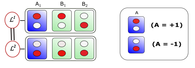
Refer to caption — Figure 1: Pictorial representation of the proposition $\mathcal{L}^{1}\{A_{1};B_{1}\overline{B}_{2}\}\vee\mathcal{L}^{2}\{\overline{A}_{1};\overline{B}_{1}\overline{B}_{2}\}$ . Inset: The pictorial representation of the outputs $\pm 1$ of an observable.

V Non-locality and Entanglement from logical propositions

This section, together with the next, contains the main results of this paper. Our approach here is two pronged. In the first, we demonstrate the break down of elementary logical propositions — more precisely, of the associated probability, for non locality and entanglement. In the former case, we show the emergence of the Bell-CHSH inequality for all $M\times N$ level systems. In the latter case, a set of witnesses are derived for $2\times 2$ level systems.

A word or two on how the propositions are constructed. We employ two guide lines. The propositions probe only the correlation space of the state by masking the nonclassicality coming from the subsystems. We further ensure that at least two or more noncommuting bases are involved which is essential to bring out the difference between separable and entangled states.

V.1 Non-locality

Consider an $M\times N$ level system, and pairs of dichotomic observables, $A_{1,2}$ and $B_{1,2}$ , belonging to respective subsystems. The underlying scheme $\mathcal{P}(A_{1}A_{2};B_{1}B_{2})$ consists of 16 entries. Of interest is the simplest of the nontrivial propositions involving incompatible observables, which are shown in Fig. (2) — both algebraically and pictorially.

The supports $S_{i}$ for the classical outcomes for their corresponding conjunctions $\mathcal{L}^{i}$ in Fig.(2) are mutually disjoint. Accordingly, its indicator function $I_{S}$ for the proposition in Fig.(2) is given by the sum of the corresponding indicator functions,

{I}_{S}=\sum_{i=1}^{4}{I}_{S_{i}}.

(10)

The quantum representative of $I_{S}$ is the corresponding sum, ${\bf{\Pi}}_{N}=\sum_{i}{\bf\Pi}_{i}$ of the pseudo projections representing each conjunction. Note that none of the pseudo-projections in the summand is a projection. A state $\rho$ would be classical with respect to this proposition if the corresponding pseudo-probability respects the bounds

0\leq Tr\Big[\rho{\bf\Pi}_{N}\Big]\leq 1

(11)

The identity, $\pi^{A}_{\pm 1}=\frac{1}{2}(1\pm A)$ , immediately leads to the classic Bell-CHSH inequality

\Big|\Big<A_{1}B_{1}+A_{1}B_{2}+A_{2}B_{1}-A_{2}B_{2}\Big>_{\rho}\Big|\leq 2

(12)

Comparison with other derivations: This derivation essentially identifies the inadmissibility of standard Boolean rules to operations on a set of logical propositions. Thereby, it throws further light on the violation of the corresponding rule of classical probability in the form expressed in Clauser et al. 1969. Truly, violation of Bell - CHSH inequality is autonomous of the kinematics of inertial frames. Hence, it stands in stark contrast with the very first derivation which employed space like separations. This observation does, by no means, diminish the deep physical and philosophical consequences that follow from combining non-locality with special relativity. The derivation also shows that jointly measurable observables cannot lead to the violation of the Bell-CHSH inequality Fine 1982a; Fine 1982b; Khalfin and Tsirelson 1985; Wolf et al. 2009. It will be seen that this last conclusion continues to hold true for entanglement also.

For future comparison, we recast Eq. (12) for the two-qubit case in terms of correlations, for the special geometry $Tr(A_{1}A_{2})=Tr(B_{1}B_{2})=0$ . We employ the forms $A_{1,2}=\vec{\sigma}\cdot\hat{a}_{1,2}$ and $B_{1,2}=\vec{\Sigma}\cdot\hat{b}_{1,2}$ in terms of the Pauli bases in the respective subspaces. Writing the normalised sum of vectors as $\hat{b}=\frac{1}{\sqrt{2}}(\hat{b}_{1}+\hat{b}_{2})$ and $\hat{b}^{\prime}=\frac{1}{\sqrt{2}}(\hat{b}_{1}-\hat{b}_{2})$ , we obtain the following inequality for nonlocality,

\Big|\Big<\vec{\sigma}\cdot\hat{a}_{1}\vec{\Sigma}\cdot\hat{b}+\vec{\sigma}\cdot\hat{a}_{2}\vec{\Sigma}\cdot\hat{b}^{\prime}\Big>\Big|_{\rho}>\sqrt{2}.

(13)

V.2 Entanglement

Though all non-local states are entangled, the converse statement is not necessarily trueWerner 1989, suggesting that entanglement admits further refinements. Further, settling whether a state is entangled or not is considered to be a hard problem, which has led to several more modest approaches such as majorisation relations, conditions based on correlation tensors and studies involving concurrence Nielsen and Kempe 2001; Mintert et al. 2004; de Vicente and Huber 2011. Rather than hunt for a single proposition that would deliver a witness which is capable of detecting all entangled states, we take up two-qubit systems, and systematically construct two inequivalent logical propositions of increasing complexity and three combinations of appropriate pseudo-probabilities, and show that each of them yields an entanglement witness, emphasising the breakdown of the validity of an underlying classical proposition.

V.2.1 Proposition 1

Let $A$ stand for the observable $\vec{\sigma}\cdot\hat{a}$ . Henceforth, we denote the observables in the first and the second subsystems respectively by Latin and Greek symbols. The respective Pauli operators will be denoted by $\sigma_{i}$ and $\Sigma_{i}$ . The first proposition has the same number of observables as in non locality, but with additional constraints. This leads to inclusion of more states in the set of entangled states.

Thus, let two doublets of observables, $\{A_{1},A_{2}\}$ and $\{\Phi_{1},\Phi_{2}\}$ belong to the first and the second qubit respectively. They further obey the orthonormality conditions $\hat{a}_{1}\cdot\hat{a}_{2}=\hat{\phi}_{1}\cdot\hat{\phi}_{2}=0$ . The proposition, which is more complex than the one for non-locality, is displayed in Fig.(3), together with the attendant pictorial representation.

As with non-locality and all other subsequent examples, a state is classical if the associated pseudo probability is non-negative. Mimicking the steps just employed, we arrive at the first sufficiency condition for entanglement, which is given by

\Big<\vec{\sigma}\cdot\hat{a}_{1}\vec{\Sigma}\cdot\hat{\phi}_{1}+\vec{\sigma}\cdot\hat{a}_{2}\vec{\Sigma}\cdot\hat{\phi}_{2}\Big>_{\rho}<-1.

(14)

The correlations in the LHS of Eq. (14) are the same as in Eq.(13). But the bound in the RHS renders more states non-classical, restating the fact that there are entangled states which are local. More importantly, it exhibits the logical distinction between local and non-local entangled states, complementing the view point emphasised in Werner 1989. This distinction raises the possibility that inclusion of more observables (classical joint observations) may lead to even better witnesses and further logical distinctions within the family of entangled states.

V.2.2 Proposition 2

We now consider two triplets each of three orthonormal observables – $\{A_{i}\},\penalty\ \{\Phi_{i}\};\penalty\ i\in\{1,2,3\}$ for the first and second qubit respectively. More explicitly, $Tr(A_{i}A_{j})=Tr(\Phi_{i}\Phi_{j})=\delta_{i,j}$ . The parent pseudo-probability scheme, $\mathcal{P}(A_{1}A_{2}A_{3};\Phi_{1}\Phi_{2}\Phi_{3})$ , would consist of $2^{6}$ entries. But for our purposes, it suffices to examine a smaller combination of disjunctions shown in Fig.(4),involving only eight pseudo probabilities.

Yet again, for the same reasons stated above, the pseudo projection for the unions is simply the sum of each pseudo projection for individual conjunctions. Violation of the non negativity requirement for the associated pseudo probability for classicality yields the following sufficiency condition for a state to be entangled:

\Big<\vec{\sigma}\cdot\hat{a}_{1}\vec{\Sigma}\cdot\hat{\phi}_{1}+\vec{\sigma}\cdot\hat{a}_{2}\vec{\Sigma}\cdot\hat{\phi}_{2}+\vec{\sigma}\cdot\hat{a}_{3}\vec{\Sigma}\cdot\hat{\phi}_{3}\Big>_{\rho}<-1

(15)

The inequality (15) is not new, and has been derived earlier by Gühne et al. Gühne et al. 2003 and Werner Werner 1989. We note that their derivation is driven by purely algebraic considerations, and that their results were stated for one specific geometry, $\hat{a}_{1}=\hat{\phi}_{1}=\hat{x};\ \ \hat{a}_{2}=\hat{\phi}_{2}=\hat{y};\ \ \hat{a}_{3}=\hat{\phi}_{3}=\hat{z}$ , in contrast to our approach which is motivated by violations of classical rules of probability associated with operations. An even more direct derivation of this inequality will be given in the next section.

VI Entanglement from direct violations of classical probability rules

We do away with the task of explicit formulation in terms of underlying logical propositions and instead, deal with the entries in the pseudo probability schemes directly.

VI.0.1 Inequality 1

First, we consider a pair of mutually orthogonal observables $A_{1}$ , $A_{2}$ for the first qubit and two triplets of orthonormal observables $\{\Phi_{1},\Phi_{2},\Phi_{3}\},\{\Theta_{1},\Theta_{2},\Theta_{3}\}$ for the second. To specify the detector geometry completely, the normalised sums of the vectors, in the respective triplets $\{\Phi_{i}\}$ and $\{\Theta_{i}\}$ , given by $\hat{\phi}=\sum_{i=1}^{3}\hat{\phi}_{i}/\sqrt{3}$ and $\hat{\theta}=\sum_{i=1}^{3}\hat{\theta}_{i}/\sqrt{3}$ , are chosen to be orthogonal: $\hat{\phi}\cdot\hat{\theta}=0$ . The number of pseudo probabilities in the scheme is $2^{8}$ and holds a wealth of information. But for our purposes, we may look at the sum of the marginals of merely four pseudo probabilities

	$\displaystyle\mathcal{S}_{1}$	$\displaystyle=$	$\displaystyle\mathcal{P}\{A_{1};\Phi_{1}\Phi_{2}\Phi_{3}\}+\mathcal{P}\{\overline{A}_{1};\overline{\Phi}_{1}\overline{\Phi}_{2}\overline{\Phi}_{3}\}$		(16)
		$\displaystyle+$	$\displaystyle\mathcal{P}\{A_{2};\Theta_{1}\Theta_{2}\Theta_{3}\}+\mathcal{P}\{\overline{A}_{2};\overline{\Theta}_{1}\overline{\Theta}_{2}\overline{\Theta}_{3}\}.$		(16)

Classicality would force $\mathcal{S}_{1}$ to be non-negative. Its violation yields a sufficiency condition for entanglement given by

\Big<\vec{\sigma}\cdot\hat{a}_{1}\vec{\Sigma}\cdot\hat{\phi}+\vec{\sigma}\cdot\hat{a}_{2}\vec{\Sigma}\cdot\hat{\theta}\Big>_{\rho}<-\frac{2}{\sqrt{3}},

(17)

VI.0.2 Inequality 2

The next inequality may be derived by enlarging the scheme further. For the first subsystem, we consider three orthonormal sets of doublets of observables $\{A_{i}\}$ , $\{B_{i}\}$ $\{C_{i}\}$ . For the second system, we choose three orthonormal sets of triplets of observables $\{\Phi_{i}\},\{\Theta_{i}\},\{\Psi_{i}\}$ . As in the earlier cases, the detector geometry is specified by requiring that both the sets of normalised sums { $\hat{a},\hat{b},\hat{c}$ } and { $\hat{\phi},\hat{\theta},\hat{\psi}$ } be orthonormal sets. The sum of marginals of interest is

$\displaystyle\mathcal{S}_{2}$	$\displaystyle=$	$\displaystyle\mathcal{P}\{A_{1}A_{2};\Phi_{1}\Phi_{2}\Phi_{3}\}+\mathcal{P}\{\overline{A}_{1}\overline{A}_{2};\overline{\Phi}_{1}\overline{\Phi}_{2}\overline{\Phi}_{3}\}$	(18)
	$\displaystyle+$	$\displaystyle\mathcal{P}\{B_{1}B_{2};\Theta_{1}\Theta_{2}\Theta_{3}\}+\mathcal{P}\{\overline{B}_{1}\overline{B}_{2};\overline{\Theta}_{1}\overline{\Theta}_{2}\overline{\Theta}_{3}\}$
	$\displaystyle+$	$\displaystyle\mathcal{P}\{C_{1}C_{2};\Psi_{1}\Psi_{2}\Psi_{3}\}+\mathcal{P}\{\overline{C}_{1}\overline{C}_{2};\overline{\Psi}_{1}\overline{\Psi}_{2}\overline{\Psi}_{3}\}$

which leads to an independent sufficiency condition, i.e., a new witness for non-separability, which has the form

\Big<\vec{\sigma}\cdot\hat{a}\vec{\Sigma}\cdot\hat{\phi}+\vec{\sigma}\cdot\hat{b}\vec{\Sigma}\cdot\hat{\theta}+\vec{\sigma}\cdot\hat{c}\vec{\Sigma}\cdot\hat{\psi}\Big><-\sqrt{\frac{3}{2}}

(19)

VI.0.3 Inequality 3

Finally, we consider three orthonormal triplets $\{A_{i}\},\{B_{i}\},\{C_{i}\}$ for the first qubit, and similarly three orthonormal triplets of $\{\Phi_{i}\},\{\Theta_{i}\},\{\Psi_{i}\}$ for the second. As before, the normalised sums are chosen to be mutually orthogonal for each qubit. The convex sum of the marginals of pseudo probabilities, which is more involved, is displayed in Eq. (VI.0.3).

$\displaystyle\mathcal{S}_{3}$	$\displaystyle=$	$\displaystyle\mathcal{P}\{A_{1}A_{2}A_{3};\Phi_{1}\Phi_{2}\Phi_{3}\}+\mathcal{P}\{\overline{A}_{1}\overline{A}_{2}\overline{A}_{3};\overline{\Phi}_{1}\overline{\Phi}_{2}\overline{\Phi}_{3}\}$
	$\displaystyle+$	$\displaystyle\mathcal{P}\{B_{1}B_{2}B_{3};\Theta_{1}\Theta_{2}\Theta_{3}\}+\mathcal{P}\{\overline{B}_{1}\overline{B}_{2}\overline{B}_{3};\overline{\Theta}_{1}\overline{\Theta}_{2}\overline{\Theta}_{3}\}$
	$\displaystyle+$	$\displaystyle\mathcal{P}\{C_{1}C_{2}C_{3};\Psi_{1}\Psi_{2}\Psi_{3}\}+\mathcal{P}\{\overline{C}_{1}\overline{C}_{2}\overline{C}_{3};\overline{\Psi}_{1}\overline{\Psi}_{2}\overline{\Psi}_{3}\}$

The resulting inequality yields an improved sufficiency condition for entanglement, given by

\Big<\vec{\sigma}\cdot\hat{a}\vec{\Sigma}\cdot\hat{\phi}+\vec{\sigma}\cdot\hat{b}\vec{\Sigma}\cdot\hat{\theta}+\vec{\sigma}\cdot\hat{c}\vec{\Sigma}\cdot\hat{\psi}\Big><-1

This inequality is the same given in Eq. (15), thus demonstrating that employing a scheme or looking for violations of propositions are but two equivalent approaches. It is entirely a matter of convenience as to which approach is to be used.

More pertinently, this analysis shows that none of these non-classicality conditions would follow if all the entries in the underlying pseudo-probability scheme were non-negative. A seemingly similar approach involving quasi probabilities Puri 2012 does not yield witnesses since a prior knowledge of the state is assumed to determine if the state is entangled.

Just as with the distinction between non-locality and entanglement, the inequalities derived in this section induce a further refinement in characterising entanglement, depending on the set of classical rules violated by the states. We explore their interrelationship in greater detail in the next section.

VII Examples and discussion

We label the five inequalities for entanglement, 13, 17, 14, 19 and 15 as ${\bf W_{0}},{\bf W_{1}},{\bf W_{2}},{\bf W_{3}}$ and ${\bf W_{4}}$ respectively. For illustration, and further discussion, we shall begin with the special class of states, obtained by the addition of a local term to the Werner states,

\rho=\frac{1}{4}(1+\alpha\vec{\sigma}\cdot\vec{\Sigma}+\beta\sigma_{z}).

(21)

The main results are captured in Fig. (5). The region bounded by the points $A,B,C$ and $D$ , represents the space of all allowed states. The line $AC$ represents the Werner states, and the region contained between the arcs $BED$ and $BCD$ corresponds to separable states. The vertex $A$ represents the fully entangled singlet state, and the point $O$ , the completely mixed state.

The five vertical lines mark the boundaries of sets of entangled states (triangles with $A$ as their common vertex) detected by respective propositions. Of them, the first line $L_{0}$ marks the boundary between non-local and local states. The subsequent lines represent, in order, the sets encompassed by the set of four sufficiency conditions, ${\bf W_{i}}$ , in the same order. The last line, $L_{4}$ encompasses the largest region, which includes all the entangled Werner states. But it is still not exhaustive since it fails to detect entangled states in the region shaded in pink. The existence of a logical proposition that would lead to a witness that detects all the entangled state is yet to be demonstrated.

It is possible to draw several strong conclusions for more general states. Consider an arbitrary two-qubit state in the SVD basis,

\rho=\frac{1}{4}(1+\vec{P}\cdot\vec{\sigma}+\vec{Q}\cdot\vec{\Sigma}+\sum_{i=1}^{3}t_{i}\sigma_{i}\Sigma_{i}).

(22)

The witnesses, comprising entirely of correlations, are sensitive only to the singular values $t_{i}$ . Each witness, therefore detects entangled states in regions, determined by the corresponding set of inequalities imposed on the singular values. The region of the correlation space that represents a state is a tetrahedron, defined by the four inequalities Horodecki and Horodecki 1996,

$\displaystyle 1-t_{1}-t_{2}-t_{3}$	$\displaystyle\geq$	$\displaystyle 0$
$\displaystyle 1-t_{1}+t_{2}+t_{3}$	$\displaystyle\geq$	$\displaystyle 0$
$\displaystyle 1+t_{1}-t_{2}+t_{3}$	$\displaystyle\geq$	$\displaystyle 0$
$\displaystyle 1+t_{1}+t_{2}-t_{3}$	$\displaystyle\geq$	$\displaystyle 0.$	(23)

First consider the witness ${\bf W_{4}}$ . It partitions the correlation space into two parts. States that are separable and those that are entangled but evade detection by ${\bf W_{4}}$ , satisfy the conditions:

$\displaystyle 1+t_{1}+t_{2}+t_{3}$	$\displaystyle\geq$	$\displaystyle 0$
$\displaystyle 1+t_{1}-t_{2}-t_{3}$	$\displaystyle\geq$	$\displaystyle 0$
$\displaystyle 1-t_{1}+t_{2}-t_{3}$	$\displaystyle\geq$	$\displaystyle 0$
$\displaystyle 1-t_{1}-t_{2}+t_{3}$	$\displaystyle\geq$	$\displaystyle 0.$	(24)

Together with conditions in Eq. (VII), they constitute the interior (and surface) of an octahedron.

The complementary region lying outside the octahedron corresponds to the entangled states detected by ${\bf W_{4}}$ . This sufficiency condition also becomes necessary for the Bell diagonal states, as may be seen by employing partial transpose criterion, and as also displayed in Fig. (5) for the special case of Werner states.

Thus, for the Bell diagonal states ${\bf W_{4}}$ is the strongest. But it still leaves the relative strengths of the four witnesses undetermined. To settle that we shall consider the other three witnesses. Starting with ${\bf W_{3}}$ we arrive at a new set of conditions:

$\displaystyle\sqrt{\frac{3}{2}}+t_{1}+t_{2}+t_{3}$	$\displaystyle\geq$	$\displaystyle 0$
$\displaystyle\sqrt{\frac{3}{2}}+t_{1}-t_{2}-t_{3}$	$\displaystyle\geq$	$\displaystyle 0$
$\displaystyle\sqrt{\frac{3}{2}}-t_{1}+t_{2}-t_{3}$	$\displaystyle\geq$	$\displaystyle 0$
$\displaystyle\sqrt{\frac{3}{2}}-t_{1}-t_{2}+t_{3}$	$\displaystyle\geq$	$\displaystyle 0$	(25)

which, together with Eq. (VII) define a larger octahedron, which contains the separable and (undetected) entangled states. As before, $(t_{1},t_{2},t_{3})$ corresponding to the entangled states detected by ${\bf W_{3}}$ must lie outside the octahedron. Between ${\bf W_{4}}$ and ${\bf W_{3}}$ , the former is, of course, stronger. Of real interest, however, is to compare them with the conditions obtained by ${\bf W_{1,2}}$ . These yield two sets of 12 bounds (that define dodecahedrons),

	$\displaystyle c\pm t_{1}\pm t_{2}\geq 0$
	$\displaystyle c\pm t_{2}\pm t_{3}\geq 0$
	$\displaystyle c\pm t_{3}\pm t_{1}\geq 0$		(26)

with $c=\frac{2}{\sqrt{3}}(1)$ for ${\bf W_{1}(W_{2})}$ . These 12 conditions, in conjunction with Eq. (VII), yield the required region in the correlation space, that contains all the separable states and also some (undetected) entangled states. The states lying outside the respective regions are all entangled and get detected.

With the regions thus identified, we may immediately conclude that ${\bf W_{4}}$ is the strongest and that ${\bf W_{3}}$ is stronger than ${\bf W_{1}}$ . We already know that ${\bf W_{2}}$ is stronger than ${\bf W_{1}}$ . However, as may be seen in Fig. (6), ${\bf W_{2}}$ and ${\bf W_{3}}$ are mutually independent, since the entangled states that are detected have only partial overlaps. In Fig. (6) we show projection of the correlation space, with $t_{3}=0.5$ . The hexagon $QDEMHA$ and the rectangle $PRLN$ constitute the set of separable and undetected entangled states vis-a-vis ${\bf W_{2}}$ and ${\bf W_{3}}$ , respectively. The overlap is the octagon $ABCDEFGH$ . The triangles $QBC$ and $MGF$ are detected only by ${\bf W_{3}}$ . Likewise the triangles $CDR,EFL,GHN,ABP$ are detected only by ${\bf W_{2}}$ . These results, together with the examples discussed, reinforce the statement that different witnesses reflect substructures in the space of entangled states that arise from violations of different classical rules.

VIII Conclusion

In conclusion we show that, two important forms of non-classical correlations, viz., non-locality and entanglement, can be naturally expressed through breakdown of classically valid logical propositions and hence violations of probability rules. Our construction automatically incorporates, the findings in Fine 1982a; Khalfin and Tsirelson 1992, that jointly measurable observables cannot reveal non-locality of a state, and naturally extends it to entanglement as well.

The methods employed here do not exhaust ways of probing non-classicality. We have merely looked at convex sums of pseudo probabilities involving only correlations. A fuller study of non classicality would require non-linear combinations of pseudo probabilities that do not ignore local terms, especially for entanglement. But the present work does demonstrate that the framework developed in I provides a broad basis for exploring varieties of non classicality and their interrelationships.

Acknowledgement

Soumik and Sooryansh thank the Council for Scientific and Industrial Research (Grant no. - 09/086 (1203)/2014-EMR-I and 09/086 (1278)/2017-EMR-I) for funding their research.

References

Adhikary et al. (2019) S. Adhikary, S. Asthana, and V. Ravishankar, arXiv:1710.04371v2 (2019).
Bell (1964) J. S. Bell, Physics 1, 195 (1964).
Clauser et al. (1969) J. F. Clauser, M. A. Horne, A. Shimony, and R. A. Holt, Phys. Rev. Lett. 23, 880 (October 1969).
Werner (1989) R. F. Werner, Physical Review A 40, 4277 (1989).
Dirac (1942) P. A. M. Dirac, Proceedings of the Royal Society of London A: Mathematical, Physical and Engineering Sciences 180, 1 (1942).
Bartlett (1945) M. S. Bartlett, Mathematical Proceedings of the Cambridge Philosophical Society 41, 71–73 (1945).
Accardi (1981) L. Accardi, Physics Reports 77, 169 (1981).
Feynman (2012) R. P. Feynman, Chapter- 13, Quantum implications: essays in honour of David Bohm (edited by B. Hiley and F. Peat) (Taylor & Francis, 2012) pp. 235–248.
Bennett and Brassard (1984) C. Bennett and G. Brassard, Proc. IEEE Int. Conf. on Comp. Sys. Signal Process (ICCSSP) , 175 (1984).
Shor (1997) P. Shor, SIAM Journal on Computing 26, 1484 (1997).
Bennett et al. (1993) C. H. Bennett, G. Brassard, C. Crépeau, R. Jozsa, A. Peres, and W. K. Wootters, Phys. Rev. Lett. 70, 1895 (1993).
Deutsch and Josza (1992) D. Deutsch and R. Josza, Proceedings of the Royal Society of London. Series A: Mathematical and Physical Sciences 439, 553 (1992).
Peres (1996) A. Peres, Phys. Rev. Lett. 77, 1413 (1996).
Wiseman et al. (2007) H. M. Wiseman, S. J. Jones, and A. C. Doherty, Phys. Rev. Lett. 98, 140402 (2007).
Ollivier and Zurek (2001) H. Ollivier and W. H. Zurek, Phys. Rev. Lett. 88, 017901 (2001).
(16) More generally, it could be any sample space.
Fine (1982a) A. Fine, Phys. Rev. Lett. 48, 291 (1982a).
Fine (1982b) A. Fine, Journal of Mathematical Physics 23, 1306 (1982b).
Khalfin and Tsirelson (1985) L. A. Khalfin and B. S. Tsirelson, in Symposium on the foundations of modern physics, Vol. 85 (Singapore: World Scientific, 1985) p. 441.
Wolf et al. (2009) M. M. Wolf, D. Perez-Garcia, and C. Fernandez, Phys. Rev. Lett. 103, 230402 (2009).
Nielsen and Kempe (2001) M. A. Nielsen and J. Kempe, Phys. Rev. Lett. 86, 5184 (2001).
Mintert et al. (2004) F. Mintert, M. Kuś, and A. Buchleitner, Phys. Rev. Lett. 92, 167902 (2004).
de Vicente and Huber (2011) J. I. de Vicente and M. Huber, Phys. Rev. A 84, 062306 (2011).
Gühne et al. (2003) O. Gühne, P. Hyllus, D. Bruss, A. Ekert, M. Lewenstein, C. Macchiavello, and A. Sanpera, Journal of Modern Optics 50, 1079 (2003).
Puri (2012) R. R. Puri, Phys. Rev. A 86, 052111 (2012).
Horodecki and Horodecki (1996) R. Horodecki and M. Horodecki, Phys. Rev. A 54, 1838 (1996).
Khalfin and Tsirelson (1992) L. A. Khalfin and B. S. Tsirelson, Foundations of Physics 22, 879 (1992).

A generalised framework for non-classicality of states II: Emergence of non locality and entanglement