Evasive path planning under surveillance uncertaintyThanks: Submitted to the editors on 12/26/18
Abstract
The classical setting of optimal control theory assumes full knowledge of the process dynamics and the costs associated with every control strategy. The problem becomes much harder if the controller only knows a finite set of possible running cost functions, but has no way of checking which of these running costs is actually in place. In this paper we address this challenge for a class of evasive path planning problems on a continuous domain, in which an Evader needs to reach a target while minimizing his exposure to an enemy Observer, who is in turn selecting from a finite set of known surveillance plans. Our key assumption is that both the evader and the observer need to commit to their (possibly probabilistic) strategies in advance and cannot immediately change their actions based on any newly discovered information about the opponent’s current position. We consider two types of evader behavior: in the first one, a completely risk-averse evader seeks a trajectory minimizing his worst-case cumulative observability, and in the second, the evader is concerned with minimizing the average-case cumulative observability. The latter version is naturally interpreted as a semi-infinite strategic game, and we provide an efficient method for approximating its Nash equilibrium. The proposed approach draws on methods from game theory, convex optimization, optimal control, and multiobjective dynamic programming. We illustrate our algorithm using numerical examples and discuss the computational complexity, including for the generalized version with multiple evaders.
keywords
path planning, semi-infinite games, Nash equilibrium, surveillance evasion, convex optimization, Hamilton-Jacobi PDEsFunding.
This work is supported in part by the National Science Foundation grant DMS-1738010. The second author’s work is also supported by the Simons Foundation Fellowship.AMS
49N75, 49N90, 49K35, 91A05, 90C29Section 1 Introduction
Path planning is a problem of interest for many communities: traffic engineering, autonomous driving, robotics, and military. In the classical setting, the path planner is assumed to have full information about the environment and chooses a path minimizing some undesirable quantity; e.g., time-to-target, distance traveled, fuel consumption, or threat exposure. A particular type of continuous path planning problems is surveillance-evasion applications. In the simplest scenario, an evader (E) is choosing a path to minimize its exposure to an observer (O) whose surveillance plan is fixed and fully known to E in advance. This formulation is conveniently treated in the framework of optimal control theory, reviewed in section 2, with the evader’s optimal policy recovered by solving a Hamilton-Jacobi-Bellman (HJB) partial differential equation (PDE). But the real focus of this paper is on path planning under uncertainty, where E knows the full list of different surveillance plans available to O but does not know which of them is currently in use.
The key assumption of our model is that neither E nor O can change their respective strategy in real time based on the opponent’s discovered position or actions. In practical contexts (e.g., in satellite-based surveillance), this restriction might be due to either a delayed analysis of observations or due to logistical needs of committing to a strategy in advance. As in many other optimization under uncertainty situations, it is natural for E to treat this as an adversarial problem – either because the prior statistics on the frequency of use for specific surveillance plans are unreliable or because O might be actively adjusting these frequencies in response to E’s routing choices.
In considering each potential path to its destination, E needs to evaluate the trade-offs in observability with respect to different surveillance plans. This naturally brings us to the notion of Pareto optimality [23] and the numerical methods developed for multi-objective optimal control problems [25, 19, 18, 13]. As we show in section 3, the method introduced in [19] can be used to find the deterministic optimal policy for a completely risk-averse evader (i.e., minimizing the worst-case observability). Unfortunately, the computational cost of this approach grows exponentially with the number of surveillance plans available to O. But if the goal for both players is to optimize the average-case/expected observability, we show that this can be accomplished by adopting a much more computationally affordable method from [25], despite its significant drawbacks for general multi-objective control problems. Moreover, we show that, if the evader’s average-case optimal strategy is deterministic, then that same strategy is also worst-case optimal.
For the rest of the paper, we concentrate on the average-case observability formulation using a semi-infinite zero-sum game [35] between E and O, each of them searching for the best randomized/mixed strategy – an optimal probability distribution over that player’s available deterministic/“pure” options. We refer to these as “Surveillance-Evasion Games” (SEGs), although the same terminology was previously used in the 1960s and 1970s to describe a very different class of problems, where the Evader needs to escape from the Observer’s surveillance zone as quickly as possible[15, 20, 21, 22]. Aside from this terminological overlap, those earlier papers have little in common with our context since in them E and O operated with full information on their opponent’s current state, reacted in real time, and sought optimal feedback policies recovered by solving Hamilton-Jacobi-Isaacs equations.
In classical (finite zero-sum two-player) strategic games, the Nash equilibrium is typically obtained using linear programming [26]. But the fact that E’s set of pure strategies is uncountably infinite makes this approach unusable in our SEGs. Instead, we show how to compute the Nash equilibrium in section 4 by combining convex optimization with fast numerical methods for HJB equations. The computational cost of the resulting method scales at most linearly with the number of surveillance plans. We illustrate this approach on a large number of examples, with the details of our numerical implementation covered in section 5.
We note that the same ideas are also useful outside of surveillance-evasion context, whenever the path planner cannot assess the actually incurred running cost until it reaches the target. In fact, the same PDEs and semi-infinite zero-sum games can be used to model civilians’ routing choices in war zones and other dangerous environments, minimizing their exposure to bomb threats.
Our modeling approach is quite general, but to simplify the exposition we will assume that the evader is moving in a two-dimensional domain with occluding/impenetrable obstacles, both the observability and E’s speed are isotropic (i.e., independent of E’s chosen direction of motion), and all O’s surveillance plans are stationary (i.e., the observer is choosing among possible stationary locations). This further simplifies the PDE aspect of our problem from a general HJB to stationary Eikonal equations, the efficient numerical methods for which are particularly well-developed in the last 25 years (e.g., [30]).
In section 6, we generalize the problem by considering multiple evaders. We first treat this as a two-player game between a single observer and a centralized controller of all evaders. But we also show that the resulting set of strategies is a Nash equilibrium even from the point of view of individual/selfish evaders. We conclude by discussing further extensions and limitations of our approach in section 7.
Section 2 Continuous path planning
The case where the observer’s strategy is fixed and known can be easily handled by methods of classical optimal control theory. The goal is to guide an evader (E) from its starting position to its desired target while minimizing the “cumulative observability” (also called “cumulative cost”) along the way through its state space represented by some compact set More precisely, we will suppose that is a compact set of control values, and is the set of E’s admissible controls which are measurable functions The evader’s dynamics are defined by , with the initial state (Even though E only cares about the optimal trajectory from , the method we use encodes optimal trajectories to from all starting positions ) In all of our numerical examples, we will assume that E’s state is simply its position, is its velocity defined on a known map that excludes (impenetrable, occluding) obstacles, and E is allowed to travel along (including the obstacle boundaries). Suppose is the travel-time-through- associated with this control. A pointwise observability function (also called cost function) is then defined to reflect O’s surveillance capabilities for different parts of the domain, taking into account all obstacles/occluders and E’s current position and direction. The cumulative observability is then defined by integrating along a trajectory corresponding to with initial position
| (1) |
which we will also denote as when is clear from the context. As usual in dynamic programming, the value function is then defined by minimizing the cumulative observability: , with the infimum taken over controls leading to without leaving (i.e., and along the corresponding trajectory). Under suitable “small-time controllability” assumptions [2], it is easy to show that is locally Lipschitz on . If it is also smooth, a Taylor series expansion can be used to show that satisfies a static Hamilton-Jacobi-Bellman PDE:
| (2) |
with the special treatment at where the minimum is taken over the subset of control values that ensure staying inside
Unfortunately, the value function is generically non-smooth, and there usually are starting positions with multiple optimal trajectories – these are the locations where the characteristics cross and is undefined. Thus, a classical solution to eq. 2 usually does not exist. The theory of viscosity solutions introduced by Crandall and Lions [11] overcomes this difficulty by selecting the unique weak solution coinciding with the value function of the original control problem. Restricting the process dynamics to is similarly handled by switching to domain-constrained viscosity solutions [33, 2].
To simplify the exposition, we focus on isotropic problems, where the observability and the speed of motion depend only on . In this case, we choose and interpret as the direction of motion. Then and , with encoding the speed of motion through the point . In this case, the optimal direction is known analytically: and eq. 2 reduces to an Eikonal equation
| (3) |
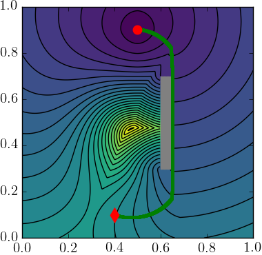
The characteristics of these static PDEs are precisely the optimal trajectories, which define the direction of “information flow”. This is quite useful once (3) is discretized on a grid (e.g., substituting upwind divided differences for partial derivatives, while taking for all gridpoints outside of to enforce the state constraints). The discretization yields a large coupled system of nonlinear equations. Knowing the characteristic direction for every gridpoint, one could, in principle, re-order the equations, effectively decoupling this system. But since the PDE is nonlinear, its characteristic directions are not known in advance. One path11 1 Fast Sweeping [39] is another popular approach for gaining efficiency in solving Eikonal equations. We refer readers to [7, 8] for a review of many other “fast” techniques, including the hybrid marching/sweeping methods that aim to combine the best features of both approaches. Even though our own implementation is based on Fast Marching, any of these methods can be used to solve isotropic control problems arising in subsequent sections. Which one will be faster depends on the domain geometry and the particular pointwise observability functions. to computational efficiency is to determine those characteristic directions simultaneously with solving the discretized system, in the spirit of Dijkstra’s classical algorithm for finding shortest paths on graphs [14]. Two such non-iterative methods (Tsitsiklis’ Algorithm [37] and Sethian’s Fast Marching Method [29]) are applicable to this special isotropic case. Once eq. 3 is solved, the optimal trajectory may be recovered by finding the path orthogonal to the level curves of . This can be achieved numerically by the steepest descent method on . An example of the solution of eq. 3 is shown in 1.

Section 3 Multiple observer locations and different notions of optimality
We now transition to the setting where the observer has a choice of multiple surveillance plans. Assuming that the observer remains stationary, this is equivalent to choosing its position from a fixed set of locations known to the evader. Each location is associated with a pointwise observability function for an evader moving through and an observer stationed at (Typically, is a decreasing function of when is visible from or a small constant if is in a “shadow zone”; see section 5 for further details.) This results in different definitions of the cumulative observability for a particular control. Ideally, a rational evader would prefer a path that minimizes its exposure to all possible observer locations . Unfortunately, there usually does not exist a single control minimizing all ’s simultaneously. This naturally leads us to a notion of Pareto optimal trajectories and the methods for computing them efficiently. We review two such methods22 2 Here we describe these methods in terms of exposure to different observer’s positions, but both of them were introduced for much more general multi-objective control problems. In many applications it is necessary to balance completely different criteria; e.g., time vs fuel vs money vs threat, etc. Other methods for approximating the full PF can be found in [18] and [13]. in section 3.1 and explain how they can be used for planning by an evader optimizing either the worst-case or average-case observability in section 3.2.
Subsection 3.1 Multiobjective path planning
For a fixed starting position , a control is dominated by a control if for all and the inequality is strict for at least one of them. We call Pareto optimal if it is not dominated by any other control. In other words, Pareto optimal controls are the ones that cannot be improved with respect to any one criterion without making them worse with respect to another. The vector of costs associated with each Pareto optimal control defines a point in and the set of all such points is the Pareto Front (PF). In path planning applications, the PF is typically used to carefully evaluate all tradeoffs. (E.g., what is the smallest attainable given the desired upper bounds on ?)
Mitchell and Sastry developed a method for multiobjective path planning[25] based on the usual scalarization approach to multiobjective optimization [23]. Let . For each one can define a new pointwise observability function and a new cumulative observability function . A weighted cost Eikonal equation
| (4) |
is then solved for a fixed , providing a control function satisfying . We call such a control function -optimal. If for all , the obtained -optimal control is also guaranteed to be Pareto optimal; see fig. 2. However, if at least one and multiple -optimal strategies exist for a specific , then some of the -optimal strategies may not be Pareto optimal. Such corner cases (illustrated in fig. 5) might require additional pruning; alternatively, one can rule out such non-Pareto trajectories by perturbing to ensure that all components are positive.
Additional linear PDEs can be solved simultaneously to compute the individual costs incurred along any -optimal trajectory; e.g., when and all ’s are isotropic, the corresponding linear equations are
| (5) |
where
To approximate the PF, this procedure is repeated for a large number of . Unfortunately, as shown in fig. 2, scalarization-based methods can only recover the convex portion of PF [12].
| (A) | (B) |
This is an important drawback since in many optimal control problems the non-convex parts of PF are very common and equally important. An alternative approach was developed in [19] to address this limitation and produce the entire PF for all simultaneously. The method is applicable for any number of observer positions, but to simplify the notation we explain it here for only. We expand the state space to and define the new value function , with the infimum taken over all controls satisfying . Thus, is naturally interpreted as the current “budget” for the secondary criterion. The value function is then recovered by solving an augmented PDE
| (6) |
The method in [19] uses a first-order accurate semi-Lagrangian discretization [16] to compute the discontinuous viscosity solution of (6) for a range of problems in multi-criterion path planning. The method was later generalized to treat constraints on reset-renewable resources [34]. The same approach was also adapted to Probabilistic RoadMap graphs and field-tested on robotic platforms at the United Technologies Research Center [10].
Aside from approximating the entire PF, the key computational advantage is the explicit causality: since is positive, all characteristics are monotone in and methods similar to the explicit “forward marching” in -direction are applicable. (I.e., the system of discretized equations is trivially de-coupled.) Of course, the main drawback of the above idea is the higher dimensionality of . For observer locations, the scalarization approach [25] requires solving PDEs on , but the parameter space is -dimensional. In contrast, with there are no parameters, but the computational domain is -dimensional. Several techniques for restricting the computations to a relevant part of were developed in [19], but the computational cost and memory requirements are still significantly higher than for any (single) HJB-solve in .
Subsection 3.2 Different notions of adversarial optimality
The Pareto Front allows us to answer one version of the surveillance-evasion problem: if the evader is completely risk-averse, he may choose the worst-case optimal strategy. That is, E will pick a control that minimizes the observability from its “worst” observer position :
This corresponds to the version of the problem where E is forced to “go first”, with O selecting the maximizing in response. The following result shows that the intersection of Pareto Front with the “central ray” (i.e., the line where ) yields the worst-case optimal strategy for E:
Theorem 1.
If is a Pareto-optimal control satisfying for all , then is also worst-case optimal.
Proof.
Suppose there exists s.t.
then for all we have:
which contradicts the Pareto-optimality of


The corresponding vector of costs may lie on the convex portion of PF, as in Figures 2(A) and 3, in which case can be found by scalarization [25]. But if lies on the non-convex portion of PF, as in Figures 2(B) and 4, the computational cost of finding the evader’s worst-case optimal strategy grows exponentially with as it involves solving a non-linear differential equation in dimensions [19]. As it will be shown in sections 4-6, the latter scenario is particularly common on domains with obstacles.
Luckily, another interpretation of evader’s objectives proves much more computationally tractable. Even though yields the lowest worst-case observability that E can achieve if he must choose a single control function deterministically, E might be able to attain an even lower expected (or average-case) observability if he switches to “mixed policies”, choosing a probability distribution over a set of Pareto optimal controls. This is illustrated in fig. 2(B): by choosing probabilistically a path corresponding to the point P and another corresponding to point R, E obtains a new point S on the central ray, whose expected observability is lower than for the worst-case optimal Q regardless of O’s selected location. This, of course, assumes that O’s location is selected without knowing in advance which of the two paths will be used by E. Indeed, for any single run from to , the worst-case observability of this probabilistic policy is based on the worst cases for P and R, which (from the point of view of a completely risk-averse evader) would make the average-case optimal S inferior to the worst-case optimal Q. This scenario is fully realized in fig. 4, where , the expected observability corresponding to the optimal “probabilistic mix” of yellow and green trajectories is , but the worst case associated with this mixed policy is .
We note that O could also consider using a mixed strategy. In this case, can be interpreted as the expected pointwise observability when using the probability density over the positions . Similarly is the expected cumulative observability when using the control function . Figure 2 shows that when we are interested in the average-case optimal behavior for both O and E, we only need to consider a convex hull of PF (denoted ), and the scalarization is thus adequate. Note that in figs. 3, 4, and 6, the set was approximated by imposing a fine grid on and re-solving eq. 4 for each sampled Since we only care about the intersection of with the central ray, this procedure is wasteful – and prohibitively expensive for high . In the next section, we consider the case where both E and O optimize the expected/average-case performance by reformulating this as a semi-infinite strategic zero-sum game. We show that such Surveillance-Evasion Games (SEGs) can be solved through scalarization combined with convex optimization, without approximating the (convex hull of the) entire Pareto Front.
Remark 2.
Up till now, our geometric interpretation in figs. 3, 4, and 6 assumed that either PF or at least the must intersect the central ray. If this is not the case, O will avoid using some of his positions. E.g., fig. 5 shows the pink and yellow trajectories corresponding to and , which are optimal with respect to the observer positions and . Since the E’s worst-case for is actually the observer location . A generalization of this scenario for is covered in theorem 4.


Section 4 Surveillance-Evasion Games (SEGs)
In this section, we reformulate the problem of evasive path planning under surveillance uncertainty as a strategic game. This can model either the actual adversarial interactions between two players or the risk-averse logic of the evader even if the surveillance patterns are not likely to change in response to that evader’s strategy. (The latter case is typically interpreted as a “game against nature”.)
We assume that the evader is attempting to minimize (while the observer is attempting to maximize) the total expected observability integrated over E’s trajectories and dependent on O’s positions. We further assume that O is aware of E’s initial location and its target location but not of the trajectories chosen by E. Similarly, E is aware of the predefined locations of O, but not of the realized positions chosen by O. This game may be stated deterministically or stochastically. In the deterministic case, each player chooses a single pure strategy. That is, the observer chooses a single location and the evader chooses a single control function . In the probabilistic setting, each player chooses a mixed strategy, i.e., a probability distribution over the pure strategies. In other words, O chooses a probability distribution over positions and E chooses a probability distribution over control functions. The mixed strategy of the observer can be interpreted in several different ways:
- 1.
O chooses a single position according to the probability distribution before E starts moving, and remains at that position until the end of the round (that is, until E reaches the target).
- 2.
O can randomly teleport between its positions at any time, and each reflects the proportion of time spent at the corresponding position .
- 3.
O has a budget of “observation resources”, and reflects the fraction of these resources spent at each location. In this case, reflects the pointwise observability corresponding to 100% of resources allocated to the position .
Since we assume that neither player has access to the realization of the opponent’s strategy in real time, these three interpretation are equivalent (and lead to the same optimal strategies) in our context. The payoff function of the game is the cumulative expected observability, and can be expressed as where denotes the expectation over the mixed strategy .
This SEG is a two-player zero-sum game [26], as each player’s gains or losses are exactly balanced by the losses or gains of the opponent. Furthermore, it is semi-infinite as the set of pure strategies for O is a finite number , whereas the set of pure strategies for E is uncountably infinite. A central notion of solution for strategic games is a Nash equilibrium [26], a pair of strategies for which neither player can improve his payoff by unilaterally changing his strategy. That is, a pair of strategies is a Nash equilibrium if both of the following conditions hold:
| (7) | ||||
A pure strategy Nash equilibrium does not always exist, therefore we focus on finding a mixed strategy Nash equilibrium. In our setting, the minimax theorem for semi-infinite games [28] assures that a mixed strategy Nash equilibrium exists, that all Nash equilibria have the same payoff, and that they are attained at the minimax (which is also equal to the maximin):
| (8) |
Although is a probability distribution over the uncountable set , there always exists an optimal mixed strategy which is a mixture of at most pure strategies, where is the maximum number of positions for the observer [28]. In fact, it is easy to show that there will always exist a Nash equilibrium with the number of pure strategies used in not exceeding the number of non-zero components in
In the case of finite two-player zero-sum games, computing the Nash equilibrium is easily achieved by linear programming. For our SEGs, the challenge in computing a Nash equilibrium arises from enumerating the control functions which are part of E’s mixed strategy. Indeed, we do not possess a useful parametrization of the set of control functions , and our only computational kernel to generate a single -optimal control function is to solve the weighted-cost Eikonal equation in eq. 4. For that reason, our solution strategy to compute the Nash Equilibrium involves two steps:
- 1.
Find an approximate optimal strategy of the observer using convex optimization (see section 4.1).
- 2.
Find an approximate optimal strategy of the evader by generating near-optimal control functions (see section 4.2).
Subsection 4.1 Optimal strategy of the Observer
In order to compute an optimal strategy of the observer, we consider the following problem:
| (9) |
For any fixed strategy for O, the inner minimization represents the optimal response of player E to that fixed strategy. Therefore, the maximin problem answers the question: what is the optimal strategy for O given that E gets to observe that strategy and respond? We call this problem the E-response problem. Note that although E could use a mixed strategy, there always exists a pure strategy which is optimal. That is:
| (10) |
This implies that any optimal for eq. 9 is also an optimal for eq. 8. Consequently, the optimal for eq. 9 is one half of a Nash equilibrium pair. However, the optimal pair of eq. 9 is not a Nash equilibrium, except in a specific situation described in the following theorem.
Theorem 3.
Suppose there exists with associated -optimal control function which satisfies for all , then is a Nash equilibrium.
Proof.
The fact that E cannot improve his payoff follows from the definition of . O may not improve his payoff either as for all ,
This situation corresponds to the case when the convex part of the Pareto Front intersects the central ray, such as in the example in fig. 3. Theorem 1 implies that in this case, the worst-case optimal strategy for E coincides with E’s half of the Nash equilibrium. Note that in general such a does not have to exist; e.g., in fig. 4 and fig. 6 the convex part of the Pareto Front does not intersect the central ray. In such situations, the worst-case optimal strategy for E and the Nash Equilibrium are different. Moreover, the latter involves a mixed strategy for E covered in section 4.2.
We now direct our attention to solving the E-response problem numerically. Equation 9 may be stated as the following optimization problem:
| (11) | ||||
The objective function is concave as it is the pointwise minimum of linear functions. Furthermore, the vector of individual cumulative costs , where , is a supergradient of (denoted as ). A supergradient provides an ascent direction of a concave function, i.e., if for all ,
The fact that is seen from the following computation: for any ,
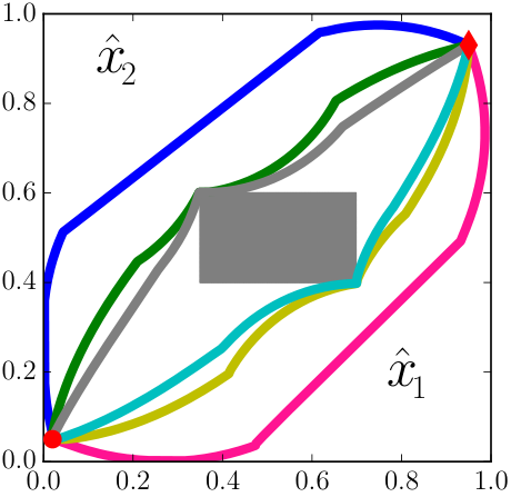
Evaluating the vector can be challenging computationally; we show how this can be done in section 5.2. Once this ascent direction is known, one still needs to ensure that remains a feasible probability distribution over , and we use the orthogonal projection operator . The operator can be computed in operations [4, 38] as summarized in algorithm 1. The resulting projected supergradient method [3, Chap. 8] is shown in algorithm 2. The iterates of algorithm 2 for the example from fig. 6 are illustrated in fig. 7.


Subsection 4.2 Optimal strategy of the Evader
Computing the evader’s half of the Nash equilibrium is more challenging due to the fact that the set of E’s pure strategies, i.e., the set of control functions leading from the source to the target , is uncountably infinite. We propose a heuristic strategy to approximate which relies on two properties of the Nash equilibrium in semi-infinite games:
- 1.
There exists a Nash mixed strategy for E which uses only pure strategies33 3 This result assumes that the set is bounded and is closed. In our case, is not bounded for the full set of control functions in but becomes bounded if we restrict our attention to Pareto optimal control functions. [28].
- 2.
All pure strategies employed with positive probability in the Nash equilibrium have the same expected payoff, with the expectation taken over the other half of the Nash. In particular, all control functions used with positive probability in the Nash equilibrium are -optimal.
The following characterization of the Nash equilibrium helps us generate a good candidate set of -optimal trajectories.
Theorem 4.
Let and . is a Nash equilibrium if and only if the following three conditions hold:
- 1.
is a constrained maximizer of in eq. 11,
- 2.
if then , and
- 3.
if , then .
Proof.
( )
Suppose is a Nash equilibrium. Item 1 follows from the minimax theorem for semi-infinite game and eq. 10. Assume item 2 does not hold, then there must exist s.t. . Consider the strategy :
Then we have that:
This contradicts that is a Nash equilibrium, thus item 2 must hold. A similar argument can be used to demonstrate item 3: assume there exists with . Let and consider the strategy :
Once again, this implies that which contradicts that is a Nash equilibrium.
() Assume items 1, 2, and 3 hold and suppose there exists s.t. , then there must exist , used with non-zero probability in such that:
This contradicts the definition of . Thus, for all we have that:
| (12) |
From items 2 and 3 it follows that for all :
| (13) |
Equations 12 and 13 imply that is a Nash equilibrium.
Any mix of -optimal trajectories forms a -optimal strategy for the evader. However, that mix is part of a Nash equilibrium only if the observer has no incentive to change his strategy in response. Theorem 4 says that this is the case when the defining the mix of individual observability of -optimal trajectories lies on the central ray of the Pareto Front for a reduced problem. I.e., the PF for the SEG where the observer has a potentially smaller number of positions (the ones which are used with positive probability in ). This PF is in an dimensional criterion space, where . In fig. 3, the number of observer positions is , and the dimension of the “reduced” problem is also since both positions are used with positive probability. In this example, a single -optimal trajectory exists and corresponds to the intersection of the central ray and the convex part of the PF. In the examples from fig. 4 and fig. 6, we still have and , however there are two -optimal trajectories. The Nash mixed strategy for E is thus obtained by finding a probability distribution over these two trajectories such that the linear combination of their individual costs lies on the central ray, i.e., such that . In the example from fig. 5, and . The PF of the reduced problem is a single point, and thus trivially lies on the “central ray”, yielding a pure Nash equilibrium strategy for E. In section 5, we show additional examples with , , and , . Computationally, Theorem 4 means that if we are able to find a set of -optimal control functions , such that items 2 and 3 hold for some probability distribution , then is O’s optimal response to and we have found a Nash equilibrium pair. Note that the minimum number of trajectories needed to form a Nash equilibrium is bounded above by .
One remaining task is finding such a set . Multiple -optimal controls only exist if lies on a shockline of , where the gradient is undefined (e.g., the can be different depending on the sequence ). Numerically, our approximation of will yield a single upwind approximation of yielding a single -optimal trajectory. As we show in fig. 8, multiple optimal trajectories might lie in the same upwind quadrant and any numerical implementation of gradient descent will find only one of them. (In theory, one can approximate the other by perturbing , but the direction of perturbation is unobvious, particularly when lies on an intersection of multiple shocklines, which is surprisingly common in this application as we show in further sections.)


This challenge is even more pronounced because 2 yields an approximate value of , since will now be only near a shockline for some perturbed . The resulting single -optimal control will be a reasonable approximate solution for the max-min problem, but can be arbitrarily far from the solution to a min-max problem (where O has a chance to switch to another strategy).
In view of these challenges, we opt for a different approach, where an approximation to is computed iteratively, by adaptively growing a collection of -optimal controls corresponding to different ’s. In some degenerate cases, generating even the first may not be trivial since some -optimal control computed by solving the Eikonal will not be necessarily Pareto-optimal. E.g., in fig. 5 two control functions are -optimal, but only one of them is used in the Nash strategy of E as the blue trajectory violates item 3. However, both trajectories are indistinguishable from the point of view of the Eikonal solver since the position has zero weight in the weighted observability function . To address this issue whenever , we set the weight of the pointwise observability of each unused position to some small value (our implementation uses ). This is equivalent to seeking the solution of the weighted cost Eikonal equation for some perturbed , where is the characteristic function of the complement of . We now turn our attention to finding further perturbations needed to generate -optimal trajectories in order to make item 2 approximately hold. Our goal is to have
| (14) |
approximately hold for all . Unless this is already true with (based on the previously found ), we will need to find more -optimal controls. Without loss of generality assume that , and suppose we have already generated a set of -optimal trajectories , for some . In order for eq. 14 to approximately hold, we will be increasing until the norm of residual
| (15) |
falls under a threshold . Assuming the set of trajectories has already been computed, the probability distribution minimizing the norm of this residual can be found by quadratic programming. The residual vector provides information about which control functions are missing. For example, consider the case where we observe that a single entry of is large and positive, i.e., that for some :
The characterization in theorem 4 implies that should include at least one trajectory much more observable from position . A -optimal trajectory with that property can be found by perturbing to slightly decrease the role of in O’s chosen strategy. This is equivalent to re-solving the Eikonal with corresponding to where is chosen adaptively (see algorithm 4), is the -th standard basis vector, and is the orthogonal projection onto the simplex defined only with elements of . Once a new -optimal control function has been found, we may solve the quadratic program in eq. 15 again with an additional column, and repeat the process until the norm of the residual is sufficiently small. More generally, a large implies that some control functions in (or some mix of control functions) not in the current set has a high observability with respect to the positive entries of while having a low observability with respect to the negative entries of . Thus, we set the perturbation direction to instead of . Throughout this perturbation step, the entries of associated with the complement are held fixed. Our full method for computing an approximate Nash equilibrium is summarized in algorithm 3.
This method also has a geometric interpretation in terms of the Pareto Front. Whenever is not a pure strategy, a hyperplane normal to supports PF at multiple points (corresponding to all controls in ). However, any generic perturbation of would result in a hyperplane supporting PF near only one of these points, and the approximation to found by algorithm 2, will correspond to a single optimal trajectory. For example, if we start with corresponding to the yellow point in fig. 6c (and associated yellow trajectory in fig. 6b), then a small tilt (decreasing the role of position in O’s plan) will yield a hyperplane supporting PF near the green point, allowing us to approximate the green trajectory in fig. 6b by solving the weighted cost Eikonal equation with observability function .
Section 5 Numerical matters
In this section, we detail the implementation of our algorithm and present additional numerical results. All algorithms were implemented in C++ and compiled with icpc version 16.0 on a MacBook Pro (16 GB RAM and an Intel Core i7 processor with four 2.5 GHz cores). The code is available online at https://github.com/eikonal-equation/Stationary_SEG. Our implementation relies on data structures and methods from Boost, Eigen and QuadProg++ libraries.
Subsection 5.1 Functions, parameters, methods
All of our examples are posed on the domain with the possible exclusion of obstacles. All figures are based on computations on a uniform cartesian grid of size (with the grid spacing ). To simplify the discussion, we always use a constant speed function though any inhomogeneous speed can be similarly handled by solving the Eikonal equation eq. 3.
The pointwise observability functions are defined as
We set and with in all examples except in fig. 5 (where we set simply to improve the visualization). The visibility of each gridpoint with respect to each observer position is precomputed and stored, but the values are computed on the fly as needed.
The shadow zones for each observer are precomputed as follows. For each observer location , two distance functions are computed: and . The first is the distance between and when the obstacles are absent, while the second is that distance when obstacles are present. These distance functions can be computed by imposing the boundary conditions and then solving two Eikonal equations [30]:
| (16) |
with set to inside the obstacles and otherwise. The shadow zone of is characterized by . But due to numerical errors in their approximation, we use a threshold value (where is the grid spacing) and specify that is in this shadow zone whenever
The perturbation stepsize in algorithm 3 is chosen adaptively using algorithm 4. The goal of the adaptive strategy is to find the smallest perturbation necessary to obtain an additional -optimal control function .
The initialization used in our implementation is , and the tolerance is set to . The stepsize rule used in the supergradient iteration in algorithm 2 is , the initial guess is a uniform distribution on and the tolerance criteria on the residual and the near entries used in algorithm 3 are and respectively. The quadratic programming problem in eq. 15 is solved using the library QuadProg++.
Subsection 5.2 Computation of individual costs
Running algorithm 2 requires computing the vector of individual observability . This problem is exactly the one solved by the scalarization approach described in section 3.1. Therefore, it can in principle be done by solving the Eikonal equation in eq. 3 with cost function and associated linear equations in eq. 5; i.e.: and . However, this technique has a severe drawback for this particular application: at the optimal , is often discontinuous at . E.g., in fig. 8b, the upwind stencil containing the two -optimal trajectories contains a point on either side of the discontinuity line of (which is the shockline of ). As a result, the value of is updated by interpolating the discontinuous function across the line of discontinuity.
This effect happens when multiple trajectories are -optimal. Each of these trajectories has the same expected cumulative observability , but different individual observability . This issue leads to a large numerical error when using to estimate the supergradient in algorithm 2, causing poor convergence of the method. Instead, we use the following process to compute the individual costs: first we solve the weighted cost Eikonal equation eq. 4 to obtain for a fixed , then we trace the path using a gradient descent method on the value function and numerically estimate the integrals:
Subsection 5.3 Additional experiments and error metrics
We present two additional examples that include a higher number of observer plans. In fig. 9, we show an example where the mixed strategy Nash equilibrium consists of a distribution over three strategies for both the evader and the observer. Figure 9 shows the value function at the optimal . We observe that three shocklines of the value function meet at the source location , which implies that four trajectories are optimal starting from this location. However, the minimax theorem for infinite games assures that only 3 pure strategies are necessary to form a Nash equilibrium. Using algorithm 3, we find an approximate Nash equilibrium which uses a mix of such three trajectories.

In Figure 10, we show a maze-like example where the observer may choose among six possible positions. Using algorithm 3, we determine that at the approximate Nash equilibrium, only four positions are used with positive probability by O, and E uses four different trajectories which are displayed in fig. 10.

In order to test the performance of algorithm 3, we consider three error metrics:
- 1.
The optimization error in arises from several effects: the discretization error of the Eikonal solver, the discretization error of the path tracing and path integral evaluation, and the early stopping of the supergradient iterations. To generate the “ground truth”, we performed the same computation on a finer grid of size of (i.e. we consider a grid with 16 times more unknowns) and run the supergradient iteration until we observe stagnation in the objective function value of the iterates. We approximate the relative error in our computations on a grid as:
- 2.
The Observer’s regret estimates how much the observer could improve his payoff by unilaterally deviating from our approximate Nash equilibrium. (Recall that, if the approximate Nash equilibrium were exact, the observer would not be able to increase his payoff at all). We quantify this error using the normalized residual in eq. 15, i.e.:
- 3.
The Evader’s regret estimates how much the evader could improve his payoff by unilaterally deviating from our approximate Nash equilibrium. This corresponds to how far from -optimal are the controls produced by algorithm 3. Recall that the control function is (up to numerical errors) -optimal, whereas for are -optimal. We report the maximum relative error in cumulative observability of the -optimal trajectories, that is:
These error metrics are reported in table 1 along with timing metrics for each example presented in the paper.
Section 6 Extension to groups of evaders
We now consider an extension of the surveillance-evasion game to a game which involves a team of evaders. Each evader chooses a trajectory leading him from his own source location to a target location , according to his own speed function . The pointwise observability function is shared for all evaders and depends only on the strategy of the observer. This induces different cumulative observability functions defined as in eq. 1, and different value functions which are solutions of Eikonal equations with different boundary conditions.
In this version of the game, we assume that a central organizer for evaders faces off against the observer. The goal of that central organizer is to minimize the weighted sum of evaders’ cumulative expected observabilities. The weights in the sum reflect the relative importance of each evader. We further assume that the central organizer and the observer agree on that relative importance, making this a two player zero-sum game with a payoff function defined by:
| (17) |
Although we focus on a zero-sum two player game, we note that its Nash equilibrium must also be among Nash equilibria of a different -player game: the one, where each of the evaders is selfishly minimizing their own cumulative observability , while the observer still attempts to maximize the crowd-wide observability in eq. 17. This property follows from two simple facts:
- 1.
The Observer’s payoff is the same in both versions of the game and thus cannot be improved unilaterally in a player game.
- 2.
In the Nash equilibrium for the two-player game, the central organizer would only ask each evader to assign positive probabilities to their -optimal trajectories. (Otherwise, the weighted sum in eq. 17 could be improved). Thus, they would also be maximizing their individual payoffs.
In this new setting, theorem 4 holds and the observer’s half of the Nash equilibrium may be found by maximizing the concave function:
| (18) |
The function and its supergradients may be evaluated in a similar way to section 5.2, but require solves of the Eikonal equation with different boundary conditions and speed functions, and the numerical evaluation of path integrals. However, we note that if all evaders have the same speed function and share the same target location (or, alternatively, share the same source location), only a single Eikonal equation solve is in fact required. With minor modifications, algorithm 3 may be also applied to solve this version of the problem. For each perturbation of a set of control functions is generated on line 8 of algorithm 3, with one control function found for each evader. Although we obtain a new set of control functions for each perturbation, some of the control functions for specific evaders may be essentially the same as those already obtained from previous perturbations. We address this in post-processing, by pruning the output of modified algorithm 3 to identify distinct trajectories for each evader.
We show numerical results for two test problems with equally important evaders (i.e., ) in each of them. An example presented in fig. 11 uses the same obstacle and the same possible observer locations already used in fig. 6. At the approximate Nash equilibrium found using algorithm 3, the observer uses these two locations with probabilities and the central controller directs both evaders to use pure policies: deterministically choose pink and blue trajectories to their respective targets. Even though the first evader’s starting position and destination are also the same as in fig. 6, his (and the Observer’s) optimal strategies are quite different here due to the second evader’s participation.


In a maze-like example presented in fig. 12, O can choose among six possible locations, but his optimal mixed strategy uses only four of them. algorithm 3 yields three sets of two near--optimal trajectories which form an approximate Nash equilibrium, but they only contain two distinct trajectories for each of the evaders. We report timing and error metrics for these two examples in table 2.


| fig. 11 | fig. 12 | |
|---|---|---|
| Number of it. of algorithm 2 | 353 | 300 |
| Total CPU time (seconds) | 631 | 594 |
| Observer’s regret | ||
| Evader’s regret |
Section 7 Conclusion
We have considered an adversarial path planning problem, where the goal is to minimize the cumulative exposure/observability to a hostile observer. The current position of the latter is unknown, but the full list of possible positions is assumed to be available in advance. The key assumption of our model is that neither the Evader (E) nor the enemy Observer (O) can adjust their plan in real time based on the opponent’s state and actions. Instead, both of them are required to choose their (possibly randomized) strategies in advance. We discussed two versions of this problem; in the first one, a completely risk-averse evader attempts to minimize his worst-case cumulative observability. We showed that this version can be solved using previously developed methods for multiobjective path planning. However, the solution is prohibitively computationally expensive when O has a large number of surveillance plans to choose from. In the second version, the subject of optimization is the E’s expected cumulative observability on its way to the target. We modeled this as a zero-sum Surveillance-Evasion Game (SEG) between two players: E (the minimizer) and O (the maximizer). We then presented an algorithm combining ideas from continuous optimal control, the scalarization approach for multiobjective optimization, and convex optimization which allows us to quickly compute an approximate Nash equilibrium of this semi-infinite strategic game. Finally, we showed that this algorithm extends to solve a similar problem involving a group of multiple evaders controlled by a central planner. The presented algorithm displays at most linear scaling in the number of observation plans, but further speed up techniques would be desirable; the computational bottleneck (numerically solving the Eikonal equation) could be alleviated with domain restriction methods [9] and factoring approaches [27].
Although this paper focused on isotropic problems, the anisotropic observer case could be treated in a similar fashion. (In practice, the pointwise observability might depend on the angle between the evader’s direction of motion and the observer’s line of sight.) This generalization will have to rely on fast numerical methods developed for anisotropic HJB PDEs; e.g., [31, 1, 24, 36]. In a follow-up paper [6], we show that time-dependent observation plans (e.g., different patrol routes) can be similarly treated by solving -parametrized finite-horizon optimal control problems with numerical methods for time-dependent HJB equations; e.g., [16, 32].
We note that the computational cost of our algorithm increases quickly with the number of evaders considered. The case involving a large number of selfish evaders could be covered by considering the evolution of a time-dependent density of observers, and treating the problem using mean field games [17, 5]. Another possible extension would be to consider a group of observers choosing among a larger set of surveillance plans. In that situation, the set of pure strategies of the observers could increase exponentially, but we anticipate that the computational cost will grow much slower since the number of required Eikonal solves would not increase.
Acknowledgements: The authors would like to thank Alex Townsend and anonymous reviewers for their helpful suggestions.
References
- [1] K. Alton and I. M. Mitchell, An ordered upwind method with precomputed stencil and monotone node acceptance for solving static convex Hamilton-Jacobi equations, Journal of Scientific Computing, 51 (2012), pp. 313–348.
- [2] M. Bardi and I. Capuzzo-Dolcetta, Optimal control and viscosity solutions of Hamilton-Jacobi-Bellman equations, Springer Science & Business Media, 2008.
- [3] A. Beck, First-Order Methods in Optimization, vol. 25, SIAM, 2017.
- [4] P. Brucker, An algorithm for quadratic knapsack problems, Operations Research Letters, 3 (1984), pp. 163–166.
- [5] R. Carmona and F. Delarue, Probabilistic Theory of Mean Field Games with Applications I-II, Springer, 2017.
- [6] E. Cartee, L. Lai, Q. Song, and A. Vladimirsky, Time-dependent surveillance-evasion games, preprint arXiv:1903.01332, (2019).
- [7] A. Chacon and A. Vladimirsky, Fast two-scale methods for eikonal equations, SIAM Journal on Scientific Computing, 34 (2012), pp. A547–A578.
- [8] , A parallel two-scale method for eikonal equations, SIAM Journal on Scientific Computing, 37 (2015), pp. A156–A180.
- [9] Z. Clawson, A. Chacon, and A. Vladimirsky, Causal domain restriction for eikonal equations, SIAM Journal on Scientific Computing, 36 (2014), pp. A2478–A2505.
- [10] Z. Clawson, X. Ding, B. Englot, T. A. Frewen, W. M. Sisson, and A. Vladimirsky, A bi-criteria path planning algorithm for robotics applications, preprint arXiv:1511.01166, (2015).
- [11] M. G. Crandall and P.-L. Lions, Viscosity solutions of Hamilton-Jacobi equations, Transactions of the American Mathematical Society, 277 (1983), pp. 1–42.
- [12] I. Das and J. E. Dennis, A closer look at drawbacks of minimizing weighted sums of objectives for Pareto set generation in multicriteria optimization problems, Structural optimization, 14 (1997), pp. 63–69.
- [13] A. Desilles and H. Zidani, Pareto front characterization for multi-objective optimal control problems using Hamilton-Jacobi approach, preprint, (2018).
- [14] E. W. Dijkstra, A note on two problems in connexion with graphs, Numerische mathematik, 1 (1959), pp. 269–271.
- [15] J. Dobbie, Solution of some surveillance-evasion problems by the methods of differential games, in Proceedings of the 4th International Conference on Operational Research, MIT, John Wiley and Sons, New York, New York, 1966.
- [16] M. Falcone and R. Ferretti, Semi-Lagrangian approximation schemes for linear and Hamilton-Jacobi equations, vol. 133, SIAM, 2014.
- [17] O. Guéant, J.-M. Lasry, and P.-L. Lions, Mean field games and applications, in Paris-Princeton lectures on mathematical finance 2010, Springer, 2011, pp. 205–266.
- [18] A. Guigue, Approximation of the pareto optimal set for multiobjective optimal control problems using viability kernels, ESAIM: COCV, 20 (2014), pp. 95–115.
- [19] A. Kumar and A. Vladimirsky, An efficient method for multiobjective optimal control and optimal control subject to integral constraints, Journal of Computational Mathematics, (2010), pp. 517–551.
- [20] J. Lewin, Decoy in pursuit-evasion games, PhD thesis, Department of Aeronautics and Astronautics, Stanford University, 1973.
- [21] J. Lewin and J. V. Breakwell, The surveillance-evasion game of degree, Journal of Optimization Theory and Applications, 16 (1975), pp. 339–353.
- [22] J. Lewin and G. J. Olsder, Conic surveillance evasion, Journal of Optimization Theory and Applications, 27 (1979), pp. 107–125.
- [23] R. T. Marler and J. S. Arora, Survey of multi-objective optimization methods for engineering, Structural and multidisciplinary optimization, 26 (2004), pp. 369–395.
- [24] J.-M. Mirebeau, Efficient fast marching with Finsler metrics, Numerische mathematik, 126 (2014), pp. 515–557.
- [25] I. M. Mitchell and S. Sastry, Continuous path planning with multiple constraints, in Decision and Control, 2003. Proceedings. 42nd IEEE Conference on, vol. 5, IEEE, 2003, pp. 5502–5507.
- [26] M. J. Osborne and A. Rubinstein, A course in game theory, MIT press, 1994.
- [27] D. Qi and A. Vladimirsky, Corner cases, singularities, and dynamic factoring, Journal of Scientific Computing, 79 (2019), pp. 1456–1476.
- [28] T. Raghavan, Zero-sum two-person games, Handbook of game theory with economic applications, 2 (1994), pp. 735–768.
- [29] J. A. Sethian, A fast marching level set method for monotonically advancing fronts, Proceedings of the National Academy of Sciences, 93 (1996), pp. 1591–1595.
- [30] J. A. Sethian, Level set methods and fast marching methods: evolving interfaces in computational geometry, fluid mechanics, computer vision, and materials science, vol. 3, Cambridge university press, 1999.
- [31] J. A. Sethian and A. Vladimirsky, Ordered upwind methods for static Hamilton–Jacobi equations: Theory and algorithms, SIAM Journal on Numerical Analysis, 41 (2003), pp. 325–363.
- [32] C.-W. Shu, High order numerical methods for time dependent Hamilton-Jacobi equations, in Mathematics and computation in imaging science and information processing, World Scientific, 2007, pp. 47–91.
- [33] H. Soner, Optimal control with state-space constraint. I, SIAM Journal on Control and Optimization, 24 (1986), pp. 552–561.
- [34] R. Takei, W. Chen, Z. Clawson, S. Kirov, and A. Vladimirsky, Optimal control with budget constraints and resets, SIAM Journal on Control and Optimization, 53 (2015), pp. 712–744.
- [35] S. Tijs, Semi-infinite linear programs and semi-infinite matrix games, Katholieke Universiteit Nijmegen. Mathematisch Instituut, 1976.
- [36] Y.-H. R. Tsai, L.-T. Cheng, S. Osher, and H.-K. Zhao, Fast sweeping algorithms for a class of Hamilton–Jacobi equations, SIAM Journal on Numerical Analysis, 41 (2003), pp. 673–694.
- [37] J. N. Tsitsiklis, Efficient algorithms for globally optimal trajectories, IEEE Transactions on Automatic Control, 40 (1995), pp. 1528–1538.
- [38] W. Wang and M. A. Carreira-Perpinán, Projection onto the probability simplex: An efficient algorithm with a simple proof, and an application, arXiv preprint arXiv:1309.1541, (2013).
- [39] H. Zhao, A fast sweeping method for eikonal equations, Mathematics of computation, 74 (2005), pp. 603–627.