Relaxation by thermal conduction of a magnetically confined mountain on an accreting neutron star–?

During accretion, the neutron star’s polar magnetic field buckles underneath the infalling matter, and the field lines spread equatorially due to flux freezing. The lateral pressure gradient at the base of the accreted mountain is balanced by the Lorentz force in the compressed, equatorial magnetic belt. This process is illustrated schematically in Figure 1 [see also Figure 6 of Priymak et al. 2011]. The compressed magnetic field is more intense than the pre-accretion field locally, due to magnetic flux conservation, but the global moment $\mu$ reduces, because the magnetic distortion induces screening currents, which reduce the radial magnetic field near the pole (Vigelius & Melatos 2008; Mastrano & Melatos 2012).

It is observed that $\mu$ decreases with $M_{a}$ in binary systems (Taam & van den Heuvel 1986; van den Heuvel & Bitzaraki 1995; Zhang & Kojima 2006). Shibazaki et al. 1989 proposed the widely used, empirical law

In (1), we define $M_{c}$ to be the critical accreted mass, for which the global dipole moment is halved. The dipole moment before accretion begins is given by $\mu_{i}=B_{\star}R_{\star}^{3}$. We take $R_{\star}=10^{6}\text{ cm}$ for the stellar radius and $B_{\star}=10^{12.5}\textrm{ G}$ for the natal magnetic field strength at the polar surface, in line with population synthesis models (Arzoumanian et al. 2002; Faucher-Giguère & Kaspi 2006). Self-consistent, MHD simulations reproduce the empirical scaling (1) for small accreted masses $M_{a}\ll M_{c}$ in isothermal and adiabatic mountains with $M_{c}\sim 10^{-6}M_{\odot}$ and $M_{c}\sim 10^{-8}M_{\odot}$ respectively (Payne & Melatos 2004; Vigelius & Melatos 2009a; Priymak et al. 2011). For $10^{-1}\lesssim M_{a}/M_{c}\lesssim 10$, the simple estimate in (1) breaks down and the burial effect is better represented by a power-law $\mu/\mu_{i}=(M_{a}/M_{c})^{-a}$, where $1\leq a\leq 2.47$ depends on the EOS [see section 4.1 of Priymak et al. 2011 and Fig. 8(c) of Payne & Melatos 2004]. Numerical difficulties prevent simulations from probing the regime $M_{a}/M_{c}\gtrsim 10$, where a significant deviation from (1) is expected (Haskell et al. 2015), though Ohmic diffusion sets a burial limit of $\mu/\mu_{i}\gtrsim 10^{-8}$ (Vigelius & Melatos 2009b).

The critical mass $M_{c}$ depends strongly on the EOS (Priymak et al. 2011). For a softer EOS, the mountain has a relatively small thickness $(H_{\text{max}}\sim 10^{3}\text{ cm})$, because the material is easier to compress. Strong local magnetic fields $(\lesssim 10^{15}\text{ G})$ exist near the stellar surface, as polar field lines buckle, and the polar magnetic flux is squeezed into a small volume. Consequently, the screening currents flow closer to the stellar surface for a softer EOS than for a harder EOS, and $\mu$ reduces less for a given $M_{a}$. For a softer EOS, the critical mass is found to lie in the range $10^{-5}\lesssim M_{c}/M_{\star}\lesssim 10^{-2}$ (Payne & Melatos 2004). For a harder EOS, the mountain is thicker $(H_{\text{max}}\sim 10^{4}\text{ cm})$, and $\mu$ reduces further. For a polytropic EOS with index $\Gamma\gtrsim 4/3$, the critical mass is found to lie in the range $10^{-9}\lesssim M_{c}/M_{\star}\lesssim 10^{-6}$ (Priymak et al. 2011). Priymak et al. 2011 found $M_{c}\propto B_{\star}^{2}$.

The mountain mass quadrupole moment can be expressed in terms of the mass ellipticity $\epsilon$, which is given approximately by (Melatos & Payne 2005)

where $M_{\star}=1.4M_{\odot}$ is the stellar mass. Therefore, for a given accreted mass, there is a one-to-one relationship between $\mu$ and $\epsilon$ through (1) and (2) which depends on the value of $M_{c}$. The mass quadrupole moment emits gravitational radiation, as the star spins (Melatos & Payne 2005). The implications are discussed in Section 4.2.

The hydromagnetic structure of the mountain has been calculated for various EOS previously (Payne & Melatos 2004; Payne & Melatos 2006a; Vigelius & Melatos 2008; Priymak et al. 2011; Mukherjee et al. 2013a). In this paper, we start by solving for the structure of a steady-state $(\partial/\partial t=0)$ and immobile ($\boldsymbol{v}=0$, where $\boldsymbol{v}$ is the fluid velocity) mountain. We then input the result into PLUTO as the starting point for time-dependent simulations which include thermal conduction. In the first stage we do not model growth of the mountain but rather solve for a self-consistent equilibrium (i.e. hydromagnetic force balance) given a certain amount of accreted mass and an EOS. Time-dependent simulations in the literature confirm that the equilibrium agrees closely with mountains built from scratch by injecting mass from below (Vigelius & Melatos 2009c; Wette et al. 2010).

We assume that the magnetic field $\boldsymbol{B}$ may be described through an axisymmetric Chandrasekhar decomposition without a toroidal component¹¹ 1 Three-dimensional mountain equilibria for $M_{a}\gtrsim M_{c}$ are susceptible to Parker-like (Vigelius & Melatos 2008) and ballooning (Mukherjee et al. 2013b) instabilities with EOS-dependent growth rates (Kosiński & Hanasz 2006). However, the instabilities do not disrupt the mountain; they reduce the ellipticity by $\lesssim 30$ percent when they saturate (Vigelius & Melatos 2008). Furthermore, previous three-dimensional, time-dependent simulations reveal that the magnetic field relaxes to an almost axisymmetric configuration within a few Alfvén times (Payne & Melatos 2007; Vigelius & Melatos 2008). for simplicity, i.e. $\boldsymbol{B}$ takes the form

in spherical coordinates $\left(r,\theta,\varphi\right)$, where $\psi(r,\theta)$ is a scalar flux function (Chandrasekhar 1956). The mountain equilibrium is determined by the force balance (Grad-Shafranov) equation (Payne & Melatos 2004; Mukherjee & Bhattacharya 2012)

where $\Delta^{2}$ denotes the Grad-Shafranov operator,

$p$ is the fluid pressure, $\rho$ is the mass density, and $\phi$ is the gravitational potential. For now, we assume that the accreted matter obeys a barotropic EOS, $p=p(\rho)$, once equilibrium is reached. Although neutron stars are expected to be non-barotropic (Goldreich & Reisenegger 1992), the barotropic and non-barotropic solutions to the Grad-Shafranov problem are broadly similar, even in magnetars (Mastrano et al. 2011; Mastrano et al. 2015).

For $p=p(\rho)$, equation (4) implies that $\rho$ and $\psi$ satisfy

Equation (6) can be solved exactly using the Lagrange-Charpit method to yield (Courant & Hilbert 1953)

where $\phi_{0}$ denotes a reference gravitational potential at the neutron star surface, and $F$ is an arbitrary function of the scalar flux. Given $p=p(\rho)$, the integral in (7) can be evaluated, in principle, to express $\rho$ in terms of $\psi$ or vice-versa.

In order to obtain a one-to-one correspondence between the pre- and post-accretion states that respects flux-freezing, we demand that the steady-state, mass-flux ratio $dM/d\psi$, defined as the mass enclosed between the infinitesimally separated flux surfaces $\psi$ and $\psi+d\psi$, equals that of the initial state plus any accreted matter (Alfvén 1943; Mouschovias 1974; Melatos & Phinney 2001). This restriction on $M(\psi)$ leads to the constraint (Payne & Melatos 2004)

where $C$ is the curve $\psi[r(s),\theta(s)]=\psi$ parametrized by the arc length $s$. Equation (8) can be solved by inverting (7) for $\rho$ in terms of $\psi$ given $p=p(\rho)$, leading to a unique expression for the function $F(\psi)$ given $M(\psi)$. The explicit forms of $F$ for adiabatic and isothermal EOS can be found in Priymak et al. 2011 and Payne & Melatos 2004 respectively.

We solve (4) simultaneously with (8) numerically using the relaxation algorithm described in Payne & Melatos 2004 and later extended by Priymak et al. 2011. Specifically, the solver employs iterative under-relaxation combined with a finite-difference Poisson solver to solve (4) for $\psi$, obtain $\rho$ from (8), and feed the result back into (4) iteratively, until convergence is achieved. Additional information regarding units, convergence, and stability can be found in the aforementioned papers and is not repeated here; see also Payne & Melatos 2007 and Vigelius & Melatos 2008. In accord with previous work, we prescribe the mass-flux distribution in one hemisphere to be (Melatos & Payne 2005)

where $M_{a}$ is the accreted mass, $\psi_{a}$ labels the field line at the polar-cap boundary (that closes just inside the inner edge of the accretion disc), and we define $b=\psi_{\star}/\psi_{a}$, where $\psi_{\star}$ labels the total hemispheric flux. Throughout this paper we set $b=3$ to ensure numerical stability.

For simplicity we assume a constant gravitational acceleration, with $\phi(r)=GM_{\star}r/R_{\star}^{2}$, where $R_{\star}$ is the stellar radius, and make the Cowling approximation (i.e. we ignore self-gravity). These assumptions are justified, because the mountain never rises more than $\sim 10^{4}$ cm above the surface at $r=R_{\star}$, and we consider systems with $M_{a}/M_{\odot}\lesssim 10^{-1}$ [see section 2.1 of Priymak et al. 2011]. Additionally, Haskell et al. 2006 and Yoshida 2013 found that the Cowling approximation alters the mass ellipticity by at most a factor of $\sim 3$ even for the strongest magnetar fields $(\lesssim 10^{16}\text{ G})$.

Equation (4) is solved subject to physically motivated boundary conditions, which carry through to the evolution experiments in PLUTO in Sec. 2.4 (see also Appendix A). Following previous work, we set $\psi(R_{\textrm{in}},\theta)=\psi_{\star}\sin^{2}\theta$ (surface dipole), $\partial\psi/\partial r(R_{\textrm{m}},\theta)=0$ (Neumann outflow²² 2 Ideally, this condition would be replaced by a dipolar field condition at the outer edge, i.e. $\psi(R_{\text{m}},\theta)=\psi_{\text{m}}\sin^{2}\theta$ for some value of $\psi_{\text{m}}$, so as not to introduce artificial magnetic multipoles (including a monopole) far from the stellar surface. However, in order to assign a value to $\psi_{\text{m}}$, as necessary for numerical computation, we need to know by how much magnetic burial reduces the dipole moment, with $\mu/\mu_{i}\propto\psi_{\text{m}}/\psi_{i}$. In principle, it is possible to adjust $\psi_{\text{m}}$ iteratively in order to obtain a self-consistent simulation, but this is technically challenging (see also Footnote 4). A thorough discussion of the issue can be found in Sec. 4.3 of Vigelius & Melatos 2008 and in Sec. 4.1 of Payne & Melatos 2007, as well as references therein. In particular, Vigelius & Melatos 2008 showed that the density distribution (Fig. 14 of the latter reference, left panel) is virtually indistinguishable between Neumann and dipole condition equilibria, while the magnetic field lines (right panel) tend to agree except in the outermost regions, where the plasma density is low. The Neumann outflow condition artificially increases $\mu$, relative to corresponding ZEUS equilibria, by $\lesssim 10\%$ [see Fig. 3(f) of Payne & Melatos 2007].), $\psi(r,0)=0$ (straight polar field line), and $\partial\psi/\partial\theta(r,\pi/2)=0$ (equatorial symmetry), where $R_{\textrm{in}}\leq r\leq R_{\textrm{m}}$ and $0\leq\theta\leq\pi/2$ demarcate the computational volume (Payne & Melatos 2004; Melatos & Payne 2005; Vigelius & Melatos 2008; Priymak et al. 2011). The outer radius $R_{\textrm{m}}$ is chosen large enough to encompass all the screening currents and the outer edge of the accreted matter; we set $R_{\textrm{m}}=1.4R_{\star}$ throughout this paper. The boundary conditions on $\psi$ are reformulated as conditions on $\boldsymbol{B}$ through (3) and conditions on $\rho$ (and hence $p$) through (8). In the time-dependent PLUTO simulations (see Sec. 2.4) we also stipulate no slip at $R_{\text{in}}$, outflow at $R_{\text{m}}$, and reflecting boundary conditions on $\boldsymbol{v}$ at the equator.

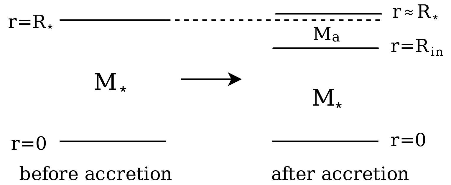
Although $R_{\textrm{in}}$ is treated as a hard surface for simplicity, it is not so in reality; a mountain several tens of meters high, whose base reaches neutron drip densities, sinks into the lower-density substrate (Wette et al. 2010; Priymak et al. 2011). A full treatment of sinking requires time-dependent simulations. Wette et al. 2010 showed that the results are approximated reasonably by hard-surface solutions (the mountain ellipticity decreases by a factor $\lesssim 2$ for soft crust solutions relative to hard-surface solutions), if $R_{\textrm{in}}$ corresponds to the layer above which the mass equals $M_{a}$; i.e. one has $R_{\textrm{in}}<R_{\star}$ and $M_{a}=\int^{r=R_{\star}}_{r=R_{\textrm{in}}}d^{3}\boldsymbol{x}\,\rho$. As $R_{\textrm{in}}$ is fixed, the stellar radius $R_{\star}$ varies slightly ($\leq 1$ per cent for $M_{a}\leq 10^{-4}M_{\odot}$) between models with different $M_{a}$ but the same EOS. Figure 2 visually demonstrates the relationship between $R_{\text{in}},R_{\star}$, and $M_{a}$.

Crustal matter experiencing compression due to accretion undergoes a variety of non-equilibrium nuclear processes, such as electron captures and beta decay, neutron emission and absorption, and pyconuclear fusion, all of which play a role in determining the EOS of the accreted crust (Sato 1979; Miralda-Escude et al. 1990; Chamel & Haensel 2008). The original outer crust, consisting of cold, catalysed matter, is replaced by a new, non-catalysed crust after $\lesssim 10^{5}\text{ yr}$ (Haensel & Zdunik 1990a). The EOS of an accreted, non-catalysed crust, relevant for our calculations, has been calculated numerically by Haensel & Zdunik 1990b by modeling the non-equilibrium processes listed above, using the compressible liquid drop model of Mackie & Baym 1977 to estimate the various thermodynamic rates which feed into the Gibbs equation [see also Sec. 2.4 of this paper and Bisnovatyĭ-Kogan & Chechetkin 1979].

In this paper we consider three idealized yet physically motivated polytropic EOS: a single-index model which best approximates (in a least-squares sense; see below) a realistic accreted crust (model A), and two of the classical ideal gas models considered by Priymak et al. 2011, corresponding to a gas of non-relativistic degenerate electrons (model B), and a gas of non-relativistic degenerate neutrons (model C). Their parameters are summarised in Table 1; see also Priymak et al. 2011. Models A, B, and C apply only at $t=0$; they are used to construct initial conditions for PLUTO. The Grad-Shafranov solver developed by Priymak et al. 2011 quasi-statically determines the ‘end-state’ of an adiabatic accretion process in the absence of thermal conduction. As noted above, we initialise PLUTO with an $M_{a}$-dependent Grad-Shafranov equilibrium to avoid numerical difficulties, cf. Wette et al. 2010. In reality, however, the true end-state of accretion depends on $\dot{M}_{a}$ as well as $M_{a}$. Accreted plasma on the stellar surface is expected to be approximately isothermal ($\Gamma\approx 1$) at all depths for low-accretion rates $\dot{M}_{a}\lesssim 10^{-10}M_{\odot}\text{ yr}^{-1}$ (Fujimoto et al. 1984; Zdunik et al. 1992). In contrast, a crust formed on a star accreting near the Eddington limit $\dot{M}_{a}\gtrsim 10^{-8}M_{\odot}\text{ yr}^{-1}$ has a more complicated polytropic EOS with a depth-dependent adiabatic index ($1\lesssim\Gamma\lesssim 5/3$) (Brown & Bildsten 1998; Brown 2000). Hence the time-dependent accretion process, which is not modeled here except implicitly through (9), directly affects the softness or hardness of the EOS. In particular, a self-consistent model of accretion along the lines of the sinking problem treated by Wette et al. 2010 would lead to end-state values of $k_{\Gamma}$ and $\Gamma$ which depend on both $M_{a}$ and $\dot{M}_{a}$ (Fujimoto et al. 1984; Brown et al. 1998). The numerical experiments we conduct in PLUTO, which evolve the EOS via thermal conduction, partially account for the effects of a near-Eddington accretion rate on the crustal EOS a posteriori (see Sec. 2.4). This procedure has been validated in the absence of thermal conduction by Wette et al. 2010.

In Figure 3 we graph pressure-density relationships for models A, B, and C (broken curves) together with the numerical results of Haensel & Zdunik 1990b (solid curve). For $\rho\gtrsim 1.5\times 10^{13}\text{ g cm}^{-3}$, the maximum density computed by Haensel & Zdunik 1990b, we graph the inner-crust model of Douchin & Haensel 2001, also computed using the compressible liquid drop model (Mackie & Baym 1977). Denoting the neutron drip density by $\rho_{\text{nd}}$ [$\rho_{\text{nd}}\sim 5\times 10^{11}\text{ g cm}^{-3}$ in an accreted crust (Chamel et al. 2015)], we see that the numerical results are approximated adequately by models B and C used in previous work (Priymak et al. 2011) in the regimes $\rho\ll\rho_{\text{nd}}$ and $\rho\gtrsim\rho_{\text{nd}}$ respectively. On the other hand, model A is constructed to uniformly approximate the realistic EOS for all $\rho\lesssim 10^{14}\text{ g cm}^{-3}$. The parameters $k_{\Gamma}$ and $\Gamma$ for model A are computed by fitting $p(\rho)=k_{\Gamma}\rho^{\Gamma}$ with the Levenberg-Marquardt (damped least-squares) algorithm (Press et al. 1986) to the data collated in Table 1 of Haensel & Zdunik 1990b. Denoting the Haensel & Zdunik 1990b numerical pressure by $p^{\text{HZ}}$ and the model A pressure by $p^{\text{A}}$, the fit yields relative errors of $0.94\leq p^{\text{HZ}}/p^{\text{A}}\leq 2.51$ for $10^{8}\leq\rho/\text{ g cm}^{-3}\leq 10^{14}$. Throughout most of the mountain volume by mass, i.e. for $\rho\geq 10^{12}\text{ g cm}^{-3}$, the errors drop to $\leq 6$ percent, with $0.95\leq p^{\text{HZ}}/p^{\text{A}}\leq 1.06$. For $\rho\leq 10^{9}\text{ g cm}^{-3}$ we have $0.94\leq p^{\text{HZ}}/p^{\text{A}}\leq 1.07$.

A piecewise polytropic fit to the solid curve in Fig. 3 (e.g. a spline fit to $\log p$ vs $\log\rho$) is a better approximation than the uniform, $\Gamma=1.18$ fit in model A. As a practical matter, however, it is difficult to generalise the Grad-Shafranov calculation in Sec. 2.2, especially the explicit formula for $F(\psi)$ [equation (8) in Priymak et al. 2011], to apply to multiple layers with proper matching at the inter-layer boundaries. As the Grad-Shafranov calculation is an essential input to the PLUTO simulations, the uniform $\Gamma=1.18$ approximation is the best we can do for now. For this reason, among others, the final results should be viewed as qualitatively representative models of the thermal conduction physics rather than quantitatively accurate mountain models to be compared in detail to observational data.

Different EOS predict different maximum (base) densities $\rho_{\text{max}}$ and heights $H$ for any given $M_{a}$. In Table 2 we list the characteristic $\rho_{\text{max}}$ and $H$ for runs performed in this paper (see Sec. 3.2) together with a rough estimate for the expected depth within a neutron star to which $\rho_{\text{max}}$ corresponds. Note that the sinking depths listed in Table 2 apply for stellar mass $M_{\star}=1.4M_{\odot}$, and a Skyrme-type EOS at zero temperature, used to describe both the crust and the liquid core, based on the effective nuclear interaction SLy (Douchin & Haensel 2001). Different EOS and stellar masses lead to different sinking depths. For models A and C, the theoretical depth exceeds the simulated height of the mountain. Depending on the crustal elasticity (Chamel & Haensel 2008), this indicates that mountain matter should sink beneath the surface and influence the hydromagnetic structure of the star (Konar & Choudhuri 2002). However, using breaking strain arguments, it has been shown that realistic crustal ellipticites of neutron stars cannot exceed $\sim 10^{-6}$ (Haskell et al. 2006; Johnson-McDaniel & Owen 2013), which is less than those associated with accreted mountains (see Sec. 4.2). As such, any gravitational radiation due to crustal quadrupole moment generation via back-reaction effects from a sinking mountain is likely to be dwarfed by the radiation due to the mountain itself (Wette et al. 2010), though there may be interesting consequences for other phenomena, e.g. crust-core coupling (Glampedakis & Andersson 2006). The lateral $(\theta)$ structure of the mountain is not affected greatly by sinking, as shown by Wette et al. 2010. Hence the main effect of sinking on $\epsilon$ is to reduce it by a factor $\approx\left(R_{\text{pre}}/R_{\text{post}}\right)^{5}$, where $R_{\text{pre}}$ and $R_{\text{post}}$ are the characteristic radii of the base of the mountain before and after sinking, respectively, and “before sinking” here means “in the context of a hard-surface Grad-Shafranov calculation”. In any case, because we do not model sinking, the values of the ellipticities (and heights) presented in this paper should be taken as upper limits. Modeling a realistic neutron star together with a sinking mountain in a way that simultaneously tracks the Alfvén and sinking time-scales is a difficult problem that will be considered in future work.

The steady-state solution to the Grad-Shafranov problem in section 2.2 serves as initial data for evolving the mountain dynamically. In the absence of viscosity and under the assumptions of infinite electric conductivity³³ 3 The Ohmic diffusion and thermal conduction time-scales (see Sec. 2.5) are in the ratio $\tau_{\text{d}}/\tau_{\textrm{c}}\approx 2\times 10^{-14}\left(\sigma/\text{ s}^{-1}\right)|\boldsymbol{B}|/|\boldsymbol{\nabla}^{2}\boldsymbol{B}|L^{-2}\left(\rho/10^{10}\text{ g cm}^{-3}\right)^{-1}$, for characteristic length-scale $L$ and electrical conductivity $\sigma$. In the crust-magnetosphere interface, one has $\sigma\lesssim 10^{16}\text{ s}^{-1}$ (Akgün et al. 2018). In the inner crust one has $\sigma\gtrsim 10^{24}\text{ s}^{-1}$ (Potekhin 1999; Potekhin et al. 2013). Hence we find $\tau_{\text{d}}/\tau_{\textrm{c}}\gg 1$ throughout the computational volume for the range of accreted masses considered in this paper, even in regions with strong magnetic gradients, because the density is low there $\left(\rho\lesssim 10^{10}\text{ g cm}^{-3}\right)$. We can therefore safely ignore the effects of Ohmic diffusion over the time-scales simulated within this paper; see also Vigelius & Melatos 2009c. (ideal MHD) and the Cowling approximation, the evolution is governed by the continuity, Euler, and Faraday equations, which read (Landau & Lifshitz 1959)

and

respectively, given $\phi$. The MHD equations (10)–(12) are closed by the energy equation,

where $T$ is the temperature, $\boldsymbol{F}$ is the heat flux, and $\varepsilon$ is the internal energy (Shapiro & Teukolsky 1983). The kinetic properties of the fluid determine the internal energy in terms of the thermodynamic variables $p,\rho$, and temperature $T$, i.e. $\varepsilon=\varepsilon(p,\rho,T)$ (Kundu & Cohen 2008). The Gibbs fundamental equation,

where $V$ is the system volume and $S$ is the entropy, provides an additional constraint for the state variables. We then have seven scalar equations, namely (10)–(14), for seven variables in the axisymmetric problem: $p,\rho,T,B_{r},B_{\theta},v_{r}$, and $v_{\theta}$. In practice, (15) determines $T$ given $p$ and $\rho$, while (2.4) determines the the relationship between $p$ and $\rho$, i.e. the barotropic EOS $p=p(\rho)$ initially. Under the assumption of an ideal gas (consistent with a polytropic EOS), equation (15) leads to the well-known relation (Shapiro & Teukolsky 1983)

where $\eta$ is the mean molecular weight, $m_{u}$ is the atomic mass unit and $k_{B}$ is the Boltzmann constant. The temperature field $T(p,\rho)$ in (16) is calculated from the Grad-Shafranov output and forms an additional input into PLUTO for thermal conduction simulations. We make the assumption of symmetric nuclear matter to determine $\eta$ for simplicity as in previous work [see section 2.3 of Priymak et al. 2011]. Although the ideal gas law (16) is modified in degenerate matter, it provides a good approximation for partially-degenerate, accreted material on a neutron star crust (Schatz et al. 1999) and is straightforward to handle within PLUTO. A sensitivity analysis associated with expression (16) is presented in Appendix B, where it is shown that using (16) to determine $T$ as opposed to a degenerate EOS calculated from first principles overestimates the temperature by $\lesssim 15\%$ throughout the bulk of the mountain (see also Secs. 2.3 and 3), where thermal transport matters most; a small effect compared to other uncertainties in the problem.

In the presence of thermal conduction, the flux on the left-hand side of (2.4) takes the form (Landau & Lifshitz 1959)

where the thermal conductivities $\kappa_{||}$ and $\kappa_{\perp}$, both measured in units of $\textrm{erg}\textrm{ s}^{-1}\textrm{ K}^{-1}\textrm{ cm}^{-1}$, describe heat transport parallel and perpendicular to the magnetic field respectively. The conductivities of a magnetised, fully ionized plasma are dominated by electron transport. They are given in the diffusion approximation by the Balescu-Braginskii formulas [see Braginskii 1965; Potekhin 1999 and Table 3.2 of Balescu 1988],

and

assuming the Coulomb logarithm satisfies $\ln\Lambda=30\approx\textrm{constant}$ (Balbus 1986). The estimates (18) and (19) are independent of the ideal gas assumption (16). In the limit of a vanishing magnetic field, one has $\kappa_{\perp}=\kappa_{||}$, and (17) reduces to $\boldsymbol{F}=\kappa_{||}\boldsymbol{\nabla}T$.

A mountain with the structure in Fig. 1 contains steep density and magnetic field gradients, so there is no unique definition for characteristic time-scales, like the Alfvén time $\tau_{\textrm{A}}$ and thermal conduction time $\tau_{\textrm{c}}$. In order to analyse our numerical results in Sec. 3 onwards, we adopt the definition (Mukherjee & Bhattacharya 2012)

where $L$ is taken to be the density scale-height where $\rho$ drops to $10^{-3}$ times its maximum value $\rho_{\text{max}}$, $\bar{\rho}$ is the volume-averaged density

where $V_{\textrm{m}}$ is the mountain volume ($10^{-7}\rho_{\text{max}}\leq\rho\leq\rho_{\text{max}}$) and $|\bar{\boldsymbol{B}}|$ is the volume-averaged magnetic field strength,

All the quantities (20)–(23) are computed at $t=0$ to define $\tau_{\textrm{A}}$ for any given run. Similarly, for thermal conduction, from the heat equation we have

where $\bar{\kappa}_{\perp}$, $\bar{\kappa}_{||}$, and $\bar{T}_{e}$ are volume-averaged quantities calculated in the same manner as $\bar{\rho}$ in (22) and $|\bar{\boldsymbol{B}}|$ in (23).

The thermal conduction time is $\sim 10^{6}$ times longer than the Alfvén time for a typical, realistic mountain. Computational expense restricts us to $t\lesssim 2\tau_{\textrm{c}}$ throughout most of this paper (see Sec. 3). The ratio of the time-scales varies from run to run and for different EOS. We perform some ‘long-term’ evolutions (up to $\sim 80\tau_{\textrm{c}}$) in Section 5 to explore the effects of thermal relaxation. In Sections 3 and 4 we show that (21) and (25) agree with the time-scales of characteristic behaviours observed empirically in the simulations.

We start by considering a representative simulation, which demonstrates the main features of thermal evolution: EOS model A with $M_{a}=1.8\times 10^{-5}M_{\odot}\approx 0.58M_{c}$. We set up a polytropic initial state ($\Gamma=1.18$ at $t=0$), allow thermal conduction to take place, and evolve the mountain. The EOS parameters, described in Table 1, are entered into the Grad-Shafranov solver, which produces the initial input for PLUTO. The thermal profile is entered according to (16). Two separate PLUTO instances are evolved, with and without the thermal flux $\boldsymbol{F}$ appearing in the right-hand side of equation (2.4). The time-scales (21) and (25) read $\tau_{\textrm{A}}\approx 2.0\times 10^{-5}\text{ s}$ and $\tau_{\textrm{c}}\approx 5.6\times 10^{6}\tau_{\textrm{A}}$.

In Figure 4, which demonstrates several features typical of an initially polytropic mountain, we graph contours of $\rho$ and magnetic field lines at $t=0$. The mountain reaches a maximum altitude of $H_{\text{max}}\approx 1.3\times 10^{3}\text{ cm}$ near $\theta=\pi/4$ (where $|\boldsymbol{B}|$ rises to a maximum). Most of the mass $(\approx 92\%)$ is concentrated within the octant $0\leq\theta\leq\pi/4$. The densest point, with $\rho=2.2\times 10^{13}\text{ g cm}^{-3}$, lies at the pole. The magnetic field lines are shifted equatorially; the maximum contour lies at $\theta=\pi/4$, in contrast to the initial dipole field (maximum at $\theta=0$).

Figure 5 presents results from PLUTO  and illustrates how thermal conduction affects the evolution. It shows snapshots at $t=2\tau_{\textrm{c}}$ of an adiabatic mountain ($\boldsymbol{F}=0$, left panel) and one evolved with a nonzero thermal flux ($\boldsymbol{F}\neq 0$, right panel). The mountain grows from $H_{\text{max}}\approx 1.3\times 10^{3}\text{ cm}$ to $H_{\text{max}}\approx 3.0\times 10^{3}\text{ cm}$. It is $\approx 4\%$ taller for the run with conduction, but its density is lower (by a factor $\lesssim 5$ near $\theta=0.1$ where an underdense column forms; see Sec. 3.2) everywhere except at $\theta\approx 0$ and $\theta\approx 0.2$. This is a consequence of the continuity equation (10), which demands that an increase in height is met with an overall decrease in mass density. Aside from the underdense column, thermal conduction has the effect of driving matter towards the pole, where the density attains a maximum of $\rho_{\text{max}}=1.3\times 10^{13}\text{ g cm}^{-3}$ for the run without conduction (left panel) and $\rho_{\text{max}}=1.5\times 10^{13}\text{ g cm}^{-3}$ for the run with conduction (right panel) ($\approx 16\%$ increase). An analogous thermal softening phenomenon occurs in crustquake models, where thermal transport amplifies shear stresses felt in the neutron star crust (Chugunov & Horowitz 2010; Beloborodov & Levin 2014).

Evolution with $\boldsymbol{F}\neq 0$ tends to widen the magnetic field contours (cf. Fig. 4), because the mountain spreads and drags the field-lines with it [the time-dependent version of the flux-freezing condition (8)]. Thermal conduction causes matter to be shifted both towards the pole and towards the base of the mountain, causing magnetic ‘pockets’ to form near $\theta=0$ (see also Sec. 3.2 and Fig. 6, where they are clearer), as the field lines bend around the drifting matter. Overall, the magnetic field is weakened, going from a maximum strength of $|\boldsymbol{B}|_{\text{max}}=2.9\times 10^{15}\text{ G}$ to $|\boldsymbol{B}|_{\text{max}}=1.9\times 10^{15}\text{ G}$ and $|\boldsymbol{B}|_{\text{max}}=2.0\times 10^{15}\text{ G}$ at $t=2\tau_{\textrm{c}}$ without and with conduction, respectively. Away from the pole, the locations of the maxima and minima of $|\boldsymbol{B}|$ are largely unaffected by conduction.

In Figure 6 we plot $\rho$ contours and magnetic field lines for model A (top row) with $M_{a}=2.4\times 10^{-5}M_{\odot}\approx 1.0M_{c}$, model B (middle row) with $M_{a}=3.0\times 10^{-8}M_{\odot}\approx 1.2M_{c}$, and model C (bottom row) with $M_{a}=2.0\times 10^{-6}M_{\odot}\approx 1.0M_{c}$ for times $t=0$ (left panel) and $t=2\tau_{\textrm{c}}$ without (middle panel) and with (right panel) thermal conduction. The initial state is read from the Grad-Shafranov output and is the same for both runs for any given EOS. All three runs have similar⁴⁴ 4 Ideally we would keep $M_{a}/M_{c}$ exactly the same across all runs. However, this is impractical because one does not know what $\mu$ is prior to running the Grad-Shafranov code for a given $M_{a}$, and it is computationally expensive to try and tune $M_{a}/M_{c}$ exactly. values of $M_{a}/M_{c}\sim 1$, implying that $\mu$ at $t=0$ is approximately halved by burial in all three models (see Sec. 4.1). We emphasise that models B and C are poor approximations to a realistic crust. They are included throughout mainly to give the reader a general sense of how the mountain structure depends on the EOS as well as to make contact with previous work for completeness.

The model A mountain (top row of Fig. 6) grows taller over time, thereby reducing $\bar{\rho}$; we find $H_{\text{max}}=3.3\times 10^{3}\text{ cm}$ for both $\boldsymbol{F}=0$ and $\boldsymbol{F}\neq 0$ at $t=2\tau_{\textrm{c}}$, compared to $H_{\text{max}}=1.2\times 10^{3}\text{ cm}$ at $t=0$. The magnetic pole remains the densest region with maximum densities $\rho_{\text{max}}=2.38\times 10^{13}\text{ g cm}^{-3}$ at $t=0$ and $\rho_{\text{max}}=1.43\times 10^{13}\text{ g cm}^{-3}$ at $t=2\tau_{\textrm{c}}$ without thermal conduction and $\rho_{\text{max}}=1.45\times 10^{13}\text{ g cm}^{-3}$ at $t=2\tau_{\textrm{c}}$ with thermal conduction. A narrow, underdense $(\rho\lesssim 4\times 10^{12}\text{ g cm}^{-3}$) column forms at $\theta\approx 0.1$ for the run with thermal conduction. Field lines are noticeably distorted from their $t=0$ state by flux freezing through a combination of poleward flow, which pushes them towards $\theta=0$, and stretching caused by the $\sim$ three-fold increase in $H_{\text{max}}$, which pushes them radially outward.

Equation (16) implies $\boldsymbol{\nabla}T\propto\boldsymbol{\nabla}\rho^{\Gamma-1}$. Hence we expect thermal conduction to be less influential in model A $(\Gamma=1.18)$ than in models B and C $(\Gamma=5/3)$. The evolution of adiabatic model B (middle row of Fig. 6) is noticeably affected by the non-zero flux term $\boldsymbol{F}$ (cf. middle and right panels). The matter column near the pole has height $H_{\text{max}}(\theta\approx 0)=1.8\times 10^{4}\text{ cm}$ for $\boldsymbol{F}=0$ and $H_{\text{max}}(\theta\approx 0)=3.0\times 10^{4}\text{ cm}$ for $\boldsymbol{F}\neq 0$. Matter concentrates more at the base of the mountain $(r\approx R_{\text{in}})$ for $\boldsymbol{F}\neq 0$, reaching peak densities of $\rho_{\text{max}}=6.8\times 10^{8}\text{ g cm}^{-3}$ for $\boldsymbol{F}=0$ and $\rho_{\text{max}}=9.2\times 10^{8}\text{ g cm}^{-3}$ for $\boldsymbol{F}\neq 0$ at $\theta=0$. Both evolved mountains are denser than the initial state $(\rho_{\text{max}}=6.4\times 10^{8}\text{ g cm}^{-3})$. Thermal conduction drives matter towards the pole, like what is seen in Fig. 5. The mountain grows taller, albeit comparatively less so than for model A, going from peak altitudes $H_{\text{max}}\approx 4.0\times 10^{4}\text{ cm}$ to $H_{\text{max}}\approx 4.2\times 10^{4}\text{ cm}$ with $\boldsymbol{F}=0$ and $H_{\text{max}}\approx 4.3\times 10^{4}\text{ cm}$ for $\boldsymbol{F}\neq 0$.

Adiabatic model C (bottom row of Fig. 6) evolves like model B. The mountain grows taller on the conduction time-scale, going from $H_{\text{max}}\approx 4.0\times 10^{3}\text{ cm}$ at $t=0$ to $H_{\text{max}}\approx 5.0\times 10^{3}\text{ cm}$ for $\boldsymbol{F}=0$ and $H_{\text{max}}\approx 5.3\times 10^{3}\text{ cm}$ for $\boldsymbol{F}\neq 0$. At $t=0$, the density maximum $\rho_{\text{max}}=3.7\times 10^{11}\text{ g cm}^{-3}$ lies at $r\approx R_{\text{in}}$ and $\theta=0$. After evolution the density reaches maximum values at the same location of $\rho_{\text{max}}=3.5\times 10^{11}\text{ g cm}^{-3}$ ($\approx 5\%$ decrease) for $\boldsymbol{F}=0$ and $\rho_{\text{max}}=4.0\times 10^{11}\text{ g cm}^{-3}$ ($\approx 8\%$ increase) for $\boldsymbol{F}\neq 0$ at $t=2\tau_{\textrm{c}}$. The compression of matter at the pole suggests that $\boldsymbol{F}\neq 0$ acts to ‘soften’ the effective EOS.

By inspecting the magnetic field lines in Fig. 6, we see that $|\boldsymbol{B}|$ evolves similarly to $\rho$ due to flux freezing. As discussed above, thermal conduction drives matter towards the pole, shifting $\boldsymbol{B}$ accordingly (Payne & Melatos 2004; Priymak et al. 2011). Hence $|\boldsymbol{B}|$ decreases on the whole as time passes, most dramatically in the case of model C, which predicts $|\boldsymbol{B}|_{\text{max}}=9.7\times 10^{14}\text{ G}$ at $t=0$, $|\boldsymbol{B}|_{\text{max}}=6.5\times 10^{14}\text{ G}$ for $\boldsymbol{F}=0$ at $t=2\tau_{\textrm{c}}$, and $|\boldsymbol{B}|_{\text{max}}=6.6\times 10^{14}\text{ G}$ for $\boldsymbol{F}\neq 0$. This is similar to what occurs for the representative example discussed in Sec. 3.1 and tests with different grid resolutions (not plotted), suggesting the possibility that $|\boldsymbol{B}|_{\text{max}}$ increases slightly for runs with conduction, independent of the EOS. Additional, higher-resolution convergence tests (cf. Appendix A) can be undertaken, if future observational applications warrant. The formation of dense filamentary regions $(\rho\sim 10^{-1}\rho_{\text{max}})$ for runs with $\boldsymbol{F}\neq 0$ at $\theta\approx 1.0$ causes several magnetic ‘pockets’ to form near the pole, as the magnetic field lines bend around poleward-drifting matter. The formation of filaments near the magnetic pole, as observed across all simulations with thermal conduction, may stem from thermal Parker-like instabilities (Parker 1953; Field 1965). These instabilities introduce ‘finger-like’ density structures, which emerge due to the propagation of contact discontinuities between lighter and denser sections of fluid (Stone & Gardiner 2007; Mouschovias et al. 2009). Although we only have one fluid in our model, the strong dependence of the conduction coefficient (19) on the local magnetic field strength, which varies strongly near the pole, may cause this ‘fenced-off’ behaviour. It has been shown that unstable modes grow faster in the presence of anisotropic thermal conduction (Lecoanet et al. 2012).

Figure 7 displays contours of temperature $T$ (colour scale) and the direction of the thermal flux $\boldsymbol{F}$ (arrows) extracted from the runs performed in Figure 6. We seek to identify the existence, and evolution, of thermal hot spots [e.g. Becker & Truemper 1997].

The temperature varies gradually with $r$ and $\theta$ for model A (top row), because the polytropic index $\Gamma$ is nearly unity. Nevertheless, the maximum (at the pole) and minimum (at the mountain-atmosphere interface) values of $T$ are in the ratio $T_{\text{max}}/T_{\text{min}}\approx 10$, a significant contrast. The thermal flux is predominantly directed towards the base of the mountain at all times, but becomes more ‘noisy’ at large $t$, when local hot spots form. At $t=2\tau_{\textrm{c}}$ we see that the temperature profile becomes more uniform away from the pole, suggesting that the model evolves towards an isothermal end state [$d/dt\left(p/\rho\right)\approx 0$ for $t\gg\tau_{\textrm{c}}$], even when thermal conduction is not implemented. At $\theta\approx 0.1$ for the run with $\boldsymbol{F}\neq 0$ (right panel) we see a region of relatively low temperature $(T_{\text{max}}/T\sim 6)$ form. This ‘heat sink’ is underdense as seen in Fig. 6, and is surrounded by the local hot spots $(T_{\text{spots}}\sim 5\times 10^{9}\text{ K})$ described above.

For Model B (middle row) we have $|\boldsymbol{F}|\approx 10^{23}\text{ erg}\text{ cm}^{-2}\text{s}^{-1}$, and $\boldsymbol{F}$ is predominantly directed towards the pole at $\theta=0$. In the run without conduction (middle panel) we see that $\boldsymbol{F}$ is almost indistinguishable from its $t=0$ counterpart except near the equator where heat flows into a hot column $(T\approx 6\times 10^{9}\text{ K})$ at $\theta=1.3$. The temperature evolves like the density, i.e. growing and spreading with $\rho$ (cf. Fig. 6). When conduction is switched on, a hot region ($T\gtrsim 8\times 10^{9}\text{ K}$) forms near the pole which extends to the mountain-atmosphere interface at $H_{\text{max}}\approx 4.2\times 10^{4}\text{ cm}$. The flux is highest at the mountain-atmosphere interface and at altitude $r-R_{\text{in}}\approx 1.3\times 10^{4}\text{ cm}$. The flux is directed in different directions throughout the column, suggesting that localised hot spots form in the densest part of the mountain. Away from the pole $(\theta\gtrsim 0.1)$, the heat flow is small $(|\boldsymbol{F}|\lesssim 10^{-2}|\boldsymbol{F}|_{\text{max}})$.

In Model C (right panel) at $t=0$, we see that heat flows towards the pole $(|\boldsymbol{F}|\approx 10^{21}\text{ erg}\text{ cm}^{-2}\text{s}^{-1})$ and away from the equator $(|\boldsymbol{F}|\approx 10^{20}\text{ erg}\text{ cm}^{-2}\text{s}^{-1})$. At $t=2\tau_{\textrm{c}}$, however, heat flows from the top of the mountain to the base near the equator $(\theta\approx 1.3)$, and little heat ($|\boldsymbol{F}|\lesssim 10^{-4}|\boldsymbol{F}|_{\text{max}}$) flows near the pole, where a hot column $(T\approx 8\times 10^{8}\text{ K})$ develops in a manner to similar to model B. Because of relation (16), the temperature profile evolves like the density and increases as the mountain grows $(T\propto\rho^{\Gamma-1}$); cf. Fig 6. Overall, the initially polytropic mountains respond similarly to thermal conduction by forming hot spots near the equator at $\theta\approx 1.3$ (models B and C) and near the pole at $\theta\approx 0.1$ (all models), where $|\boldsymbol{F}|$ is largest.

The theory of magnetic burial predicts that the global magnetic dipole moment for an axisymmetric mountain,

evaluated at $r\gtrsim R_{\text{m}}$, decreases as a function of $M_{a}$ (Brown & Bildsten 1998; Melatos & Phinney 2001). In order to explore the relationship between burial, accreted mass, and thermal conduction for different EOS, we calculate $\mu$ from for a variety of PLUTO simulations with thermal conduction switched on.

Figure 8 shows how $\mu$ (normalized to the pre-accretion value $\mu_{i}$) evolves due to thermal conduction for various accreted masses ($0.1\leq M_{a}/M_{c}\leq 1$; left to right) and initially adiabatic EOS ($1.18\leq\Gamma\leq 5/3$; top to bottom). Each panel displays $\mu(t)$ on a logarithmic temporal scale to capture both the MHD $(t\ll\tau_{\textrm{c}})$ and thermal $(t\gtrsim\tau_{\textrm{c}})$ dynamics. Again we emphasise that model A (top row of Fig. 8) corresponds most closely to an astrophysically realistic accreted crust. Models B and C are included for completeness to illustrate EOS-related trends and make contact with previous work (Priymak et al. 2011).

All the mountains depicted in Fig. 8 undergo an initially violent phase within $\lesssim 10^{2}\tau_{\textrm{A}}$, during which $\mu$ drops then rises. The behaviour observed in model A is similar to what is seen in Figures 6 and 14 of Vigelius & Melatos 2008 for example. It is largely driven by the MHD reconfiguration of the mountain rather than thermal conduction $(10^{2}\tau_{\textrm{A}}\ll\tau_{\textrm{c}})$ (Vigelius & Melatos 2008; Mukherjee et al. 2013a). We find that $\mu$ decreases slightly for all mountains (maximum of $\approx 7\%$ for model A with $M_{a}/M_{c}\approx 0.2$), independent of the EOS, from $t=0$ to $t\sim 10^{2}\tau_{\textrm{A}}$, consistent with previous ZEUS simulations (Payne & Melatos 2007). Note that the Grad-Shafranov equilibria, and hence the evolution, are insensitive to the exact value of the initial dipole moment $\mu_{i}$ provided that we have $M_{a}/M_{c}\lesssim 10$ [cf. the scaling law (1) introduced by Shibazaki et al. 1989] (Payne & Melatos 2004; Payne & Melatos 2007). In this context, insensitive means that $\mu/\mu_{i}$ depends on $\mu_{i}$ only through the ratio $M_{a}/M_{c}$ and not on $\mu_{i}$ in isolation. Since Priymak et al. 2011 found that $M_{c}\propto\mu_{i}^{2}$, the insensitivity condition $M_{a}/M_{c}\lesssim 10$ translates into an EOS-dependent lower bound for $\mu_{i}$. For the astrophysically relevant model A, we require [see expression (B26) of Priymak et al. 2011]

which is safely applicable to many LMXB systems, at least within the early stages of accretion (van den Heuvel & Bitzaraki 1995; Zhang & Kojima 2006). For $M_{a}/M_{c}\gtrsim 10$, the Grad-Shafranov modelling breaks down, and it is an open question whether the results are sensitive to $\mu_{i}$ or not.

On the longer time-scale $t\gtrsim\tau_{\textrm{c}}$, the behaviour of $\mu$ is qualitatively similar for all three initially polytropic EOS. In all cases, $\mu$ increases beyond $\mu_{i}$; runs with $M_{a}/M_{c}\gtrsim 0.1$ lead to $\mu(t\gtrsim\tau_{\textrm{c}})>\mu(t=0)$. In effect thermal conduction resurrects some of the buried field, e.g. $\mu$ increases by $\approx 14\%$ in the case of model C with $M_{a}/M_{c}\approx 0.2$. For runs with $M_{a}/M_{c}\gtrsim 0.5$, $\mu$ increases significantly from its initial value at $t=0$, e.g. by up to $\approx 80\%$ in the case of model B for $M_{a}=3.0\times 10^{-8}M_{\odot}\approx 1.2M_{c}$.

For a realistic accreted crust (model A), we find $0.64\leq\mu/\mu_{i}\leq 0.83$ for $0.2\leq M_{a}/M_{c}\leq 1$ at $t=2\tau_{\textrm{c}}$. Small changes in $\mu$ for $t\gtrsim\tau_{\textrm{c}}$ in model A suggest that conduction plays a comparatively minor role in the evolution of astrophysically realistic mountains. Nevertheless we find that substantial ($\mu/\mu_{i}\lesssim 0.5$) magnetic burial requires significantly greater accreted masses than previously estimated by Priymak et al. 2011; for example, $\mu(t=2\tau_{\textrm{c}})/\mu(t=0)=1.28$ for $M_{a}/M_{c}(t=0)\approx 1$ suggests an increase in the characteristic mass $M_{c}$ at $t=2\tau_{\textrm{c}}$ by a factor $\sim 2$.

The inclusion of thermal conduction has the effect of partially resurrecting the buried field by increasing $\mu$, which is similar to ‘softening’ the EOS [as found by Priymak et al. 2011]. The comparatively small increase in $\mu$ for model A (see Fig. 8) implies that the realistic EOS softens less than for models B and C. This is expected because the polytropic index $\Gamma=1.18$ is closer to unity (i.e. nearly isothermal), implying that $\boldsymbol{\nabla}T$ is smaller than for the isentropic gas models B and C.

The characteristic gravitational wave strain emitted by a continuous-wave source is (Thorne 1980; Brady et al. 1998)

where $I_{jk}$ is the moment-of-inertia tensor, $\nu$ is the spin frequency, $d$ is the distance from the Earth to the source, and $\epsilon$ is the mass ellipticity,

The magnitude of $\epsilon$ represents the primary uncertainty in estimating $h_{c}$ in practical astrophysics applications [see e.g. Aasi et al. 2014; Mastrano et al. 2015; Suvorov et al. 2016b; though cf. Suvorov 2018]. Here we can calculate $\epsilon$ directly from (29) using $\rho$ as output by PLUTO. Thus we can explore the effects of thermal conduction on the detectability of magnetic mountains using ground-based interferometers such as the Laser Interferometer Gravitational-Wave Observatory (LIGO) (Harry & LIGO Scientific Collaboration 2010; Haskell et al. 2015).

Figure 9 plots $\epsilon$ against time (in units of $\tau_{\textrm{c}}$) for different EOS and values of $M_{a}$. The layout is the same as in Fig. 8. All of the runs yield $\epsilon<0$, indicating that the star is prolate⁵⁵ 5 Since Vigelius & Melatos 2008 found that three-dimensional simulations of magnetic mountains relax to an almost axisymmetric state after a few Alfvén times (see Footnote 1), we expect the star to be prolate even without the assumption of axial symmetry.; the mountain is densest at the magnetic pole (Cutler 2002; Mastrano et al. 2011).

In contrast to the magnetic dipole moment (Sec. 4.1), $|\epsilon|$ increases with time for $t\gtrsim 10^{2}\tau_{\textrm{A}}$ for all runs with $M_{a}/M_{c}\gtrsim 0.1$, by up to $\approx 45\%$ in the astrophysically realistic model A with $M_{a}/M_{c}\approx 1$. We also find smaller but still significant increases in $|\epsilon|$ in models B $(\approx 30\%$ with $M_{a}/M_{c}\approx 1)$, and C $(\approx 27\%$ with $M_{a}/M_{c}\approx 1)$. This result is consistent with the leading-order behaviour of $\epsilon$ given by (2), which implies that $|\epsilon|$ increases with $M_{c}$ (Melatos & Payne 2005). As noted in Sec. 4.1, all runs display a $\gtrsim$ two-fold increase in $M_{c}$ at $t=2\tau_{\textrm{c}}$. Thermal conduction tends to facilitate the poleward drift of matter (see Sec. 3.2), thereby making the star more prolate.

References

- Aasi et al. (2014) Aasi, J., Abadie, J., Abbott, B. P., et al. 2014, ApJ, 785, 119
- Abbott et al. (2007) Abbott, B., Abbott, R., Adhikari, R., et al. 2007, Physical Review D, 76, 082001
- Akgün et al. (2018) Akgün, T., Cerdá-Durán, P., Miralles, J. A., & Pons, J. A. 2018, MNRAS, 481, 5331
- Alexiades et al. (1996) Alexiades, V., Amiez, G., & Gremaud, P. 1996, Com. Num. Meth. Eng., 12, 31
- Alfvén (1943) Alfvén, H. 1943, Arkiv for Astronomi, 29, 1
- Arons (1993) Arons, J. 1993, ApJ, 408, 160
- Arzoumanian et al. (2002) Arzoumanian, Z., Chernoff, D. F., & Cordes, J. M. 2002, ApJ, 568, 289
- Balbus (1986) Balbus, S. A. 1986, ApJ, 304, 787
- Balescu (1988) Balescu, R. 1988, Transport Processes in a Plasma (Amsterdam: North-Holland)
- Becker & Truemper (1997) Becker, W., & Truemper, J. 1997, A&A, 326, 682
- Beckers (1992) Beckers, J. M. 1992, SIAM Journal on Numerical Analysis, 29, 701
- Beloborodov & Levin (2014) Beloborodov, A. M., & Levin, Y. 2014, ApJL, 794, L24
- Bhattacharyya & Strohmayer (2006) Bhattacharyya, S., & Strohmayer, T. E. 2006, ApJL, 641, L53
- Bildsten (1998) Bildsten, L. 1998, ApJL, 501, L89
- Bisnovatyĭ-Kogan & Chechetkin (1979) Bisnovatyĭ-Kogan, G. S., & Chechetkin, V. M. 1979, Soviet Physics Uspekhi, 22, 89
- Blondin & Freese (1986) Blondin, J. M., & Freese, K. 1986, Nature, 323, 786
- Brady et al. (1998) Brady, P. R., Creighton, T., Cutler, C., & Schutz, B. F. 1998, Physical Review D, 57, 2101
- Braginskii (1965) Braginskii, S. I. 1965, Reviews of Plasma Physics, 1, 205
- Brown (2000) Brown, E. F. 2000, ApJ, 531, 988
- Brown & Bildsten (1998) Brown, E. F., & Bildsten, L. 1998, ApJ, 496, 915
- Brown et al. (1998) Brown, E. F., Bildsten, L., & Rutledge, R. E. 1998, ApJL, 504, L95
- Čada & Torrilhon (2009) Čada, M., & Torrilhon, M. 2009, Journal of Computational Physics, 228, 4118
- Cavecchi et al. (2017) Cavecchi, Y., Watts, A. L., & Galloway, D. K. 2017, ApJ, 851, 1
- Chakrabarty et al. (2003) Chakrabarty, D., Morgan, E. H., Muno, M. P., et al. 2003, Nature, 424, 42
- Chamel & Haensel (2008) Chamel, N., & Haensel, P. 2008, Living Reviews in Relativity, 11, 10
- Chamel et al. (2015) Chamel, N., Fantina, A. F., Zdunik, J. L., & Haensel, P. 2015, Physical Review C, 91, 055803
- Chandrasekhar (1956) Chandrasekhar, S. 1956, ApJ, 124, 232
- Chandrasekhar (1967) Chandrasekhar, S. 1967, New York: Dover, 1967,
- Chugunov & Horowitz (2010) Chugunov, A. I., & Horowitz, C. J. 2010, MNRAS, 407, L54
- Courant & Hilbert (1953) Courant, R., & Hilbert, D. 1953, Methods of Mathematical Physics, Vol. I (New York: Interscience Publication)
- Cumming (2004) Cumming, A. 2004, IAU Colloq. 190: Magnetic Cataclysmic Variables, 315, 58
- Cumming et al. (2001) Cumming, A., Zweibel, E., & Bildsten, L. 2001, ApJ, 557, 958
- Cutler (2002) Cutler, C. 2002, Physical Review D, 66, 084025
- Douchin & Haensel (2001) Douchin, F., & Haensel, P. 2001, A&A, 380, 151
- Faucher-Giguère & Kaspi (2006) Faucher-Giguère, C. A., & Kaspi, V. M. 2006, ApJ, 643, 332
- Field (1965) Field, G. B. 1965, ApJ, 142, 531
- Fujimoto et al. (1984) Fujimoto, M. Y., Hanawa, T., Iben, I., Jr., & Richardson, M. B. 1984, ApJ, 278, 813
- Galloway et al. (2008) Galloway, D. K., Muno, M. P., Hartman, J. M., Psaltis, D., & Chakrabarty, D. 2008, The Astrophysical Journal Supplement, 179, 360-422
- Galloway et al. (2014) Galloway, D. K., Premachandra, S., Steeghs, D., et al. 2014, ApJ, 781, 14
- Gardiner & Stone (2005) Gardiner, T. A., & Stone, J. M. 2005, Journal of Computational Physics, 205, 509
- Geppert & Viganò (2014) Geppert, U., & Viganò, D. 2014, MNRAS, 444, 3198
- Glampedakis & Andersson (2006) Glampedakis, K., & Andersson, N. 2006, Physical Review D, 74, 044040
- Goldreich & Reisenegger (1992) Goldreich, P., & Reisenegger, A. 1992, ApJ, 395, 250
- Harry & LIGO Scientific Collaboration (2010) Harry, G. M., & LIGO Scientific Collaboration 2010, Classical and Quantum Gravity, 27, 084006
- Haskell et al. (2006) Haskell, B., Jones, D. I., & Andersson, N. 2006, MNRAS, 373, 1423
- Haskell et al. (2015) Haskell, B., Priymak, M., Patruno, A., et al. 2015, MNRAS, 450, 2393
- Haensel & Zdunik (1990a) Haensel, P., & Zdunik, J. L. 1990, A&A, 227, 431
- Haensel & Zdunik (1990b) Haensel, P., & Zdunik, J. L. 1990, A&A, 229, 117
- van den Heuvel & Bitzaraki (1995) van den Heuvel, E. P. J., & Bitzaraki, O. 1995, A&A, 297, L41
- Johnson-McDaniel & Owen (2013) Johnson-McDaniel, N. K., & Owen, B. J. 2013, Physical Review D, 88, 044004
- Keek et al. (2010) Keek, L., Galloway, D. K., in’t Zand, J. J. M., & Heger, A. 2010, ApJ, 718, 292
- Klimchuk & Sturrock (1989) Klimchuk, J. A., & Sturrock, P. A. 1989, ApJ, 345, 1034
- Konar & Choudhuri (2002) Konar, S., & Choudhuri, A. R. 2002, Bulletin of the Astronomical Society of India, 30, 697
- Konar & Choudhuri (2004) Konar, S., & Choudhuri, A. R. 2004, MNRAS, 348, 661
- Konar (2010) Konar, S. 2010, MNRAS, 409, 259
- Kosiński & Hanasz (2006) Kosiński, R., & Hanasz, M. 2006, Astronomische Nachrichten, 327, 479
- Kundu & Cohen (2008) Kundu, P. K., & Cohen, I. M. 2008, Fluid Mechanics: Fourth Edition (London, England: Academic Press)
- Landau & Lifshitz (1959) Landau, L. D., & Lifshitz, E. M. 1959, Fluid Mechanics (Oxford: Pergamon Press)
- Lasky (2015) Lasky, P. D. 2015, PASA, 32, e034
- Lecoanet et al. (2012) Lecoanet, D., Parrish, I. J., & Quataert, E. 2012, MNRAS, 423, 1866
- Litwin et al. (2001) Litwin, C., Brown, E. F., & Rosner, R. 2001, ApJ, 553, 788
- Mackie & Baym (1977) Mackie, F. D., & Baym, G. 1977, Nuclear Physics A, 285, 332
- Mastrano et al. (2011) Mastrano, A., Melatos, A., Reisenegger, A., & Akgün, T. 2011, MNRAS, 417, 2288
- Mastrano & Melatos (2012) Mastrano, A., & Melatos, A. 2012, MNRAS, 421, 760
- Mastrano et al. (2015) Mastrano, A., Suvorov, A. G., & Melatos, A. 2015, MNRAS, 447, 3475
- Melatos & Payne (2005) Melatos, A., & Payne, D. J. B. 2005, ApJ, 623, 1044
- Melatos & Phinney (2001) Melatos, A., & Phinney, E. S. 2001, PASA, 18, 421
- Mignone et al. (2007) Mignone, A., Bodo, G., Massaglia, S., et al. 2007, The Astrophysical Journal Supplement, 170, 228
- Mignone & Tzeferacos (2010) Mignone, A., & Tzeferacos, P. 2010, Journal of Computational Physics, 229, 2117
- Miralda-Escude et al. (1990) Miralda-Escude, J., Paczynski, B., & Haensel, P. 1990, ApJ, 362, 572
- Misanovic et al. (2010) Misanovic, Z., Galloway, D. K., & Cooper, R. L. 2010, ApJ, 718, 947
- Miyoshi & Kusano (2005) Miyoshi, T., & Kusano, K. 2005, Journal of Computational Physics, 208, 315
- Mouschovias (1974) Mouschovias, T. C. 1974, ApJ, 192, 37
- Mouschovias et al. (2009) Mouschovias, T. C., Kunz, M. W., & Christie, D. A. 2009, MNRAS, 397, 14
- Mukherjee & Bhattacharya (2012) Mukherjee, D., & Bhattacharya, D. 2012, MNRAS, 420, 720
- Mukherjee et al. (2013a) Mukherjee, D., Bhattacharya, D., & Mignone, A. 2013, MNRAS, 430, 1976
- Mukherjee et al. (2013b) Mukherjee, D., Bhattacharya, D., & Mignone, A. 2013, MNRAS, 435, 718
- Narayan & Heyl (2003) Narayan, R., & Heyl, J. S. 2003, ApJ, 599, 419
- Nishimura (2005) Nishimura, O. 2005, Publications of the Astronomical Society of Japan, 57, 769
- Parker (1953) Parker, E. N. 1953, ApJ, 117, 431
- Patruno (2012) Patruno, A. 2012, ApJL, 753, L12
- Payne & Melatos (2004) Payne, D. J. B., & Melatos, A. 2004, MNRAS, 351, 569
- Payne & Melatos (2006a) Payne, D. J. B., & Melatos, A. 2006, ApJ, 641, 471
- Payne & Melatos (2006b) Payne, D. J. B., & Melatos, A. 2006, ApJ, 652, 597
- Payne & Melatos (2007) Payne, D. J. B., & Melatos, A. 2007, MNRAS, 376, 609
- Potekhin (1999) Potekhin, A. Y. 1999, A&A, 351, 787
- Potekhin et al. (2013) Potekhin, A. Y., Fantina, A. F., Chamel, N., Pearson, J. M., & Goriely, S. 2013, A&A, 560, A48
- Press et al. (1986) Press, W. H., Flannery, B. P., & Teukolsky, S. A. 1986, Cambridge: University Press, 1986,
- Priymak et al. (2014) Priymak, M., Melatos, A., & Lasky, P. D. 2014, MNRAS, 445, 2710
- Priymak et al. (2011) Priymak, M., Melatos, A., & Payne, D. J. B. 2011, MNRAS, 417, 2696
- Riles (2013) Riles, K. 2013, Progress in Particle and Nuclear Physics, 68, 1
- Sato (1979) Sato, K. 1979, Progress of Theoretical Physics, 62, 957
- Schatz et al. (1999) Schatz, H., Bildsten, L., Cumming, A., & Wiescher, M. 1999, ApJ, 524, 1014
- Shapiro & Teukolsky (1983) Shapiro, S. L., & Teukolsky, S. A. 1983, Black holes, white dwarfs, and neutron stars: The physics of compact objects (New York: Wiley-Interscience)
- Shibazaki et al. (1989) Shibazaki, N., Murakami, T., Shaham, J., & Nomoto, K. 1989, Nature, 342, 656
- Srinivasan et al. (1990) Srinivasan, G., Bhattacharya, D., Muslimov, A. G., & Tsygan, A. J. 1990, Current Science, 59, 31
- Stone & Gardiner (2007) Stone, J. M., & Gardiner, T. 2007, ApJ, 671, 1726
- Strohmayer & Bildsten (2003) Strohmayer, T., & Bildsten, L. 2006, Cambridge Astrophysics Series, 39, 113
- Suvorov et al. (2016a) Suvorov, A. G., Mastrano, A., & Melatos, A. 2016, MNRAS, 456, 731
- Suvorov et al. (2016b) Suvorov, A. G., Mastrano, A., & Geppert, U. 2016, MNRAS, 459, 3407
- Suvorov (2018) Suvorov, A. G. 2018, Physical Review D, 98, 084026
- Taam & van den Heuvel (1986) Taam, R. E., & van den Heuvel, E. P. J. 1986, ApJ, 305, 235
- Thorne (1980) Thorne, K. S. 1980, Reviews of Modern Physics, 52, 299
- Urpin & Geppert (1995) Urpin, V., & Geppert, U. 1995, MNRAS, 275, 1117
- Ushomirsky et al. (2000) Ushomirsky, G., Cutler, C., & Bildsten, L. 2000, MNRAS, 319, 902
- Vigelius & Melatos (2008) Vigelius, M., & Melatos, A. 2008, MNRAS, 386, 1294
- Vigelius & Melatos (2009a) Vigelius, M., & Melatos, A. 2009, MNRAS, 395, 1963
- Vigelius & Melatos (2009b) Vigelius, M., & Melatos, A. 2009, MNRAS, 395, 1985
- Vigelius & Melatos (2009c) Vigelius, M., & Melatos, A. 2009, MNRAS, 395, 1972
- Wang et al. (2012) Wang, J., Zhang, C. M., & Chang, H.-K. 2012, A&A, 540, A100
- Wette et al. (2010) Wette, K., Vigelius, M., & Melatos, A. 2010, MNRAS, 402, 1099
- Yoshida (2013) Yoshida, S. 2013, MNRAS, 435, 893
- Zdunik et al. (1992) Zdunik, J. L., Haensel, P., Paczynski, B., & Miralda-Escude, J. 1992, ApJ, 384, 129
- Zhang & Kojima (2006) Zhang, C. M., & Kojima, Y. 2006, MNRAS, 366, 137
Appendix A PLUTO simulations
Complete documentation for the PLUTO code was published by Mignone et al. 2007. The specific features we rely upon and optimize are discussed below.
Grid and time step
We employ a static, two-dimensional, polar grid with grid points. The radial grid comprises a logarithmic section with points for , and a uniform section with points for , where is defined arbitrarily at as the innermost radial grid point with . A mixed grid captures features with sharply different length-scales and minimizes the interpolation errors discussed in Sec. 3. We find that including additional grid points in the atmosphere () increases the computational cost without modifying perceptibly the observables computed in Sec. 4. The angular grid is uniformly spaced in over .
We employ a Runge-Kutta third-order time-stepper for safety, although we find by experimentation that the results are essentially indistinguishable from the second-order variant. We employ the third-order finite-volume spatial integrator ‘Lim03’ to interpolate between grid points (Čada & Torrilhon 2009). This scheme resolves local minima with high precision, e.g. strong gradients at the mountain-atmosphere interface. We use a time-step where is determined through equation (25). We print output files at various fractions of depending on the specifics of the run; cf. the horizontal-axes on Figs. 8 and 9. This is small enough to avoid Courant-Friedrichs-Lewy (CFL) instabilities for each run.
In order to avoid numerical instabilities we simulate the mountain together with an atmosphere which has a small but non-zero density taken as . The atmosphere alleviates numerical difficulties associated with strong gradients and prevents the density from dipping below zero due to numerical fluctuations. We find that varying in the range does not modify the observables discussed in Sec. 3 and 4 by more than . The code crashes for , because dips below zero somewhere unless we set , which is too expensive computationally. We define a flag that sets at every grid point after each time step so that the atmosphere has a minimum density of for all .
We find that the bilinear interpolation algorithm of PLUTO introduces errors of in the quantities calculated in Secs. 3 and 4 between the (grid-realigned) PLUTO output and the raw Grad-Shafranov data; cf. Figures 2 and 4 of Priymak et al. 2011 with Figs. 8 and 9.
Divergence cleaning and thermal conduction
Maxwell’s equations require at all times. Various strategies can be employed to minimise numerical deviations from . For example, the extended hyperbolic divergence cleaning algorithm (Mignone & Tzeferacos 2010) introduces Lagrange multipliers into Faraday’s law (12). Inspection of PLUTO output files confirms that vanishes to floating-point precision as a consequence of using this algorithm. The divergence cleaning algorithm is coupled with the approximate Riemann solver ‘hlld’ designed to resolve shocks and strong gradient phenomena (Miyoshi & Kusano 2005).
Thermal conduction (see Sec. 3) is implemented via the super-time-stepping algorithm available in PLUTO and described in Alexiades et al. 1996. The energy equation (2.4) has a parabolic Courant number associated with it, which depends on the value of the conduction coefficients and . Together with the usual Courant number condition (Landau & Lifshitz 1959), we require to avoid instabilities (Beckers 1992). Super-time-stepping allows for flux terms to be treated in a separate ‘super-step’ using operator splitting methods, so that need not be reduced to avoid parabolic CFL instabilities.
Implementation, stability, and convergence tests
We test our PLUTO simulations in four ways. For implementation: (i) We compute the total mass of the simulation at each time-step to check for mass leakage. (ii) We check the surface dipole moment and the velocity field to ensure that the boundary conditions described in Sec. 2.2 are implemented faithfully. For convergence: (iii) We vary the grid parameters and to check if the results depend on the spatial resolution (see Figs. 12 and 13). For stability: (iv) We vary the super-time-stepping parameters, the CFL parameters, and the thermal conduction coefficients (i.e. checking if the conduction and no-conduction runs match smoothly in the limit ). The convergence of the Grad-Shafranov code described in Sec. 2.2 is studied fully by Payne & Melatos 2004 and Priymak et al. 2011.
In Figures 12 and 13 we show the evolution of the ellipticity and dipole moment, respectively, for model B with and thermal conduction switched on, with grid points and varying values of (this parameter is introduced to artificially scale the conduction coefficients, see Sec. 5). Two major points are evident from these plots. First, the trends associated with increasing for model B are the same as was observed for model A in Sec. 5; and are monotonically increasing with increasing values of at , independent of the EOS and grid resolution. The second point concerns the convergence test (iii) detailed above: for the run (black, diamonds), all simulation parameters are identical to those for the simulations performed in Sec. 4 for the same accreted mass and EOS (middle figure of the middle panel), except that the resolution is lower for the runs presented here. Comparing the final ellipticity and values from Figs. 12 and 13 with those presented in Table 3 for the higher resolution run, we see only a small () disparity at late times, with , , , and .
Figure 14 plots the total mass as a function of time without (black, triangles) and with (blue, circles) thermal conduction for model B with . We see that, after an initial adjustment phase, the total mass returns to within () without (with) thermal conduction. This adjustment phase occurs for two separate reasons. The first is due to the artificial atmospheric density , introduced to ensure that the simulation does not produce at any point throughout the evolution. Some of this atmospheric mass actually gets pulled down into the mountain, after which the atmosphere resets, thus increasing the overall mass of the simulation slightly. Additionally, the Grad-Shafranov equilibria are defined over grids which are slightly different to those in PLUTO. Hence, at , the MHD equations are not exactly satisfied in PLUTO, leading to a temporary increase in the total mass. These two effects combine to increase the total mass in the initial stages of evolution. Table A2 in Payne & Melatos 2007 reports similar total mass changes during the adjustment phase. Figure 14 is typical for runs performed in this paper.
In Figure 15 we plot the surface dipole moment [equation (26) evaluated at ] as a function of time without (black, triangles) and with (blue, circles) thermal conduction for model A with . If the boundary conditions at the stellar surface [namely ] are implemented without numerical error, should keep its initial value . We see a slight variation (maximum of ). Figure 15 is typical for runs performed in this paper.
Appendix B Ideal-gas approximation to the equation of state
Strictly speaking, the accreted matter in the crust is partially degenerate (Schatz et al. 1999). In this appendix, we verify that it is reasonable to approximate the EOS by the ideal-gas formula (16), for ease of use in PLUTO, when calculating the perturbations to the mountain structure caused by thermal transport. The equilibrium configuration of the mountain before thermal transport is switched on is calculated for the full, degenerate, polytropic EOS (see Sec. 2).
In a Fermi-Dirac distribution, the mean occupancy for a single-particle orbital with energy is given by