A first search for a stochastic gravitational-wave background
from ultralight bosons
Abstract
Ultralight bosons with masses in the range can induce a superradiant instability around spinning black holes (BHs) with masses of order 10-100 . This instability leads to the formation of a rotating “bosonic cloud” around the BH, which can emit gravitational waves (GWs) in the frequency band probed by ground-based detectors. The superposition of GWs from all such systems can generate a stochastic gravitational-wave background (SGWB). In this work, we develop a Bayesian data analysis framework to study the SGWB from bosonic clouds using data from Advanced LIGO and Advanced Virgo, building on previous work by Brito et.al. Brito et al. 2017. We further improve this model by adding a BH population of binary merger remnants. To assess the performance of our pipeline, we quantify the range of boson masses that can be constrained by Advanced LIGO and Advanced Virgo measurements at design sensitivity. Furthermore, we explore our capability to distinguish an ultralight boson SGWB from a stochastic signal due to distant compact binary coalescences (CBC). Finally, we present results of a search for the SGWB from bosonic clouds using data from Advanced LIGO’s first observing run. We find no evidence of such a signal. Due to degeneracies between the boson mass and unknown astrophysical quantities such as the distribution of isolated BH spins, our analysis cannot robustly exclude the presence of a bosonic field at any mass. Nevertheless, we show that under optimistic assumptions about the BH formation rate and spin distribution, boson masses in the range are excluded at 95% credibility, although with less optimistic spin distributions, no masses can be excluded. The framework established here can be used to learn about the nature of fundamental bosonic fields with future gravitational wave observations.
Keywords:
gravitational waves, stochastic backgrounds, superradiant instability, Bayesian inferenceI Introduction
The first detection of gravitational waves (GWs) from binary black hole (BBH) Abbott et al. 2016a and neutron star (BNS) Abbott et al. 2017a coalescences by the Advanced Laser Interometer Gravitational-wave Observatory (LIGO) Aasi et al. 2015a and Advanced Virgo Acernese et al. 2015 represented a historical breakthrough, creating an alternative window through which to view the Universe. Furthermore, subsequent observations of BBH coalescence events have firmly established GW astronomy Abbott et al. 2016b; Abbott et al. 2017b; Abbott et al. 2017c; Abbott et al. 2017d; Abbott et al. 2018a, shedding new light on fundamental physics Abbott et al. 2016c and the nature of the stellar mass black hole (BH) population Abbott et al. 2016d; Abbott et al. 2018b. In the near future, Advanced LIGO and Advanced Virgo will be joined by additional detectors, like KAGRA Aso et al. 2013 and LIGO-India Iyer et al. 2011. A major target for the advanced detector network is the stochastic gravitational-wave background (SGWB), a superposition of many sources too faint to resolve individually Abbott et al. 2016e; Abbott et al. 2017e.
Ultralight bosons around spinning BHs have been proposed as a possible source of the SGWB Brito et al. 2017; Brito 2017. Superradiant instabilities induced by the bosonic fields co-rotating around BHs result in angular momentum extraction analogous to the so-called Penrose process Penrose 1969. This instability not only spins down the BH, but also triggers an exponential growth of the bosonic field. Subsequently the resulting bosonic cloud exhibits a time-dependent quadrupole moment, leading to GW radiation. We could obeserve these GWs with current ground-based GW detectors in two regimes – the “resolvable” regime in which nearby sources within can be directly detected Brito et al. 2017; Palomba et al. 2012; D’Antonio et al. 2018; Isi et al. 2018 and the “unresolvable” regime where a superposition of all other sources in the Universe will contribute to a SGWB Brito et al. 2017; Brito 2017.
Ground-based detectors are sensitive to bosons with a given mass scale that can be determined through dimensional-analysis Brito et al. 2017; Brito 2017. We expect a bosonic field with the mass to couple strongly to BHs whose Schwarzschild radius is comparable to the boson’s Compton wavelength , where is the reduced Planck constant and is the speed of light. For BHs of around , this implies
| (1) |
where is the gravitational constant and is the mass of a BH. In other words, only BHs within a relatively narrow window will significantly couple to bosonic field with a certain mass scale. This can be physically interpreted as follows. For a given boson mass, if BH mass is too large or small, the timescale of superradiant instability increases and its effect is exponentially suppressed Brito et al. 2017; Brito et al. 2015a; Dolan 2007. As we will demonstrate, Advanced LIGO could detect superradiant instabilities surrounding BHs, and therefore can probe boson masses near .
Light bosonic fields, such as QCD axions or axion-like particles have attracted attention, as a promising candidate of dark matter Arvanitaki 2010; Essig et al. 2013. It is challenging to use traditional particle physics experiments to probe the existence of light particles that do not couple strongly to ordinary matter, but we can use GW observations to study particle physics beyond the Standard Model Arvanitaki 2015; Arvanitaki 2017.
Since angular momentum extraction is followed by characteristic GW emission, the detection of this class of GWs could also provide an explanation for the possible abundance of low spin BHs Brito et al. 2015b, which is consistent with the current BH spin measurement by Advanced LIGO Abbott et al. 2016f; Abbott et al. 2017c; Abbott et al. 2017d; Abbott et al. 2018b. Additionally, the BH spin distribution is considered to be a crucial indicator of different BH formation channels Belczynski et al. 2016; Tutukov and YungelSon 1993; Sigurdsson and Hernquist 1993; Rodriguez et al. 2016. The discovery of ultralight bosons regulating BH spins would have significant implications for understanding BH formation scenarios.
Previous work has studied the SGWB from bosonic clouds Fan 2018; Brito 2017. Ref. Fan 2018 examined the detectability of a stochastic background from BHs spinning down, assuming the current ground-based detector network operates at design sensitivity. They assumed two different signal spectra, referred to as the Gaussian model and the quasi-normal-mode model, and using a Fisher analysis they also assessed the capability of extracting the component of their signal models from the total background including the CBC background. Ref. Brito 2017 computed the background spectrum expected from the superradiant instability assuming only an isolated BH population model. They also compared the predicted spectrum with the power-law integrated curves Thrane 2013 of Advanced LIGO to study its detectability. In this work, we will develop a Bayesian analysis framework to search for the SGWB from the superradiant instability and apply it to data from Advanced LIGO’s first observing run. We construct our signal model based on Brito et al. 2017; Brito 2017, additionally incorporating the expected contribution from remnant BHs produced by compact binary mergers to obtain a more accurate prediction.
This paper is structured as follows. In Section II we review the model of superradiant instabilities as previously computed in Brito et al. 2017; Brito 2017; Brito et al. 2015a. In Section III, we present the predicted SGWB signal, including the contribution from population of binary merger remnants. In Section IV, we present a Bayesian framework with which to search for this background. In Section V, we discuss the sensitive range in the boson mass and the model selection capability between this background and the projected SGWB that arises due to unresolved CBCs. Furthermore, in Section VI we show the range of excluded boson masses using data from Advanced LIGO’s first observing run. Finally, Section VII summarizes the results and future work.
In what follows, all quantities are described in units .
II Superradiant instability
Before describing the data analysis methods, first we briefly review the theoretical basis of the bosonic cloud model as described in Brito et al. 2017; Brito 2017. For a review of supperradiance, see Brito et al. 2015b. Hereafter, we will restrict ourselves to scalar (spin-0) fields. Although vector (spin-1) East 2017; Pani 2012; Baryakhtar et al. 2017 and tensor (spin-2) Brito 2013 fields can additionally induce superradiant instabilities, the scalar case has been investigated most extensively Arvanitaki 2015; Arvanitaki 2017; Dolan 2007; Yoshino and Kodama 2014; Brito et al. 2015b.
Incident radiation can by amplified by extracting energy and angular momentum from a BH. As a result, the mass and angular momentum of the BH transitions from the initial states to the final states , respectively. Denoting the frequency of the radiation by and letting be the quantum numbers for angular momentum, the condition for superradiance to occur is given by Brito et al. 2015b
| (2) |
where is the horizon angular velocity of the BH, given by
| (3) |
Here, is the dimensionless spin parameter and is the outer event horizon of a Kerr BH.
Using black hole perturbation theory, in the limit that the scalar field’s Compton wavelength is much larger than the radius of the BH (), where
| (4) |
an approximate expression can be found for the eigenfrequencies of the scalar field Dolan 2007; Brito et al. 2017:
| (5) | ||||
where are the quantum numbers for energy and angular momentum for a wave function in a spherical potential, is a positive numerical factor depending on , and are real quantities. The imaginary part of the eigenfrequency, , will be positive, indicating that the mode is (linearly) unstable, whenever Eq. (2) is satisfied11 1 Note that we have used the relation , which is valid to leading order in .. This instability leads to the formation of a scalar “cloud” around the BH. We define the instability timescale as the characteristic timescale over which the cloud forms. We will focus only on the , mode hereafter since this mode has the shortest timescale and dominates the gravitational-wave radiation. In the large Compton wavelength limit, the instability timescale is given by Brito 2017; Brito et al. 2015a; Brito et al. 2017
| (6) |

As illustrated in Figure 1, after the scalar cloud has been formed, the scalar field profile will source a stress-energy tensor with a time-dependent quadrupole moment. The energy stored in the rotating scalar field configuration will emit gravitational-waves, with a frequency of and a luminosity given by Brito 2017; Brito et al. 2015a; Brito et al. 2017
| (7) |
where is the total mass (energy) of the amplified scalar field configuration. Eventually, the scalar cloud will lose energy due to gravitational radiation. This process will happen over the course of the emission timescale , given by Brito 2017; Brito et al. 2015a; Brito et al. 2017
| (8) |
Crucially, there is a significant difference between the instability and emission timescales, . Thus, we make the approximation that the scalar cloud forms more or less instantaneously and then starts to emit GWs. Neglecting the emission of GWs during the growth of the scalar cloud, conservation of energy and angular momentum implies that Brito 2017
| (9) |
The amplification of the cloud stops when the condition is satisfied. Combining this with Eq. (9), we obtain the final mass of the BH
| (10) |
For the lowest mode , in the long Compton wavelength limit , the maximum mass of the scalar cloud reads
| (11) |
Thus, for typical parameters , about 10% of the energy of the initial BH is stored in the scalar cloud configuration.
Finally, we can evaluate the total GW energy emitted between the superradiance saturation and the present time as follows
| (12) |
where is the GW emission timescale. Here, the signal duration is reasonably defined as , in which is the age of the Universe . The SGWB will be calculated by summing the energy emitted by each source over the population of rotating BHs.
III Modeling the SGWB
Now we turn to modelling the SGWB produced by scalar clouds which form around BHs. We consider isolated BHs, following the model of Brito et al. 2017. We also derive the contribution due to remnant BHs formed from compact binary coalescences, and verify that it is smaller than the contribution of isolated BHs for most scalar masses of interest.
III.1 Framework to compute the SGWB
The SGWB is described by its energy density spectrum Allen and Romano 1999; Romano and Cornish 2017, defined as
| (13) |
where is the energy density of GWs existing in the Universe and is the critical energy density required to have a spatially flat Universe. The astrophysical SGWB has been studied for a wide array of sources Kowalska-Leszczynska et al. 2015; Rosado 2011; Marassi 2011; Wu 2012; Ölmez 2010; Jenkins and Sakellariadou 2018 and is generally given by
| (14) |
where is the source-frame energy spectrum of an individual astrophysical event, is the number of sources per unit comoving volume per unit source frame time, and is the multivariate probability distribution of the source parameters . Note that the source frame frequency is related to the observed frequency by a factor of the redshift: . The function is determined by standard cosmology
| (15) |
where and are the dimensionless matter density and the dimensionless cosmological constant density, respectively. We use the cosmological parameters inferred from Planck Ade et al. 2016, i.e. and .
When constructing a model for the SGWB from a superradiant instability, we take the source parameters to be BH masses and their dimensionless initial spin parameter . This represents the BH spin before spinning down due to the instability. We note that the GWs emitted from an individual system actually have a slight frequency drift caused by the change in the cloud’s binding energy during the GW emission Isi et al. 2018. However, its overall drift is well within the width of each frequency bin that we use for our analysis. This leads to the following simple spectrum for a single source
| (16) |
In order to compute the background due to unresolved sources, we only integrate over the range of parameters that produces a signal-to-noise ratio (SNR) of less than 8 in a typical search for the astrophysical system in question D’Antonio et al. 2018; Isi et al. 2018. Nevertheless, the specifics of this cutoff do not change the overall shape of the predicted spectra significantly.
III.2 BH population models
To search for and constrain the stochastic background from a superradiant instability, we will need to assume a specific source number density and the mass and spin distributions of BHs. Below, we will consider two possible BH populations: (i) isolated BHs formed by core-collapse supernovae (CCSNe) and (ii) BBH merger remnants.
III.2.1 Isolated black holes
Here we assume a population of isolated BHs born from CCSNe. Eq. (14) can be reorganized as
| (17) |
where is the source-frame BH formation rate per comoving volume per BH mass . For the probability density of , we assume a uniform distribution
| (18) |
where are the lower and upper limit of the distribution. Inspired by Brito 2017, we adopt two different parameterizations of , either (a) varying the lower limit and fixing , or (b) varying the upper limit and fixing . Note that the first case is more optimistic than the second case, as it ensures a population of high-spin BHs that readily yield superradiant instabilities. Although these models for admittedly quite simple, the true spin distribution of isolated BHs is extremely uncertain. As we will show, different values crucially affect the background spectrum.
The BH formation rate reads
| (19) | ||||
| (20) |
is the mass of the BH’s progenitor star, whose population properties follow the cosmic star formation rate (SFR) and initial mass function (IMF) . We adopt the SFR model proposed in Vangioni et al. 2015,
| (21) |
is the redshift at the progenitor’s time of birth, that is, , where is the lifetime of a progenitor based on Schaerer, D. 2002. Note that is the IMF defined in terms of stellar mass fraction. This implies that yields the ratio of the total mass of stars whose mass lies between to the whole stellar mass. Since the Salpeter IMF is chosen as in the mass range , its expression is22 2 One should not confuse it with the other definition, that is, the number fraction of stars whose mass lies between . Let this be . The Salpeter function in this definition follows .
| (22) |
The BH mass is related to the mass and metalliticity of the progenitor star via . In this work we use a numerical fit for given by Fryer et al. 2012. It follows that
| (23) |
Note that implicitly depends on redshift via the stellar metallicity , whose evolution over the cosmic history is evaluated in Ma et al. 2016. The lower BH mass cutoff of is set as .
III.2.2 Binary black hole merger remnants
We also consider remnant BHs formed by BBH mergers, whose background spectrum is evaluated such that
| (24) | ||||
represents a set of component masses of BBHs, i.e. the primary mass and the secondary mass ( by definition) and . is the BBH merger rate density for a given and . Unlike the spin distribution of isolated BHs, here can be motivated by both the spin measurement of final remnant BHs by Advanced LIGO and Virgo Abbott et al. 2016f; Abbott et al. 2017b; Abbott et al. 2017d; Abbott et al. 2017c and several numerical simulations for mergers of similar-mass BHs González 2007; Berti 2007; Rezzolla et al. 2008. Both suggest that the spin magnitude of final remnant BHs is around . Therefore, we assume all the remnant BHs initially have , namely
| (25) |
Following Abbott et al. 2017e; Abbott et al. 2017f; Abbott et al. 2016f, we adopt the BH mass distribution
| (26) |
with the constraints that and . We approximate the mass of remnant BHs as
| (27) |
where the binding energy of the inner most stable orbit in a binary system is subtracted from the total mass Maggiore 2007.
We evaluate the merger rate as described in Dominik et al. 2013; Abbott et al. 2016e; Abbott et al. 2017e; Abbott et al. 2017f,
| (28) |
where is the time delay between a binary formation and its merger and is the time delay distribution. is the redshift at the binary formation time , in which is the cosmic time at merger. Following Abbott et al. 2016e; Abbott et al. 2017e, we assume that: (i) the distribution is taken as in the range , where is Abbott et al. 2016e; Dominik et al. 2013 and is the Hubble time Nakar 2007; O’Shaughnessy et al. 2008; Dominik et al. 2012; Dominik et al. 2013, (ii) the formation rate of BBHs, both of which are lighter than , evolves proportionally to the SFR , (iii) the SFR of Vangioni et al. 2015 is consistent with the one used for the isolated BHs model (see Eq. (21)), (iv) massive binaries in which at least one of the two component masses is above cannot be formed in a high metallicity environment where ( is the solar metallicity). For the assumption (iv), we instead multiply the SFR by a weighting factor to account for the fraction of star formation in an environment where Madau and Dickinson 2014. In other words,
| (29) |
After marginalizing Eq. (28) over the component mass distribution , the calibration at is performed with the published estimate of local merger rate with the power-law mass distribution33 3 At the time of writing the paper, Advanced LIGO and Virgo collaboration published a new paper on the inferred BBH population property using their first and second observing runs and the local merger rate estimate has been updated. However, we stick to the local merger rate, previously estimated in Abbott et al. 2017b, to demonstrate the pipeline performance. The normalization with the new merger rate estimate will be considered in future work., Abbott et al. 2017b such that
| (30) |
Although we have assumed this rate is known exactly, we note that the true rate is uncertain – the current 90% credible bounds on the BBH merger rate span [9.7, 101]. This uncertainty will correspondingly introduce a systematic uncertainty in our prediction of the remnant spectrum , whose effect should be considered in future work.
III.3 Total background model
The actual background spectrum that one would observe is the sum of the contributions from these two BH populations, that is,
| (31) |
where the superscripts represent each of the isolated BH and BBH merger remnant population given by Eq. (17) and Eq. (24), respectively. For the comparison between these components, Fig. 2 shows background spectra computed from each BH population model, plotted with power-law integrated curves Thrane 2013 of Advanced LIGO at different phases and the CBC background approximated as a power-law spectrum Abbott et al. 2017e.
The solid curves are the energy density spectra contributed from the isolated BH population for different scalar masses under an assumption of a uniform distribution over . The spin distribution skewed towards high would simply scale the overall spectrum. See Fig. 2 of Brito 2017 for its dependence on different spin distributions. The dotted curves, meanwhile, show the contribution from BBH merger remnants. In general, the abundance of isolated BHs exceeds the merger rate by four orders of magnitude. The isolated BH channel therefore dominates the SGWB for scalar masses . However, if the , the SGWB from isolated BHs is significantly suppressed due to the lack of BHs heavier than . In other words, although scalar fields with is sensitively coupled to these heavy BHs (see Fig. 1 of Brito et al. 2017), such massive BHs are only rarely produced by CCSNe Fryer et al. 2012. In contrast, heavy BHs can readily be produced by the merger remnant channel, and so remnant BHs dominate the SGWB when .
It is worth noting that the SGWB may dominate the projected CBC background, which is approximated as
| (32) |
as inferred from Abbott et al. 2017e. We will discuss the capability to distinguish between these two signal models based on the Bayesian framework in Section V.4.

IV Search Method
This section provides the overview of a statistical methodology that can be used to claim a detection or to place constraints related to the model of the superradiant instability. Here, we assume the GW background to be; (a) isotropic, (b) unpolarized, (c) stationary and (d) Gaussian.
IV.1 Setup
The SGWB is analyzed by taking the cross-correlation between outputs from a pair of detectors. In this work we will focus on the case of two detectors for simplicity, but the formalism can be extended to handle a larger network of detectors Allen and Romano 1999; Romano and Cornish 2017. Following the notation of Callister et al. 2017, we define a cross-correlation estimator for each frequency bin Aasi et al. 2015b; Romano and Cornish 2017 as,
| (33) |
Here, is the Fourier transform of time series output of the -th detector and is the total observation time. This is normalized such that
| (34) |
where is the overlap reduction function to encode the geometry and separation between a pair of detectors Flanagan 1993. In the low signal-to-noise limit, the variance is approximately given by
| (35) |
where is frequency resolution and is the power spectral density (PSD) of the -th detector.
Then, the unbiased broadband estimator and its variance can be constructed from and as follows
| (36) |
and
| (37) |
where is a linear filter formed by a given background model , so that
| (38) |
Once the broadband estimator is obtained, the SNR can be computed in a straightforward manner.
| (39) |
IV.2 Bayesian inference
We now develop a Bayesian formalism to perform parameter estimation and model selection for the superradiant instability model, following Mandic et al. 2012. In practice, the GW signal can be described by a set of unknown parameters and one needs to evaluate their posterior probability given new data. Then, Bayes’ theorem states that
| (40) |
where is the cross-correlation estimator over frequency band computed from observed data and is a set of parameters characteristic of GW signals in the signal hypothesis . is the posterior probability on the multi-dimensional space, is the likelihood, is the prior probability and is the evidence. To construct a posterior in an efficient manner, we apply the PyMultiNest package Buchner, J. et al. 2014 to our search pipeline. PyMultiNest is a python interface to the nested sampling package MultiNest Feroz and Hobson 2008; Feroz et al. 2009; Feroz et al. 2013, which produces a set of samples drawn from an estimated posterior.
IV.2.1 Likelihood
For one realization of , the joint likelihood over frequency bins is given by Mandic et al. 2012
| (41) |
is the likelihood within a single frequency bin. We assume a Gaussian likelihood, such that
| (42) | ||||
Here, is a model energy-density spectrum for a given set of parameters .
IV.2.2 Posterior
We choose a uniform prior on every parameter (e.g. scalar mass and spin limits ):
| (43) |
Our posteriors are therefore proportional to the likelihood:
| (44) |
We will often consider the marginalized posterior for a particular parameter, , which is defined as
| (45) |
The marginalized posterior will allow us to define credible intervals for the parameter in a standard way.
IV.2.3 Model selection
In order to perform model selection between different models of the SGWB, we need to compute the Bayesian evidence for each hypothesis. Let be the cross-correlation estimator obtained from the data and suppose that one assesses which model, or , is better supported by the data. It is straightforward to compute the odds ratio , which is defined as
| (46) |
where and are the evidences for each model. The evidence is calculated through
| (47) |
This expression can also be interpreted as the fully-marginalized likelihood. In the case where no signal is present (the null hypothesis ), the evidence is obtained by fixing to zero. Also in Eq. (46) is the so-called Bayes factor, while is a priori probability ratio for the two models, which we will set as unity. Since in our framework the odds ratio Eq. (46) is effectively equivalent to the Bayes factor, hereafter we will evaluate statistical significance in terms of the Bayes factor and follow the convention that a log Bayes factor of indicates a favor for a model over the other with great confidence Jeffreys 1961.
V Results
In this section, we first describe the parameterization of our signal model. Section V.2 shows a scheme for injecting simulated signals into Gaussian noise and recovering those signals. We then discuss the implications of performed analysis tests, including the construction of a “sensitivity window” of scalar masses to which Advanced LIGO might be sensitive. In Section V.4, we examine prospects for successfully discriminating between a CBC background and a SGWB due to supperradiant instability.
V.1 Parameters for the background model
In this work, the signal model is parameterized by the scalar mass and either or (refer to Sections III.2.1 for the details). We note that this model contains several sources of systematic uncertainty, such as the BH formation and merger rates as well as the underlying SFR. Nevertheless, we will assume a particular SFR (Eq. (21)) and binary formation rate (Eq. (30)). Our results are also conditional on our specific parameterization of the . A different choice for the BH spin distribution will generically yield different constraints on . Also, posteriors will be constructed over the two-dimensional parameter space of and either or .
V.2 Injection scheme and signal recovery
Here we describe the overview of the injection scheme adopted in this work. We assume only the LIGO detector pair, that is, the Hanford and Livingston sites. Injections are performed in the frequency domain. Given a PSD of the LIGO detectors, one constructs the variance of a cross-correlation estimator given by Eq. (35). A cross-correlation spectrum consistent with Gaussian noise is then constructed from this variance and the SGWB predicted from superradiant instability is added to the Gaussian noise. Therefore, the simulated cross-correlation spectrum is defined as
| (48) |
where is the overlap reduction function for the LIGO baseline Flanagan 1993, is the injected background constructed from the parameters , and is a random variable drawn from a Gaussian distribution with zero mean and unit variance. From this simulated cross-correlation spectrum, our pipeline infers the parameters by computing the likelihood and constructing a Bayesian posterior. We adopt a uniform prior for across the range and a uniform prior for or between 0 and 1.


Fig. 3 shows an example cross-correlation spectrum as a function of frequency using two years of observation with Advanced LIGO’s design sensitivity. The red dashed line gives the injected signal. The injection has SNR 32 and corresponds to the superradiant instability model with and . The magenta region represents the model evaluated with 100 sets of the parameters randomly drawn from the posterior. Fig. 4 shows the resulting posterior on and derived from this simulated observation. These figures both demonstrate that the pipeline can recover a loud injection with great confidence. A statistical discussion for a consistency test of the parameter estimation is described in Appendix A.
V.3 Sensitivity window
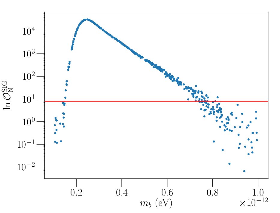
To study the scalar mass space we can probe through this model, which we refer to as the “sensitivity window”, we make a number of injections and compute their Bayes factors between the signal and noise hypotheses. The signal injection is performed in the same way as Eq. (48). For this test, we conservatively adopt the parameterization and the injected value is fixed as . The value for each of the 500 injections is uniformly drawn from the range . In Fig. 5, we recognize the injections above a log Bayes factor of 8 as detectable. Therefore, the range in which a log Bayes factor is larger than 8 (presented as the red line in Fig. 5) can be interpreted as the sensitivity window, which is around in Fig. 5. Note that the actual sensitivity window depends on spin parameter . Since larger simply scales the overall spectrum by a constant factor, we can have a wider detectable range of scalar masses for a larger .
V.4 Distinguishing superradiant instability and CBC backgrounds
As seen in Fig. 2, the SGWB signal from the superradiant instability model dominates over the projected CBC background for some choices of scalar mass and BH spins. Thus, the next question to address is “Given a detected signal, can we distinguish these two models from one another?” Here, we consider the case where both the superradiant instability and the projected CBC background are present, so that
| (49) |
where is the background due to superradiant instabilities under the parametrization given by Eq. (31), and is the fixed CBC background approximated as the power law spectrum shown in Eq. (32). Note that, after three years of observation with Advanced LIGO’s design sensitivity, alone is detectable with a log Bayes factor of 8.8 between a CBC-only and a noise model, which corresponds to an SNR of 5.5.
Given a simulated measurement of the combined background shown in Eq. (49), we recover our measurements with different two models: a CBC-only model and a joint superradiant instabiltity and CBC model (SICBC). The CBC background model for recovery is parameterized by a power-law index and an amplitude at the reference frequency , such that
| (50) |
We refer to Eq. (50) as a CBC model, even though this could be generally called “power-law spectrum model”, because the degrees of freedom in this model can be used to recover the parameters of the CBC injection. Also, priors for and are taken as a uniform distribution in the range of and respectively, while the priors for and are identical to those described in Section V.2. The parameters considered when evaluating the evidence for each background model are listed in Table 1.

We compute a log Bayes factor between these two hypotheses. The computation is repeated, changing injected values until we explore a grid over the entire prior space. Thus, we can probe the parameter space on which the superradiant instability signal can be discerned from the expected CBC background with statistical significance. Fig. 6 is a gray-scale map of a log Bayes factor, effectively equivalent to Eq. (46), with two contours of (magenta) and (cyan). Since the injected CBC background is loud enough to be detected in this simulation, Fig. 6 implies that inside the magenta contour one can expect the superradiant instability background to be distinguished from the CBC’s.
| Models | CBC | SICBC |
|---|---|---|
| Parameters |
VI Application to the first observing run of Advanced LIGO


We now apply our method to the cross-correlation spectrum measured in Advanced LIGO’s first observing run Abbott et al. 2017f (the data products given in that paper are publicly available at LIGO-G1602446). No statistically significant signal is detected, so we attempt to exclude some of the two-dimensional space of and through the search. Figs. 7 and 8 show the posteriors obtained under the and parametrizations, respectively. Fig. 7 indicates that, for the case, the posterior is almost uniformly distributed. Thus, no significant constraint can currently be placed on when is allowed to vary. This can be also verified by the fact that, according to Fig. 2, almost none of the possible spectra with the parameterization can reach the O1 power-law integrated curve. On the other hand, if we fix and allow the lower bound to vary, then Fig. 8 suggests that the mass range is excluded. This can be understood by Fig. 2 as well, which shows the largest SGWB amplitude when . As a forecast for the future, Appendix B shows the constraints that will be possible once Advanced LIGO reaches its design sensitivity.
VII Conclusion
This paper presents a first search for signs of supperradiant instability in the SGWB. We describe several performance tests of our search pipeline in Section IV. First, a detectable window in scalar mass is estimated from a Bayes factor of injections as shown in Fig. 5. Second, we study the capability to distinguish the model presented here from the fiducial CBC background model. The gray-scale map of log Bayes factors suggests that it is separable from the CBC model with statistical significance in some parameter space (see Fig. 6).
Finally, we present results obtained by analyzing data from Advanced LIGO’s first observing run. No signal is detected with either of our parameterizations of the BH spin distribution, and so we present constraints on possible boson masses and BH spin bounds. Using the parametrization, we cannot place any meaningful constraints on the scalar mass, while the case rules out the scalar mass range with 95% percent credibility. Let us note that this constraint is still subject to our choice of the BH spin distribution as well as specific astrophysical models we adopt in this work.
Future work will generalize the model to take into account effects of astrophysical uncertainties such as BH formation rate and the initial spin distribution for BBH remnant BHs. Also, the updated local merger rate Abbott et al. 2018b should be revisited. As the sensitivity increases with future observing runs of Advanced LIGO and Advanced Virgo, this framework can be used to place stronger constraints on the existence of ultralight bosons.
Acknowledgements.
We thank Richard Brito and Irina Dvorkin for their fruitful discussion and comments. L.T is supported by JSPS KAKENHI Grant Number JP18J21709. LIGO was constructed by the California Institute of Technology and Massachusetts Institute of Technology with funding from the National Science Foundation and operates under cooperative agreement PHY-0757058. A.M and P.M are supported by NSF grant PHY1505870. Parts of this research were conducted by the Australian Research Council Centre of Excellence for Gravitational Wave Discovery (OzGrav), through project number CE170100004. This paper carries LIGO Document Number LIGO-P1800232.Appendix A Consistency test of the parameter estimation
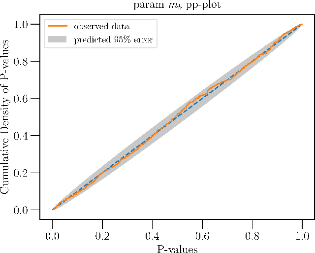
As a statistical consistency check of the parameter estimation performed by our pipeline using PyMultiNest, we construct a probability-probability plot (p-p plot) by performing 500 injections into simulated Gaussian noise drawn from the observed spectrum from Advanced LIGO’s O1 run. For each injection, we first construct the marginalized posterior for . We then compute the percentile (or p-value), which is defined by
| (51) |
where denotes the label of a given injection, the marginalized posterior for , the injected value and the lower limit of the prior space. We then plot the fraction of injections with -values less then a given threshold , as a function of the threshold. For correctly constructed posteriors we expect that for a given threshold , the fraction of injections with p-values smaller than the threshold is . If this is the case, then the injections will form a straight line with unit slope on the pp-plot. Fig. 9 shows the pp-plot we obtain with our injection campaign. The gray shadow is the credible error region predicted by statistical fluctuations from the ideal diagonal. Since the orange curve obtained by data lies within the error region, the pipeline consistently reproduces the parameters regardless of the loudness of those injections.
Appendix B Demonstration of possible constraints on scalar mass at the design sensitivity
We run the pipeline with synthesized noise data to demonstrate constraints on scalar mass expected from null result by three years of observation with the Advanced LIGO’s design sensitivity. Following the definition Eq. (33) and Eq. (35), the cross-correlation estimator and its variance for individual frequency bins are computed.


Figs. 10 and 11 each shows a two-dimensional posterior with different parameterizations. When is left free, the posterior excludes all scalar masses above , as shown in Fig. 10. In Fig. 11, on the other hand, more stringent constraints are placed in lighter scalar mass and the constraints become looser in the heavier boson mass regime. This is due to the strong dependence of the GW background amplitude on . More interestingly, the projected design sensitivity would place quite different constraints depending on the parameterization. While parameterization excludes upper part of prior space, , the parameterization could exclude the lower edge.
References
- Brito et al. (2017) R. Brito et al., Physical Review D 96 (2017), 10.1103/PhysRevD.96.064050.
- Abbott et al. (2016a) B. P. Abbott et al., Physical Review Letters 116 (2016a), 10.1103/PhysRevLett.116.061102.
- Abbott et al. (2017a) B. P. Abbott et al., Physical Review Letters 119 (2017a), 10.1103/PhysRevLett.119.161101.
- Aasi et al. (2015a) J. Aasi et al. (LIGO Scientific), Class. Quant. Grav. 32, 074001 (2015a), arXiv:1411.4547 [gr-qc] .
- Acernese et al. (2015) F. Acernese et al. (VIRGO), Class. Quant. Grav. 32, 024001 (2015), arXiv:1408.3978 [gr-qc] .
- Abbott et al. (2016b) B. P. Abbott et al., Physical Review Letters 116 (2016b), 10.1103/PhysRevLett.116.241103.
- Abbott et al. (2017b) B. P. Abbott et al., Physical Review Letters 118 (2017b), 10.1103/PhysRevLett.118.221101.
- Abbott et al. (2017c) B. P. Abbott et al., Physical Review Letters 119 (2017c), 10.1103/PhysRevLett.119.141101.
- Abbott et al. (2017d) B. P. Abbott et al., (2017d), 1711.05578 .
- Abbott et al. (2018a) B. P. Abbott et al., LIGO-P1800307 (2018a), 1811.12907 .
- Abbott et al. (2016c) B. P. Abbott et al. (Virgo, LIGO Scientific), Phys. Rev. Lett. 116, 221101 (2016c), [Erratum: Phys. Rev. Lett.121,no.12,129902(2018)], arXiv:1602.03841 [gr-qc] .
- Abbott et al. (2016d) B. P. Abbott et al. (Virgo, LIGO Scientific), Astrophys. J. 818, L22 (2016d), arXiv:1602.03846 [astro-ph.HE] .
- Abbott et al. (2018b) B. P. Abbott et al., (2018b), 1811.12940 .
- Aso et al. (2013) Y. Aso et al. (The KAGRA Collaboration), Phys. Rev. D 88, 043007 (2013).
- Iyer et al. (2011) B. Iyer et al., https://dcc.ligo.org/LIGO-M1100296/public (2011).
- Abbott et al. (2016e) B. P. Abbott et al., Physical Review Letters 116 (2016e), 10.1103/PhysRevLett.116.131102.
- Abbott et al. (2017e) B. P. Abbott et al., (2017e), 1710.05837 .
- Brito (2017) R. Brito, Physical Review Letters 119 (2017), 10.1103/PhysRevLett.119.131101.
- Penrose (1969) R. Penrose, Nuovo Cimento Rivista Serie 1 (1969).
- Palomba et al. (2012) C. Palomba, L. S. Collaboration, and V. Collaboration, (2012), 1201.3176 .
- D’Antonio et al. (2018) S. D’Antonio et al., LIGO-P1800247 (2018).
- Isi et al. (2018) M. Isi, L. Sun, et al., LIGO–P1800270 (2018).
- Brito et al. (2015a) R. Brito, V. Cardoso, and P. Pani, Classical and Quantum Gravity 32, 134001 (2015a).
- Dolan (2007) S. R. Dolan, Physical Review D 76 (2007), 10.1103/PhysRevD.76.084001.
- Arvanitaki (2010) A. Arvanitaki, Physical Review D 81 (2010), 10.1103/PhysRevD.81.123530.
- Essig et al. (2013) R. Essig et al., (2013), 1311.0029 .
- Arvanitaki (2015) A. Arvanitaki, Physical Review D 91 (2015), 10.1103/PhysRevD.91.084011.
- Arvanitaki (2017) A. Arvanitaki, Physical Review D 95 (2017), 10.1103/PhysRevD.95.043001.
- Brito et al. (2015b) R. Brito, V. Cardoso, and P. Pani, (2015b), 1501.06570 .
- Abbott et al. (2016f) B. P. Abbott et al., Phys. Rev. X 6, 041015 (2016f).
- Belczynski et al. (2016) K. Belczynski, D. E. Holz, T. Bulik, and R. O’Shaughnessy, Nature 534, 512 EP (2016).
- Tutukov and YungelSon (1993) A. V. Tutukov and L. R. YungelSon, Monthly Notices of the Royal Astronomical Society 260, 675 (x1993).
- Sigurdsson and Hernquist (1993) S. Sigurdsson and L. Hernquist, Nature 364, 423 EP (1993).
- Rodriguez et al. (2016) C. L. Rodriguez, M. Zevin, C. Pankow, V. Kalogera, and F. A. Rasio, The Astrophysical Journal Letters 832, L2 (2016).
- Fan (2018) X.-L. Fan, Physical Review D 98 (2018), 10.1103/PhysRevD.98.044020.
- Thrane (2013) E. Thrane, Physical Review D 88 (2013), 10.1103/PhysRevD.88.124032.
- East (2017) W. E. East, Physical Review Letters 119 (2017), 10.1103/PhysRevLett.119.041101.
- Pani (2012) P. Pani, Physical Review D 86 (2012), 10.1103/PhysRevD.86.104017.
- Baryakhtar et al. (2017) M. Baryakhtar, R. Lasenby, and M. Teo, (2017), 1704.05081 .
- Brito (2013) R. Brito, Physical Review D 88 (2013), 10.1103/PhysRevD.88.023514.
- Yoshino and Kodama (2014) H. Yoshino and H. Kodama, Progress of Theoretical and Experimental Physics 2014, 043E02 (2014).
- Allen and Romano (1999) B. Allen and J. D. Romano, Phys. Rev. D 59, 102001 (1999).
- Romano and Cornish (2017) J. D. Romano and N. J. Cornish, Living Reviews in Relativity 20, 2 (2017).
- Kowalska-Leszczynska et al. (2015) I. Kowalska-Leszczynska, T. Regimbau, et al., A&A 574, A58 (2015).
- Rosado (2011) P. A. Rosado, Physical Review D 84 (2011), 10.1103/PhysRevD.84.084004.
- Marassi (2011) S. Marassi, Physical Review D 84 (2011), 10.1103/PhysRevD.84.124037.
- Wu (2012) C. Wu, Physical Review D 85 (2012), 10.1103/PhysRevD.85.104024.
- Ölmez (2010) S. Ölmez, Physical Review D 81 (2010), 10.1103/PhysRevD.81.104028.
- Jenkins and Sakellariadou (2018) A. Jenkins and M. Sakellariadou, (2018), 1802.06046 .
- Ade et al. (2016) P. A. R. Ade et al., A&A 594, A13 (2016).
- Vangioni et al. (2015) E. Vangioni, K. A. Olive, T. Prestegard, J. Silk, P. Petitjean, and V. Mandic, Monthly Notices of the Royal Astronomical Society 447, 2575 (2015).
- Schaerer, D. (2002) Schaerer, D., A&A 382, 28 (2002).
- Fryer et al. (2012) C. L. Fryer, K. Belczynski, G. Wiktorowicz, M. Dominik, V. Kalogera, and D. E. Holz, The Astrophysical Journal 749, 91 (2012).
- Ma et al. (2016) X. Ma, P. F. Hopkins, C.-A. Faucher-Giguère, N. Zolman, A. L. Muratov, D. Kereš, and E. Quataert, Monthly Notices of the Royal Astronomical Society 456, 2140 (2016).
- González (2007) J. A. González, Physical Review Letters 98 (2007), 10.1103/PhysRevLett.98.091101.
- Berti (2007) E. Berti, Physical Review D 76 (2007), 10.1103/PhysRevD.76.064034.
- Rezzolla et al. (2008) L. Rezzolla, E. N. Dorband, C. Reisswig, P. Diener, D. Pollney, E. Schnetter, and B. Szilágyi, The Astrophysical Journal 679, 1422 (2008).
- Abbott et al. (2017f) B. P. Abbott et al. (LIGO Scientific Collaboration and Virgo Collaboration), Phys. Rev. Lett. 118, 121101 (2017f).
- Maggiore (2007) M. Maggiore, Gravitational Waves. Vol. 1: Theory and Experiments, Oxford Master Series in Physics (Oxford University Press, 2007).
- Dominik et al. (2013) M. Dominik, K. Belczynski, C. Fryer, D. E. Holz, E. Berti, T. Bulik, I. Mandel, and R. O’Shaughnessy, The Astrophysical Journal 779, 72 (2013).
- Nakar (2007) E. Nakar, Physics Reports 442, 166 (2007), the Hans Bethe Centennial Volume 1906-2006.
- O’Shaughnessy et al. (2008) R. O’Shaughnessy, K. Belczynski, and V. Kalogera, The Astrophysical Journal 675, 566 (2008).
- Dominik et al. (2012) M. Dominik, K. Belczynski, C. Fryer, D. E. Holz, E. Berti, T. Bulik, I. Mandel, and R. O’Shaughnessy, The Astrophysical Journal 759, 52 (2012).
- Madau and Dickinson (2014) P. Madau and M. Dickinson, Annual Review of Astronomy and Astrophysics 52, 415 (2014).
- (65) LIGO-G1602446, https://dcc.ligo.org/LIGO-G1602446/public.
- (66) LIGO-G1800243, https://dcc.ligo.org/LIGO-G1800243/public.
- Callister et al. (2017) T. Callister et al., Physical Review X 7 (2017), 10.1103/PhysRevX.7.041058.
- Aasi et al. (2015b) J. Aasi et al. (LIGO Scientific Collaboration and Virgo Collaboration), Phys. Rev. D 91, 022003 (2015b).
- Flanagan (1993) E. E. Flanagan, Physical Review D 48, 2389 (1993).
- Mandic et al. (2012) V. Mandic, E. Thrane, S. Giampanis, and T. Regimbau, Phys. Rev. Lett. 109, 171102 (2012).
- Buchner, J. et al. (2014) Buchner, J., Georgakakis, A., Nandra, K., Hsu, L., Rangel, C., Brightman, M., Merloni, A., Salvato, M., Donley, J., and Kocevski, D., A&A 564, A125 (2014).
- Feroz and Hobson (2008) F. Feroz and M. P. Hobson, Monthly Notices of the Royal Astronomical Society 384, 449 (2008), arXiv:0704.3704 .
- Feroz et al. (2009) F. Feroz, M. P. Hobson, and M. Bridges, Monthly Notices of the Royal Astronomical Society 398, 1601 (2009).
- Feroz et al. (2013) F. Feroz, M. Hobson, E. Cameron, and A. Pettitt, (2013), 1306.2144 .
- Jeffreys (1961) H. Jeffreys, Theory of Probability, 3rd ed. (Oxford, Oxford, England, 1961).