Bayesian semiparametric modelling of
phase-varying point processes

Further details on random Bernstein polynomials can be found in Ghosal & van der Vaart 2017. To avoid unnecessarily burdening notation, measure-theoretical considerations will be kept to a minimum (including the measures with respect to which expected values are defined).

Let $\Pi$ be a point process in $[0,1]$, with finite second moment ($E\{(\Pi[0,1])^{2}\}<\infty$), and denote its mean measure by $\lambda(\cdot)=E\{\Pi(\cdot)\}$. Estimation of $\lambda$ is straightfoward when one has access to multiple realisations $\{\Pi_{1},\ldots,\Pi_{n}\}$ from $\Pi$, with $\widehat{\lambda}$ asymptotically normal (Karr 1991, Proposition 4.8). Suppose, however, that one instead observes a sample $\{\widetilde{\Pi}_{1},\ldots,\widetilde{\Pi}_{n}\}$ with

where $T_{i\#}\Pi_{i}(\cdot)=\Pi_{i}\{T_{i}^{-1}(\cdot)\}$ denotes the push-forward of $\Pi_{i}$ through $T_{i}$, for all $i$. In other words, if a given realisation of $\Pi_{i}$ is the collection of points $\{x_{i,j}\}_{j=1}^{m_{i}}$, then one observes the deformed collection $\{\widetilde{x}_{i,j}\}_{j=1}^{m_{i}}\equiv\{T_{i}(x_{i,j})\}_{j=1}^{m_{i}}$ , for all $i$. Here, $\{T_{1},\ldots,T_{n}\}$ is a sequence of random warp functions, that is, increasing homeomorphisms on $[0,1]$. A target of interest will be on learning about the warp functions, so to register the point processes. To achieve this goal we model the (conditional) mean measures of the phase-varying point processes with a Bernstein–Dirichlet prior, which induces a prior on the space of all warp functions. The conditional mean measure of the warped version $\widetilde{\Pi}_{i}$ given $T_{i}$ is denoted by $\Lambda_{i}(\cdot)=E\{\widetilde{\Pi}_{i}(\cdot)\mid T_{i}\}$. We impose the rather standard assumptions that $E\{T_{i}(x)\}=x$ (unbiasedness) for all $x\in[0,1]$, and that the collection $\{T_{1},\ldots,T_{n}\}$ is independent of $\{\Pi_{1},\ldots,\Pi_{n}\}$; the assumptions of unbiasedness and monotonicity of warp functions are sine qua non in the phase variation literature, often accompained with additional conditions (Tang & Müller 2008; Wang et al. 2016, e.g.,). In words, unbiasedness is tantmount to requiring the average time change $E\{T(x)\}$ to be the identity: on average, the “objective” time-scale should be maintained, so that time is not sped up or slowed down. In fact, unbiasedness and monotonicity are key for identifiability.

To learn about $F_{i}(x)=\int_{0}^{x}\Lambda_{i}({\mathrm{d}}t)$, for $x\in[0,1]$, we set the prior

where $\{k_{1},\ldots,k_{n}\}$ is a sequence of independent integer-valued random variables and $\{G_{1},\ldots,G_{n}\}$ is a sequence of independent random measures. In a more concrete specification of (3), we proceed as follows. Let $\{\widetilde{x}_{i,j}\}_{j=1}^{m_{i}}$ be the points corresponding to $\widetilde{\Pi}_{i}$, and for $i=1,\dots,n$ set

Here ‘DP’ stands for Dirichlet process (Ferguson 1973), with precision parameter $\alpha>0$ and centering distribution $G^{*}=E(G_{i})$. To complete the model specification we set $G^{*}=\text{Beta}(a_{0},b_{0})$ and $\alpha\sim\text{Gamma}(\textsl{a}_{0},\textsl{b}_{0})$, for $i=1,\ldots,n$. More sophisticated versions of (4) are, of course, possible by e.g., specifying different precision and centering for the DP per each point process; for simplicity, we will focus on (4). Below, we assume that the $\{G_{i}\}$ and $\{k_{i}\}$ are independent. Moreover, by a slight abuse of notation we identify $F_{i}$ with $\Lambda_{i}$ and more generally, a measure $\mu$ with its distribution function $F_{\mu}(x)=\mu\{[-\infty,x]\}$.

Now, $\{F_{1},\ldots,F_{n}\}$, specified as in (3), can be used to induce a prior $F$ on the mean measure $\lambda$ of the random point process $\Pi$ and on the warp maps $T_{i}$. The prior $F$ will be centred around the structural mean $\lambda$ in the Fréchet mean sense that $\lambda$ is the closest to $F$ in expectation, that is, $E_{\lambda}\{d^{2}(\lambda,F)\}\leq E_{\lambda}\{d^{2}(\gamma,F)\}$, for all diffuse measures $\gamma$ on $[0,1]$. An obvious question that arises is what metric $d$ should one use, but the Wasserstein distance (Santambrogio 2015; Panaretos & Zemel 2019) has been shown to be the canonical metric for phase-varying point processes by Panaretos & Zemel 2016. It is defined by

where $\Gamma(\mu,\nu)$ is the collection of functions $Q:[0,1]\to[0,1]$ such that $Q_{\#}\mu=\nu$. (If $\mu$ is not diffuse, then $\Gamma(\mu,\nu)$ may be empty and the definition of $d$ needs to be modified, but we will only have to deal with diffuse measures in the sequel.) Since Fréchet averaging with respect to Wasserstein distance amounts to averaging of quantile functions (Agueh & Carlier 2011), the prior on $F$ is induced from the prior on $\{{F}_{1},\ldots,{F}_{n}\}$ as the probability law of

The random Bernstein polynomial-induced prior on each $T_{i}$ defines the optimal transport map of $F$ onto $F_{i}$ (Santambrogio 2015):

Since $F_{1},\ldots,F_{n}$ are independent, identically distributed and increasing distribution functions, it follows that the $T_{i}$ are homeomorphisms with $E\{T_{i}(x)\}=x$. Indeed, by construction it can be shown that $T_{1}(x)+\cdots+T_{n}(x)=nt$ for every $x$, $T_{1},\ldots,T_{n}$ are identically distributed given $F$ and so, $E(T_{i}\mid F)=E(T_{i^{\prime}}\mid F)$ for every $i\neq i^{\prime}$, and taking expectation in both sides, we have that $E(T_{i})=E(T_{i^{\prime}})$; therefore,

and thus it follows that $E\{T_{i}(t)\}=t$, for $i=1,\ldots,n$.

The random Bernstein polynomial-induced priors on the registered point processes is constructed by pushing them forward through the registration maps

The posterior sampling for the warping maps and registered points is then conducted as follows. Let $F_{i,[1]},\ldots,F_{i,[M]}$ be posterior samples from $F_{i}$, for $i=1,\ldots,n$, which can be obtained via a Gibbs sampler as described in the supplementary materials (Section 2). Then, for each $j=1,\ldots,M$ we get $F_{[j]}=(\sum_{i=1}^{n}F_{i,[j]}^{-1}/n)^{-1}$ and so, $T_{i,[j]}=F_{i,[j]}^{-1}\circ F_{[j]}$ and $\Pi_{[j]}=T_{i,[j]\;\#}^{-1}\widetilde{\Pi}_{i}$. Finally, pointwise estimation for mean measure, warp functions, and registered points are given by the posterior means,

Credible intervals or pointwise credible bands can be also directly obtained from the relevant quantiles of the corresponding posterior outputs.

As it will be shown below, full support of the relevant parameters in our setup holds, under conditions on the support of the law of the $k_{i}$ and on that of $w_{1,k_{i}},\dots,w_{k_{i},k_{i}}\mid k_{i}$. Extending the assumptions in Petrone 1999a, we assume that the prior probability mass function $\rho_{i}$ of $k_{i}$ is positive, that is $\rho_{i}(k)>0$ for $i=1,\dots,n$ and all $k$, and that $w_{1,k_{i}},\dots,w_{k_{i},k_{i}}\mid k_{i}$ has a family of conditional densities $l_{i}(w_{1,k_{i}},\dots,w_{k_{i},k_{i}}\mid k_{i})>0$, for every $(w_{1,k_{i}},\dots,w_{k_{i},k_{i}})\in S_{k_{i}}$ and for every sequence of independent integer valued random variables $\{k_{1},\ldots,k_{n}\}$. Define the supremum norm

Below, $\mathscr{F}\equiv(F_{1},\dots,F_{n})$ denotes the joint Bernstein prior and $N_{i}\equiv\Pi_{i}([0,1])>0$ is the total number of points in the $i$th point process, for $i=1,\dots,n$.

Claims (a), (b), and (c) in the Theorem 1 respectively state that the joint Bernstein prior, the Fréchet–Wasserstein mean, and the warp functions have large Kolmogorov–Smirnov support. Claim (d) states that the registered point processes have large Wasserstein support. The proof actually shows that the intersection of these four events (a)–(d) has positive probability. Whilst the latter properties may not look surprising ex-post, as their proofs show they are not straightforward facts.

The characterisation of the Kullback–Leibler (KL) support is more challenging. By definition, a density $f$ is said to possess the KL property relatively to a prior $\pi$ if for any $\varepsilon>0$ one has that $\pi\{H:{\mathrm{KL}}(F,H)<\varepsilon\}>0$, where

with $F$ and $H$ denoting the distribution functions respectively corresponding to $f$ and $h$.

When $\pi$ is a random Bernstein polynomial prior as per Definition 1, any density $f$ possesses the KL propery (Petrone & Wasserman 2002, Theorem 2). The following theorem inspects the permanence of the Kullback–Leibler property on the functionals of interest, and it shows that the property is preserved for Fréchet–Wasserstein mean and the warping functions.

Theorem 2 shows that under mild conditions, the Fréchet–Wasserstein mean and the warping functions possess the Kullback–Leibler property with respect to the prior on $F$ induced from $F_{1},\dots,F_{n}$ via (6). We now study the large-sample behaviour of the posterior.

Contrarily to Panaretos & Zemel 2016, our asymptotic theory does not require $n\to\infty$; indeed we only require that $m_{i}\to\infty$, with $i=1,\ldots,n$, for any finite $n$. Yet note that the consequence is that under this assumption one is only able to approximate warping functions of the type $\mathbb{T}_{i}=\mathbb{F}_{i}^{-1}\circ\mathbb{F}$, for all $i$, where $\mathbb{F}$ is the Fréchet–Wasserstein mean of $\mathbb{F}_{1},\dots,\mathbb{F}_{n}$. This proviso is less and less restrictive as $n$ increases, and it is asymptotically compatible with that of Panaretos & Zemel 2016, as indeed if the $\mathbb{T}_{i}$ are independent and identically distributed—rather than fixed as assumed in Theorem 2—then it follows that as $n\to\infty$,

Below, the posteriors induced by (6) and (7) should be understood respectively as the laws of ${F}$ and ${T}_{i}$ conditional on $\{\widetilde{x}_{i,j}\}_{j=1}^{m_{i}}$. The following result holds.

This result closes the large sample properties of our methods; we next focus on assessing their finite-sample properties.

As our asymptotic theory does not require $n\to\infty$, we start by assessing performance of the proposed methods in a small $n$, large $m$ setting. We generate random samples $x_{i,1},\ldots,x_{i,m_{i}}\mid m_{i}$, from

for $i=1,2,3$, with $L=150$ and $\Phi(x\mid\mu,\sigma^{2})$ denoting the Normal distribution function. Then the warped data $\tilde{x}_{i,j}=T_{i}(x_{i,j})$ are obtained using

where $a_{1},a_{2}\stackrel{{\scriptstyle\text{iid}}}{{\sim}}\text{Unif}([0,1/4]\cup[3/4,1])$ and $b_{1},b_{2}\stackrel{{\scriptstyle\text{iid}}}{{\sim}}\text{Unif}\{1,2\}$. By construction these warp maps are in line with the model assumptions: each $T_{i}$ is an increasing homeomorphism of $[0,1]$, and $E\{T_{i}(x)\}=x$ follows from the fact that $E(a_{i})=1/2$. See Figure 3 (left and middle) for an instance of realisations of the original point process along with phase-varying versions obtained by warping the data as in (11).

The proposed semiparametric approach in Section 2 can be implemented with the aid of the R package Rmpp, which implements a version of the algorithm in Petrone 1999a; see Subsection 8.1 in the supplementary materials for details. Figure 2 shows the estimators of each of the three warp maps through the posterior mean of the induced prior defined in (7), along with their credible bands and the true warp maps.

From Figure 2 it can be observed that our estimators are reasonably in line with the true warp functions. Thus, the method recovers quite well the original point processes, as can be seen when comparing the left and right panels of Figure 3. Given (7) the width of the credible bands of the warps maps depicted in Figure 2 is determined by the width of the credible bands of the quantile function and of the Fréchet mean. To put differently, the fact that the bands of the warp maps are narrow on some regions is simply a consequence of the fact that the credible bands for the corresponding quantile functions are themselves narrow, on some other region.

A Monte Carlo study was conducted in this setting based on $B=50$ simulated datasets. We apply our method to each, and then calculate the Monte Carlo $L^{2}$-Wasserstein distance mean (WDM) by

where the superscript $[b]$ denotes the corresponding object computed from the $b$th simulated dataset, in order to give a performance of our methods when $n$ is small ($n=3$) and the $m_{i}$’s are large. We obtained a WDM of 0.01274. When taking $L=75$ instead of 150 the WDM is 0.01697, in accordance with the intuition that this value decreases with $L$. For the sake of comparison, if in (12) we use $\widetilde{\Pi}_{i}$ instead of $\widehat{\Pi}_{i}$, the WDM becomes 0.0793 and 0.08 with $L=75$ and $L=150$, respectively. Boxplots of $d(\widehat{\Pi}_{i}^{[b]},\Pi_{i}^{[b]})$ are given in the supplementary materials (Subsection 9.1), for all $i$. In the supplementary materials (Subsection 9.2) we also include an additional simulation study suggesting satisfactory performance of the methods under misspecification, with data being warped via biased warp maps (i.e., $E(T)\neq t$).

Whilst the performance of both the Bernstein polynomial estimator and the kernel-based estimator is remarkable, there are situations where both estimators suffer from extrapolation issues on some subintervals; see the following subsection. Mitigating these nontrivial effects is an important avenue for future research.

For comparison with Panaretos & Zemel 2016 we now assess performance over a large $n$ setup. We generate random samples $x_{i,1},\ldots,x_{i,m_{i}}\mid m_{i}$, from

with $\phi(t\mid\mu,\sigma^{2})$ denoting the normal density function and $L=50$. The warped data $\widetilde{x}_{i,j}=T_{i}(x_{i,j})$ are obtained using

where $U\sim\text{Unif}(0,1),$ $K_{j}\stackrel{{\scriptstyle D}}{{=}}V_{1}V_{2}$ with $V_{1}\sim\text{Poisson(3)}$ and $P(V_{2}=-1)=P(V_{2}=1)=1/2$.

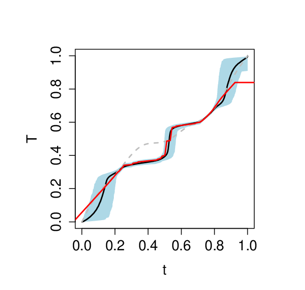
We start by illustrating our method on this setup on a single run-experiment; a Monte Carlo study was also conducted in this setting along the same lines as in Subsection 3.1 and it will also be reported below. A realisation of the original point process can be found in Figure 1. After estimating $F_{1},\dots,F_{n}$ using random Bernstein polynomials we obtain using (10) the posterior mean Fréchet mean depicted in Figure 4. The posterior mean is quite similar to the kernel-based estimator of Panaretos & Zemel 2016, and both are similar to the true Fréchet mean. Figure 4 also includes posterior inference for the warp functions. To examine the inference for warp functions in a greater level of detail Figure 5 presents the posterior mean Bernstein polynomial warp function along with credible bands for $i=5$. As it can be observed from the latter figure, our estimator follows closely that of Panaretos & Zemel 2016, and is reasonably in line with the original warp function; similar evidence holds for the remainder values of $i$ (see Figure 10). As expected, both estimators have however more difficulty in recovering the true value in the center of the unit interval but this is due to an extrapolation issue as there tends to be much less data on that region. Figure 5 also showcases that our method is more appropriate for bounded domains than the kernel as it takes full advantage of knowledge on the interval where the point processes lie.

Whilst the theoretical claims in Subsection 3.2 extend those of Panaretos & Zemel 2016—in the sense that under extra conditions they support the use of the methods even under a small $n$ large $m$ setting—numerical experiments in the supplementary materials suggest that the pointwise performance of our methods is tantamount to that of Panaretos & Zemel 2016. Figure 5 presents additionally credible intervals for randomly selected registered points for each registered point process. Observe that wider intervals are associated to points falling on the interval separating the two ‘clusters’ of points.

BG was partially supported by the graduate scholarship 21140901 from the Chilean NSF (CONICYT), YZ was supported by Swiss National Science Foundation Early Postdoc.Mobility Fellowship # 178220, and MdC was partially supported by FCT (Fundação para a Ciência e a Tecnologia, Portugal) through the projects PTDC/MAT-STA/28649/2017 and UID/MAT/00006/2019.

We begin by stating a number of auxiliary lemmata that will be useful to deriving our main results. Lemma 1 is often known as Pólya’s theorem (Lehmann & Romano 2006, Theorem 11.2.9). Lemma 2 states that inversion is continuous in supremum norm (Lehmann & Romano 2006, Lemma 11.2.1). Lemma 3 discusses sufficient conditions for (local) uniform convergence of the Bernstein polynomial density; see Ghosal & van der Vaart 2017 for a related result under further smoothness assumptions on $\mathbbm{f}$. As the proof of Lemma 3 shows, the uniform converges holds on any set bounded away from the discontinuity points of $\mathbbm{f}$. Proofs of Lemmata 1–3 are available from the supplementary materials.

Proof of Theorem 1.

1. (a)

   The proof follows from Theorem 3 in Petrone 1999b, combined with the fact that by assumption $F_{1},\ldots,F_{n}\iid\pi$. Indeed,

   $$\pi^{(n)}\{\mathscr{F}:\;\|F_{j}-\mathbb{F}_{j}\|_{\infty}<\varepsilon,\;j=1,\ldots,n\}=\prod_{j=1}^{n}\pi\{F_{j}:\|F_{j}-\mathbb{F}_{j}\|_{\infty}<\varepsilon\}>0.$$

2. (b)

   From (a) and Lemma 2 it follows that

   $$\pi^{(n)}\{\mathscr{F}:\|F_{i}^{-1}-\mathbb{F}^{-1}\|_{\infty}<\eta,i=1,\dots,n\}>0,\quad\eta>0.$$

   (6.14)

   Also, note that

   $$\|F^{-1}-\mathbb{F}^{-1}\|_{\infty}=\bigg\|\frac{1}{n}\sum_{i=1}^{n}F_{i}^{-1}-\mathbb{F}^{-1}\bigg\|_{\infty}\leq\frac{1}{n}\sum_{i=1}^{n}\|F_{i}^{-1}-\mathbb{F}^{-1}\|_{\infty}.$$

   (6.15)

   From (6.15) and Lemma 2, it follows that to have $\|F-\mathbb{F}\|_{\infty}<\varepsilon$ it would suffice having $\|F_{i}^{-1}-\mathbb{F}^{-1}\|_{\infty}<\delta$ for all $i$, thus implying that

   $$\pi^{(n)}\{\mathscr{F}:\|F-\mathbb{F}\|_{\infty}<\varepsilon\}\geq\pi^{(n)}\{\mathscr{F}:\|F_{i}^{-1}-\mathbb{F}^{-1}\|_{\infty}<\delta\}>0.$$

3. (c)

   Lemma 2 and the assumption $\mathbb{F}_{i}$ is (uniformly) continuous on $[0,1]$ imply that $\mathbb{F}_{i}^{-1}$ is also uniformly continuous, for $i=1,\dots,n$. Given $\eta>0$, let $\delta>0$ such that $|t-s|\leq\delta\Rightarrow|\mathbb{F}_{i}^{-1}(t)-\mathbb{F}_{i}^{-1}(s)|\leq\eta$, for $i=1,\dots,n$. From (a) and (b) it respectively follows that

   $$\pi^{(n)}\{\mathscr{F}:\|F_{i}^{-1}-\mathbb{F}^{-1}_{i}\|_{\infty}\leq\eta,\,i=1,\dots,n\}>0,\quad\pi^{(n)}\{\mathscr{F}:\|F-\mathbb{F}\|_{\infty}\leq\delta\}>0.$$

   Thus, $\pi^{(n)}\{\mathscr{F}:|F(x)-\mathbb{F}(x)|\leq\delta,\,x\in[0,1]\}>0$, and this implies that the event

   $$\begin{cases}F_{i}^{-1}(F(x))\leq F^{-1}_{i}(\mathbb{F}(x)+\delta)\leq\mathbb{F}_{i}^{-1}(\mathbb{F}(x)+\delta)+\eta\leq\mathbb{T}_{i}(x)+2\eta,\\ F_{i}^{-1}(F(x))\geq F^{-1}_{i}(\mathbb{F}(x)-\delta)\geq\mathbb{F}_{i}^{-1}(\mathbb{F}(x)-\delta)-\eta\geq\mathbb{T}_{i}(x)-2\eta,\\ \end{cases}$$

   (6.16)

   occurs with positive probability, for $i=1,\dots,n$. This thus yields that

   $$\pi^{(n)}\{\mathscr{F}:\|T_{i}-\mathbb{T}_{i}\|_{\infty}\leq 2\eta\}>0,\quad i=1,\dots,n.$$

4. (d)

   The strategy of the proof is similar to that of Panaretos & Zemel 2016. We start by noting that $T_{i}^{-1}\circ\mathbb{T}_{i}\in\Gamma(\Pi_{i}/N_{i},P_{i}/N_{i})$ as a consequence of

   $$\Pi_{i}=T_{i\;\#}^{-1}\widetilde{\Pi}_{i}=(T_{i}^{-1}\circ\mathbb{T}_{i})_{\#}P_{i},\quad i=1,\dots,n.$$

   It thus follows that

   $$\begin{split}d^{2}(\Pi_{i}/N_{i},P_{i}/N_{i})\leq\int_{0}^{1}\{(T_{i}^{-1}\circ\mathbb{T}_{i})(x)-x\}^{2}\,\frac{\Pi_{i}({\mathrm{d}}x)}{N_{i}}\leq\|\{T_{i}^{-1}\circ\mathbb{T}_{i}-x\}^{2}\|_{\infty}.\end{split}$$

   To complete the proof just note that (c) implies that for all $i$

   $$\pi^{(n)}\{\mathscr{F}:\|T_{i}^{-1}\circ\mathbb{T}_{i}-x\|_{\infty}<\varepsilon\}=\pi^{(n)}\{\mathscr{F}:\|T_{i}^{-1}-\mathbb{T}_{i}\|_{\infty}<\varepsilon\}>0,$$

   from where the final result follows.

Proof of Theorem 2. The derivatives of the induced priors (6) and (7) will be required for the proofs, and are respectively

1. (a)

   Let $\mathbbm{f}_{i}$ be the density corresponding to $\mathbb{F}_{i}$ and $\mathbbm{f}$ that corresponding of $\mathbb{F}$. Then

   $$|f(x)-\mathbbm{f}(x)|=n\left|\left(\sum_{i=1}^{n}\frac{1}{f_{i}(T_{i}(x))}\right)^{-1}-\left(\sum_{i=1}^{n}\frac{1}{\mathbbm{f}_{i}(\mathbb{T}_{i}(x))}\right)^{-1}\right|.$$

   (6.17)

   We first assume that $\inf\mathbbm{f}_{i}\geq 2l>0$ for all $i$, and consequently $\inf\mathbbm{f}>2l$ as well. For $g:[0,1]\to\mathbb{R}$ and $1/2>a>0$ denote $\|g\|_{\infty,a}=\sup_{x\in[a,1-a]}|g(x)|$. We shall show that the event

   $$\Omega_{a,\rho}=\{f_{i}\geq l\ \&\ \|f_{i}-\mathbbm{f}_{i}\|_{\infty,a}<\rho,i=1,\dots,n\},$$

   has positive probability for all $a,\rho>0$. Let $k_{i}$ be large so that $\|b(x\mid k_{i},\mathbbm{f}_{i})-\mathbbm{f}_{i}\|_{\infty,a}<\rho/2$ (using Lemma 3), set $k=\max_{i}k_{i}$ and denote $b(x\mid k,\mathbbm{f}_{i})=\sum_{j=1}^{k}w_{i,j}\beta(x\mid j,k-j+1)$. The set of polynomials with slightly perturbed coefficients

   $$\mathcal{P}_{i,\delta}=\left\{p=\sum_{j=1}^{k}w^{\prime}_{i,j}\beta(x\mid j,k-j+1):(w_{i,1}^{\prime},\dots,w_{i,k}^{\prime})\in S_{k}\text{ with }|w^{\prime}_{i,j}-w_{i,j}|<\delta,\text{for all }j\right\}$$

   has positive probability under the Bernstein polynomial prior, for all $\delta>0$, as a consequence of Petrone & Wasserman 2002 because the set where $(w^{\prime}_{i,1},\dots,w^{\prime}_{i,k})$ lies is open in the unit simplex. Moreover, each $p\in\mathcal{P}_{i,\delta}$ satisfies

   $$\|p-b(x\mid k,\mathbbm{f}_{i})\|_{\infty}\leq\delta k\max_{1\leq j\leq k}\sup_{x}\beta(x\mid j,k-j+1)<\infty$$

   because $1\leq j\leq k$. Thus for small enough $\delta$, $\|p-b(x\mid k,\mathbbm{F}_{i})\|_{\infty,a}<\rho/2$. Since the $F_{i}$’s are independent, there is a positive probability that $f_{i}\in\mathcal{P}_{i,\delta}$ for all $i$, which implies that $\|f_{i}-\mathbbm{f}_{i}\|_{\infty,a}<\rho$ for all $i$. Moreover, as $\mathbbm{f}_{i}\geq 2l$, $w_{i,j}\geq 2l/k$ and if $\delta<l/k$ this yields $w^{\prime}_{i,j}\geq l/k$ and thus $b(x\mid k,\mathbb{F}_{i})\geq l$. Hence $\Omega_{a,\rho}$ has positive probability.

   Fix $\epsilon>0$; we wish to show that $\|F_{i}-\mathbb{F}_{i}\|_{\infty}\leq\epsilon$ holds on $\Omega_{a,\rho}$ for appropriate $a,\rho>0$. Let $1/2>a>0$ such that $\mathbb{F}_{i}(a)<\epsilon/3$ and $\mathbb{F}_{i}(1-a)>1-\epsilon/3$, and let $\rho<\epsilon/3$. When $\Omega_{a,\rho}$ holds, we have

   	$\displaystyle 1\geq F_{i}(1-a)=F_{i}(a)+\int_{a}^{1-a}f_{i}(x)dx$	$\displaystyle\geq F_{i}(a)+\int_{a}^{1-a}\mathbbm{f}_{i}(x)dx-\rho(1-2a)$
   		$\displaystyle=F_{i}(a)+\mathbb{F}_{i}(1-a)-\mathbb{F}_{i}(a)-\rho(1-2a).$

   Thus $-\epsilon\leq F_{i}(a)-\mathbb{F}_{i}(a)\leq 1-\mathbb{F}_{i}(1-a)+\rho(1-2a)<2\epsilon/3$. For $x\leq a$ we have

   $$-\epsilon\leq F_{i}(x)-\mathbb{F}_{i}(x)\leq F_{i}(a)-\mathbb{F}_{i}(x)\leq 1-\mathbb{F}_{i}(1-a)+\rho(1-2a)+\mathbb{F}_{i}(a)-\mathbb{F}_{i}(x)\leq\epsilon.$$

   Thus $|F_{i}-\mathbb{F}_{i}|\leq\epsilon$ on $[0,a]$ and by a similar argument the same holds on $[1-a,1]$. For $x\in[a,1-a]$ observe that

   $$|F_{i}(x)-\mathbb{F}_{i}(x)|\leq|F_{i}(a)-\mathbb{F}_{i}(a)|+\int_{a}^{x}|f_{i}(y)-\mathbbm{f}_{i}(y)|dy\leq|F_{i}(a)-\mathbb{F}_{i}(a)|+\rho<\epsilon.$$

   Conclude that $\|F_{i}-\mathbb{F}_{i}\|_{\infty}\leq\epsilon$. As in the proof of Theorem 1 we have as a conseqeuence that for sufficiently small $a$ and $\rho$, on $\Omega_{a,\rho}$ $\|F_{i}^{-1}\circ F-\mathbb{F}_{i}^{-1}\circ\mathbb{F}\|_{\infty}<\epsilon$. Fix $a,\rho_{2}\in(0,1/2)$. Let $c_{i}=\min(\mathbb{F}_{i}^{-1}(\mathbb{F}(a)),1-\mathbb{F}_{i}^{-1}(\mathbb{F}(1-a)))$ and $a_{1}=\min_{i}c_{i}/2$. Since $\mathbbm{f}_{i}$ is uniformly continuous on $[a_{1},1-a_{1}]$, there exists $\delta_{2}>0$ such that $|\mathbbm{f}_{i}(x)-\mathbbm{f}_{i}(y)|\leq\rho_{2}$ for all $x,y\in[a_{1},1-a_{1}]$ such that $|x-y|\leq\delta_{2}$; without loss of generality $\delta_{2}\leq a_{1}$. Choose small $a_{1}>a_{2},\rho>0$ such that on $\Omega_{a_{2},\rho}$, $\|F_{i}^{-1}\circ F-\mathbb{F}_{i}^{-1}\circ\mathbb{F}\|_{\infty}<\delta_{2}$. Then on $\Omega_{a_{2},\rho}$

   $$\|f_{i}\circ F_{i}^{-1}\circ F-\mathbbm{f}_{i}\circ F_{i}^{-1}\circ F\|_{\infty,a}\leq\|f_{i}-\mathbbm{f}_{i}\|_{\infty,a_{1}}\leq\rho$$

   and

   $$\|\mathbbm{f}_{i}\circ F_{i}^{-1}\circ F-\mathbbm{f}_{i}\circ\mathbb{F}_{i}^{-1}\circ\mathbb{F}\|_{\infty,a}\leq\sup_{x,y\in[a_{1},1-a_{1}],|x-y|\leq\delta_{2}}|\mathbbm{f}_{i}(x)-\mathbbm{f}_{i}(y)|\leq\rho_{2}.$$

   This means that for any $\rho,\rho_{2},a>0$ there is positive probability that for all $i=1,\dots,n$

   $$\|f_{i}\circ F_{i}^{-1}\circ F-\mathbbm{f}_{i}\circ\mathbb{F}_{i}^{-1}\circ\mathbb{F}\|_{\infty,a}\leq\rho+\rho_{2},$$

   and since $\Omega_{a_{2},\rho}$ implies also that $f_{i},\mathbbm{f}_{i}\geq l$, it follows that for all $a,\epsilon>0$ there is positive probability that $\|f-\mathbbm{f}\|_{\infty,a}<\epsilon$. Now write

   $${\mathrm{KL}}(F,\mathbbm{F})=\int_{x\in[a,1-a]}\mathbbm{f}\log\frac{\mathbbm{f}}{f}+\int_{x\notin[a,1-a]}\mathbbm{f}\log\frac{\mathbbm{f}}{f}={\mathrm{KL}}_{1}+{\mathrm{KL}}_{2}.$$

   The definition of $\Omega_{a,\rho}$ implies that on this event $f\geq l$. Hence

   $${\mathrm{KL}}_{2}=\int_{x\notin[a,1-a]}\mathbbm{f}\log\mathbbm{f}-\int_{x\notin[a,1-a]}\mathbbm{f}\log f\leq\int_{x\notin[a,1-a]}\mathbbm{f}\log\mathbbm{f}-[1-F(1-a)+F(a)]\log l,$$

   and this vanishes as $a\to 0$ because $\int\mathbbm{f}\log\mathbbm{f}<\infty$. Hence we can pick $a>0$ such that ${\mathrm{KL}}_{2}<\epsilon$. To bound ${\mathrm{KL}}_{1}$ notice that when $\epsilon<l\leq\inf\mathbbm{f}$, and $\|f-\mathbbm{f}\|_{\infty,a}\leq\epsilon$, $\|\log\frac{\mathbbm{f}}{f}\|_{\infty,a}\leq\log\frac{\inf\mathbbm{f}}{\inf\mathbbm{f}-\epsilon}\leq\log\frac{l}{l-\epsilon}$. Thus, for all $\epsilon>0$ we have with positive probability

   $${\mathrm{KL}}(F,\mathbbm{F})\leq\epsilon+\log\frac{l}{l-\epsilon}.$$

   As this vanishes when $\epsilon\to 0$, the proof is complete under the assumption that $\inf\mathbbm{f}_{i}>0$ for all $i$. This assumption can be relaxed as in Petrone & Wasserman 2002^†† beware that they denote ${\mathrm{KL}}(F,\mathbbm{F})$ by ${\mathrm{KL}}(\mathbbm{F},F)$: take any $\mathbbm{f}$ as in the statement of the theorem and define $\mathbbm{f}^{a}(x)=\max(\mathbbm{f}(x),a)/A$, where $A=\int_{0}^{1}\max(\mathbbm{f}(x),a)dx\in[1,1+a]$. Then $\mathbbm{f}\leq A\mathbbm{f}^{a}$ and consequently $\int_{0}^{1}\mathbbm{f}^{a}(x)\log\mathbbm{f}^{a}(x)dx<\infty$. Applying the theorem to $\mathbbm{f}_{1}=\dots=\mathbbm{f}_{n}=\mathbbm{f}^{a}$ we deduce the KL property for $\mathbbm{f}^{a}$. Now, as $\mathbbm{f}\leq A\mathbbm{f}^{a}$ we have (Ghosal et al. 1999, Lemma 5.1)

   $${\mathrm{KL}}\bigg(\int h,\int\mathbbm{f}\bigg)\leq(A+1)\log A+A\left[{\mathrm{KL}}\left(\int h,\int\mathbbm{f}^{a}\right)+\sqrt{{\mathrm{KL}}\left(\int h,\int\mathbbm{f}^{a}\right)}\right].$$

   As $a\searrow 0$, $A\searrow 1$. If we choose $a>0$ such that $A<2$ and $(A+1)\log A<\varepsilon/3$, and then $\delta>0$ such that $\delta+\sqrt{\delta}<\varepsilon/3$ then

   $$\left\{h:{\mathrm{KL}}\left(\int h,\int\mathbbm{f}\right)\leq\varepsilon\right\}\supseteq\left\{h:{\mathrm{KL}}\left(\int h,\int\mathbbm{f}^{a}\right)\leq\delta\right\},$$

   and the latter has positive prior probability. This completes the proof.

2. (b)

   Again begin with the assumption that $\inf\mathbbm{f}_{i}>0$ for all $i$. Let $T_{i}^{\prime}(x)=f(x)/f_{i}(T_{i}(x))$ and $\mathbb{T}_{i}^{\prime}(x)=\mathbbm{f}(x)/\mathbbm{f}_{i}(\mathbb{T}_{i}(x))$, and note that

   $$|T_{i}^{\prime}(x)-\mathbb{T}_{i}^{\prime}(x)|\leq\frac{|f(x)-\mathbbm{f}(x)|}{f_{i}(T_{i}(x))}+\mathbbm{f}(x)\left|\frac{1}{f_{i}(T_{i}(x))}-\frac{1}{\mathbbm{f}_{i}(\mathbb{T}_{i}(x))}\right|.$$

   For all $a,\epsilon>0$, since $\mathbbm{f}$ is bounded on $[a,1-a]$, the same idea as in part (a) shows that with positive probability $\|T_{i}^{\prime}-\mathbb{T}_{i}^{\prime}\|_{\infty,a}<\epsilon$. Write again

   $${\mathrm{KL}}(T_{i},\mathbbm{T}_{i})=\int_{x\in[a,1-a]}\mathbbm{T}_{i}^{\prime}\log\frac{\mathbbm{T}_{i}^{\prime}}{T_{i}^{\prime}}+\int_{x\notin[a,1-a]}\mathbbm{T}_{i}^{\prime}\log\frac{\mathbbm{T}_{i}^{\prime}}{T_{i}^{\prime}}={\mathrm{KL}}_{1}+{\mathrm{KL}}_{2}.$$

   These two terms can be made small as in part (a) because $\mathbbm{T}_{i}^{\prime}\leq n$.

   To relax the condition $\inf\mathbbm{f}_{i}>0$ we use a similar idea as for part (a) but the argument is more subtle. Fix $a>0$ and define

   $$A_{i}=\int_{0}^{1}\max(\mathbbm{T}_{i}^{\prime}(x),a)\,{\mathrm{d}}x,\qquad h_{i}^{a}(x)=\max(\mathbbm{T}_{i}^{\prime}(x),a)/A_{i},\qquad H_{i}^{a}(x)=\int_{0}^{x}h_{i}^{a}(t)\,{\mathrm{d}}t.$$

   For brevity we omit the dependence of $h_{i}$, $H_{i}$ and $A_{i}$ on $a$. Clearly $H_{i}$ is strictly increasing, differentiable almost surely with derivative bounded below by $a/A_{i}$, $H_{i}(0)=0$ and $H_{i}(1)=1$. Moreover $h_{i}$ is continuous and strictly positive on $(0,1)$ because so is $\mathbbm{T}_{i}^{\prime}$. We shall view $H_{i}$ as transport maps from a Fréchet mean to well-behaved measures; first we need to fix the issue that they do not necessarily average to the identity by adding another transport map that corrects the discrepancy.

   By assumption

   $$A_{i}\leq\int_{0}^{1}(\mathbbm{T}_{i}^{\prime}(x)+a)dx=\mathbbm{T}_{i}(1)-\mathbbm{T}_{i}(0)+a=1+a$$

   and similarly $A_{i}\geq 1$. Thus we can choose $a>0$ small such that $(1+a)/A_{i}\leq 1+1/(2n)$ for all $i=1,\dots,n$. Define the correction function

   $$H_{n+1}(x)=(n+1)x-\sum_{i=1}^{n}H_{i}(x).$$

   Then $H_{i}$, $i=1,\dots,n+1$ average to the identity. Since $\mathbbm{T}_{i}$, $i=1,\dots,n$ average to the identity, whenever they are differentiable (that it, Lebesgue almost everywhere since they are nondecreasing) we have $\sum_{i=1}^{n}\mathbbm{T}_{i}^{\prime}(x)=n$. Hence $H_{n+1}$ is differentiable almost surely with derivative

   $$n+1-\sum_{i=1}^{n}h_{i}(x)\geq n+1-\sum_{i=1}^{n}\frac{\mathbbm{T}_{i}^{\prime}(x)}{A_{i}}-\frac{na}{A_{i}}\geq n+1-n\frac{1+a}{A_{i}}\geq n+1-n(1+\frac{1}{2n})=\frac{1}{2}.$$

   Now consider the distribution functions $\mathbb{G}_{i}=H_{i}^{-1}$, $i=1,\dots,n+1$ and let $\mathbb{G}$ denote the identity. Then $\mathbb{G}_{i}$ have Fréchet mean $\mathbb{G}$ with densities bounded above by $\max(2,A_{i}/a)$ and below by $1/(n+1)$. Therefore, by the previous part of the proof $H_{i}^{a}=\mathbb{G}_{i}^{-1}\circ\mathbb{G}$ is in the KL support of the induced Bernstein polynomial prior. Since $\mathbbm{T}_{i}^{\prime}\leq A_{i}h_{i}^{a}$ almost surely we have (Ghosal et al. 1999, Lemma 5.1)

   	$\displaystyle{\mathrm{KL}}(S,\mathbbm{T}_{i})$	$\displaystyle\leq(A_{i}+1)\log A_{i}+A_{i}[{\mathrm{KL}}(S,H_{i}^{a})+\sqrt{{\mathrm{KL}}(S,H_{i}^{a})}]$
   		$\displaystyle\leq(a+2)\log(a+1)+(a+1)[{\mathrm{KL}}(S,H_{i}^{a})+\sqrt{{\mathrm{KL}}(S,H_{i}^{a})}].$

   As $(H_{i}^{a})^{\prime}$ is continuous and strictly positive on $(0,1)$, ${\mathrm{KL}}(S,{H_{i}}^{a})$ can be made as small as we wish with positive probability. The fact that $a>0$ is arbitrary completes the proof.

References

- Agueh & Carlier (2011) Agueh, M. & Carlier, G. (2011). Barycenters in the Wasserstein space. Soc. Ind. Appl. Math. 43, 904–924.
- Barrientos et al. (2017) Barrientos, A. F., Jara, A. & Quintana, F. A. (2017). Fully nonparametric regression for bounded data using dependent Bernstein polynomials. Journal of the American Statistical Association 112, 806–825.
- Boissard et al. (2015) Boissard, E., Le Gouic, T. & Loubes, J.-M. (2015). Distribution’s template estimate with Wasserstein metrics. Bernoulli 21, 740–759.
- Ferguson (1973) Ferguson, T. S. (1973). A Bayesian analysis of some nonparametric problems. Ann. Stat. 1, 209–230.
- Ghosal et al. (1999) Ghosal, S., Ghosh, J. K. & Ramamoorthi, R. (1999). Consistent semiparametric Bayesian inference about a location parameter. Journal of Statistical Planning and Inference 77, 181–193.
- Ghosal & van der Vaart (2017) Ghosal, S. & van der Vaart, A. W. (2017). Fundamentals of Nonparametric Bayesian Inference. Cambridge University Press, Cambridge.
- Karr (1991) Karr, A. F. (1991). Point Processes and Their Statistical Inference. Probability: Pure and Applied. New York: Dekker, 2nd ed.
- Koenker (2005) Koenker, R. (2005). Quantile Regression. Cambridge, MA: Cambridge University Press.
- Lehmann & Romano (2006) Lehmann, E. L. & Romano, J. P. (2006). Testing Statistical Hypotheses. New York: Springer.
- Marron et al. (2015) Marron, J. S., Ramsay, J. O., Sangalli, L. M. & Srivastava, A. (2015). Functional data analysis of amplitude and phase variation. Statistical Science 30, 468–484.
- Menzel & Fabian (1999) Menzel, A. & Fabian, P. (1999). Growing season extended in Europe. Nature 397, 659.
- Panaretos & Zemel (2016) Panaretos, V. M. & Zemel, Y. (2016). Amplitude and phase variation of point processes. Ann. Stat. 44, 771–812.
- Panaretos & Zemel (2019) Panaretos, V. M. & Zemel, Y. (2019). Statistical aspects of Wasserstein distances. Annu. Rev. Stat. Appl. 6, 405–431.
- Petrone (1999a) Petrone, S. (1999a). Bayesian density estimation using Bernstein polynomials. The Canadian Journal of Statistics 27, 105–126.
- Petrone (1999b) Petrone, S. (1999b). Random Bernstein polynomials. Scandinavian Journal of Statistics 26, 373–393.
- Petrone & Wasserman (2002) Petrone, S. & Wasserman, L. (2002). Consistency of Bernstein polynomial posteriors. Journal of the Royal Statistical Society, Ser. B 64, 79–100.
- Peyré & Cuturi (2019) Peyré, G. & Cuturi, M. (2019). Computational optimal transport: With applications to data science. Foundations and Trends® in Machine Learning 11, 355–607.
- Ramsay & Silverman (2002) Ramsay, J. O. & Silverman, B. W. (2002). Applied Functional Data Analysis: Methods and Case Studies, vol. 77. New York: Springer.
- Ramsay & Silverman (2005) Ramsay, J. O. & Silverman, B. W. (2005). Functional Data Analysis. New York: Springer, 2nd ed.
- Santambrogio (2015) Santambrogio, F. (2015). Optimal Transport for Applied Mathematicians. Basel: Birkäuser.
- Schwartz et al. (2006) Schwartz, M. D., Ahas, R. & Aasa, A. (2006). Onset of spring starting earlier across the Northern Hemisphere. Global change biology 12, 343–351.
- Tang & Müller (2008) Tang, R. & Müller, H.-G. (2008). Pairwise curve synchronization for functional data. Biometrika 95, 875–889.
- Wang et al. (2016) Wang, J.-L., Chiou, J.-M. & Müller, H.-G. (2016). Functional data analysis. Annu. Rev. Stat. Appl. 3, 257–295.
- Wu et al. (2013) Wu, S., Müller, H. & Zhang, Z. (2013). Functional data analysis for point processes with rare events. Statistica Sinica 23, 1–23.
- Wu & Srivastava (2014) Wu, W. & Srivastava, A. (2014). Analysis of spike train data: Alignment and comparisons using the extended Fisher–Rao metric. Electron. J. Stat. 8, 1776–1785.
- Zemel & Panaretos (2019) Zemel, Y. & Panaretos, V. M. (2019). Fréchet Means and Procrustes Analysis in Wasserstein Space. Bernoulli 25, 932–976.
- Zheng et al. (2009) Zheng, Y., Zhu, J. & Roy, A. (2009). Nonparametric Bayesian inference for the spectral density function of a random field. Biometrika 97, 238–245.