Deep autoregressive neural networks for high-dimensional inverse problems in groundwater contaminant source identification

A common stochastic representation of a hydrological system can be written as

where $\bm{m}$ is a $N_{m}\times 1$ vector of the uncertain input parameters, $\bm{d}$ is a $N_{d}\times 1$ vector of the measurements, $f(\cdot)$ denotes the nonlinear forward model with input $\bm{m}$, and $\bm{e}$ is a vector of the measurement errors.

In ILUES (Zhang et al. 2018), the observation data are iteratively assimilated for multiple times. Rather than updating the ensemble of parameter realizations globally, ILUES employs a local update scheme to better handle strongly nonlinear and high-dimensional problems. More specifically, for an ensemble of $N_{e}$ parameter samples $\mathbf{M}=[\bm{m}_{1},\ldots,\bm{m}_{N_{e}}]$, it first identifies a local ensemble for each sample $\bm{m}_{i}\in\mathbf{M}$ based on a combined measure of the normalized distance to the measurements $\bm{d}$ and sample $\bm{m}_{i}$:

where $J_{d}(\bm{m})=[f(\bm{m})-\bm{d}]^{\top}\mathbf{C}_{\text{D}}^{-1}[f(\bm{m})-\bm{d}]$ is the distance between the model responses $f(\bm{m})$ and measurements $\bm{d}$, and $J_{m}(\bm{m})=(\bm{m}-\bm{m}_{i})^{\top}\mathbf{C}_{\text{MM}}^{-1}(\bm{m}-\bm{m}_{i})$ is the distance between the sample $\bm{m}_{i}$ and sample $\bm{m}\in\mathbf{M}$. Here, $\mathbf{C}_{\text{D}}$ is the $N_{d}\times N_{d}$ covariance matrix of the measurement errors $\bm{e}$, $\mathbf{C}_{\text{MM}}$ is the $N_{m}\times N_{m}$ autocovariance matrix of the input parameters in $\mathbf{M}$, $J_{d}^{\text{max}}$ and $J_{m}^{\text{max}}$ are the maximum values of $J_{d}(\bm{d})$ and $J_{m}(\bm{m})$, respectively. In earlier implementations of ILUES in Zhang et al. 2018, the local ensemble of $\bm{m}_{i}$ is the $N_{l}=\alpha N_{e},\;(\alpha\in(0,1])$ samples with the $N_{l}$ smallest $J$ values, i.e. $\mathbf{M}_{i}^{l}=[\bm{m}_{i,1},\ldots,\bm{m}_{i,N_{l}}]$, where $\alpha$ is the ratio between the sample sizes in $\mathbf{M}_{i}^{l}$ and $\mathbf{M}$. In this study, the local ensemble is determined using a roulette wheel selection operator (Lipowski and Lipowska 2012) based on the $J$ values, in which the selection probability of the $i$-th individual is given as $P_{i}=\rho_{i}/\sum_{j=1}^{N_{e}}\rho_{j}$, $i=1,\ldots,N_{e}$, where $\rho_{j}=1/J(\bm{m}_{j})$. This selection strategy may enhance the exploration of the parameter space in comparison to simply selecting the samples with the smallest $J$ values.

When assimilating the observation data, ILUES uses an inflated covariance matrix of the measurement errors to mitigate the large influence data mismatch at early iterations. The inflated covariance matrix is given by $\tilde{\mathbf{C}}_{\rm D}=\beta\mathbf{C}_{\rm D}$ and the factor $\beta$ is commonly chosen to be equal to the number of iterations $N_{\text{iter}}$ (Emerick and Reynolds 2012; Emerick and Reynolds 2013; Zhang et al. 2018). Let $n$ denote the iteration index ($n=0,\ldots,N_{iter}$), we first update the local ensemble of each sample $\bm{m}_{i}^{n}$ ($i=1,\ldots,N_{e}$), i.e., $\mathbf{M}_{i}^{l,n}$, by using the usual ES update scheme (Emerick and Reynolds 2013; Zhang et al. 2018):

for $j=1,\ldots,N_{l}$. Here $\mathbf{C}_{\text{MD}}^{l,n}$ is the cross-covariance matrix between $\mathbf{M}_{i}^{l,n}$ and $\mathbf{D}_{i}^{l,n}=\big[f(\bm{m}_{i,1}^{n}),\ldots,f(\bm{m}_{i,N_{l}}^{n})\big]$, $\mathbf{C}_{\text{DD}}^{l,n}$ is the autocovariance matrix of $\mathbf{D}_{i}^{l,n}$, and $\bm{d}_{j}=\bm{d}+\tilde{\mathbf{C}}_{\rm D}^{1/2}\bm{r}_{N_{d}}$, $\bm{r}_{N_{d}}\sim\mathcal{N}(\bm{0},\mathbf{I}_{N_{d}})$, is the $j$-th realization of the measurements. The update of $\bm{m}_{i}^{n}$ is then randomly selected from its updated local ensemble $\mathbf{M}_{i}^{l,{n+1}}=[\bm{m}_{i,1}^{n+1},\ldots,\bm{m}_{i,N_{l}}^{n+1}]$, say, $\bm{m}_{i,j}^{n+1}$ $(j=1,\ldots,N_{l})$. To accelerate the convergence of the ILUES algorithm, we add an additional accept-reject step to accept the updated sample with an acceptance rate:

Repeat this process for each sample $\bm{m}^{n}\in\mathbf{M}^{n}$ and the updated global ensemble $\mathbf{M}^{n+1}=[\bm{m}_{1}^{n+1},\ldots,\bm{m}_{N_{e}}^{n+1}]$ is obtained. The ILUES algorithm is summarized in Algorithm 1.

For high-dimensional inverse problems, large ensemble size and iteration number are required for ILUES to obtain converged and reliable inversion results (Zhang et al. 2018), leading to a large computational burden in forward model executions. To improve the computational efficiency, an accurate but fast-to-evaluate surrogate model constructed using a deep autoregressive neural network is used in this work to substitute the forward model in the ILUES algorithm.

DNNs are networks with a multi-layer structure (Goodfellow et al. 2016). Generally, given an input $\mathbf{x}$, the output of the $l$-th layer of a $L_{\rm{N}}$-layer network is given by

where $l$ denotes the layer index, $\eta(\cdot)$ is a nonlinear activation function, $\mathbf{W}^{(l)}$ and $\bm{b}^{(l)}$ are the weight matrix and bias vector, respectively, and $\mathbf{z}^{0}=\mathbf{x}$. In this work, the bias term is not considered, thus $\bm{\zeta}_{l}(\mathbf{z}^{(l-1)})=\eta_{l}(\mathbf{W}^{(l)}\mathbf{z}^{(l-1)})$.

For DNNs, fully-connected networks may lead to an extremely large number of network parameters. The convolutional network architecture is commonly employed to greatly reduce the network parameters due to its sparse-connectivity and parameter-sharing properties. In addition, convolutional neural networks are particularly suited for image-like data processing as the spatially-local dependence of the data is explicitly considered. More specifically, the layers of a convolutional neural network are organized into feature maps (matrices). Consider a two-dimensional input $\mathbf{x}\in\mathbb{R}^{H\times W}$, a convolutional layer, $\bm{\zeta}$, is obtained by employing a series of $q=1,\ldots,N_{\rm f}$ filters $\bm{\omega}^{q}\in\mathbb{R}^{k^{\prime}_{1}\times k^{\prime}_{2}}$, where $k^{\prime}$ is referred to as kernel size, to evolve an input pixel $x_{u,v}$ to obtain the feature value $\zeta_{u,v}^{q}(x_{u,v})$ at location $(u,v)$ by

This results in a convolutional layer consisting of $N_{\rm{f}}$ feature maps. The relationship between the output feature size $H_{\rm{fy}}\>(W_{\rm{fy}})$ and input feature size $H_{\rm{fx}}\>(W_{\rm{fx}})$ is given by (Dumoulin and Visin 2016)

where $s$ is the stride and $p$ is the zero padding that determine the distance between two successive moves of the filter and the padding of the borders of the input image with zeros for size preservation, respectively. Here, $\left\lfloor\cdot\right\rfloor$ represents the floor function.

In the DNN method considered here, an autoregressive strategy is proposed to improve the network’s performance in predicting the time-dependent response of the forward model with a time-varying source term. We adopt the dense convolutional encoder-decoder network architecture proposed in our previous work (Mo et al. 2018; Zhu and Zabaras 2018). It transforms the surrogate modeling task to an image-to-image regression problem to leverage the good properties of convolutional networks in image processing. In the following subsections, we briefly introduce the image-to-image regression strategy, the network architecture, and the deep autoregressive neural network. For the sake of completeness, in section 3.3.1, we summarize some elements of the work in Zhu and Zabaras 2018 and Mo et al. 2018.

In this section, a synthetic two-dimensional contaminant transport model revised after that of Zhang et al. 2015 is used to illustrate the performance of the proposed method. As shown in Figure 5, the spatial domain has a size of $10\;[\text{L}]\times 20\;[\text{L}]$ with constant heads of $h=1\;[\text{L}]$ and $h=0\;[\text{L}]$ at the left and right boundaries, respectively; whereas the two lateral boundaries are assumed to be no-flow boundaries. The domain is discretized uniformly into $41\times 81$ cells. During the time interval between $0\;[\text{T}]$ and $10\;[\text{T}]$, the contaminant is released with a time-varying strength from an unknown location within a potential area denoted by a white rectangle in Figure 5. The source strength is taken as the mass-loading rate $[\text{MT}^{-1}]$, i.e., the mass released in unit time. The unknown source is characterized by seven parameters, including the location $\bm{S}_{l}=(S_{lx},S_{ly})$, time-varying strengths $\bm{S}_{s}=\{S_{sj}\}_{j=1}^{5}$ in five time segments $[t_{j-1}:t_{j}]$, where $t_{j}=2j\;[\text{T}],\;j=1,\ldots,5$.

In this case, we assume that the porosity, longitudinal and transverse dispersivities are known with constant values of $\theta=0.25$, $\alpha_{L}=1.0\;[\text{L}^{2}\text{T}^{-1}]$ and $\alpha_{T}=0.1\;[\text{L}^{2}\text{T}^{-1}]$, respectively. The hydraulic conductivity field is heterogeneous and assumed to be a log-Gaussian random field, i.e.,

with a $L_{2}$ norm exponential covariance function:

where $\bm{s}=(s_{x},s_{y})$ and $\bm{s}^{\prime}=(s^{\prime}_{x},s^{\prime}_{y})$ are two arbitrary spatial locations, $m(\bm{s})=2$ is the constant mean, $\sigma_{G}^{2}=0.5$ is the variance, and $\lambda_{x}$ and $\lambda_{y}$ are the correlation lengths along the $x-$ and $y-$axes, respectively. In this example, we consider heterogeneous conductivity fields with a length scale of $\lambda/L_{\rm d}=0.2$ in both directions, where $L_{\rm d}$ is the domain size. Although the employed network architecture can effectively handle high-dimensional input fields even without using any dimensionality reduction techniques (Mo et al. 2018; Zhu and Zabaras 2018), an inverse problem with a high-input dimensionality will need a large number of forward model runs to obtain converged inversion results. Thus, to enable the implementation of the inversion method ILUES to relatively quickly obtain a converged solution, the Karhunen-Loève expansion (KLE) (Zhang and Lu 2004) is employed to parameterize the log-conductivity field, as represented by

where $\lambda_{i}$ and $\phi_{i}(\bm{s})$ are eigenvalues and eigenvectors of the convariance function, respectively, and $\xi_{i}\sim\mathcal{N}(0,1)$ are the KLE coefficients. The number of KLE terms required to preserve a specific percentage of the total field variance is determined by the length scale. A random field with a small length scale will vary highly over the domain and therefore a large number of KLE terms is required to accurately represent this high-variability (i.e., high-heterogeneity) feature. For the highly-heterogeneous field considered, we keep the first $N_{\text{KL}}=679$ dominant KLE terms to preserve $95\%$ of the total field variance (i.e., $\sum_{i=1}^{N_{\text{KL}}}\lambda_{i}/\penalty\sum_{i=1}^{\infty}\lambda_{i}\approx 0.95)$. As a result, in our inverse problem there are $N_{m}=686$ uncertain parameters, including $2$ source location parameters $(S_{lx},S_{ly})$, $5$ source strength parameters $\left\{S_{sj}\right\}_{j=1}^{5}$, and $679$ KLE coefficients $\left\{\xi_{i}\right\}_{i=1}^{679}$.

Although the dimensionality of the conductivity field $\mathbf{K}$ has been reduced from $3321$ (i.e., the number of spatial grids) to $679$ (i.e., the number of preserved KLE coefficients), in the ILUES algorithm, the input fed to the network is still the image-like conductivity field reconstructed from KLE. Figure 4 shows the procedure for making predictions for an arbitrary realization of the uncertain parameters $\bm{m}=(\bm{\xi},\bm{S}_{l},\bm{S}_{s})$. We first generate the conductivity field $\mathbf{K}$ using KLE based on the given coefficients $\bm{\xi}$ and the input images $\mathbf{S}\in\mathbb{R}^{5\times H\times W}$ for the source term $(\bm{S}_{l},\bm{S}_{s})$ as introduced in section 3.3.2; then based on the generated $\mathbf{K}$ and $\mathbf{S}$ the predicted output fields $\hat{\mathbf{y}}$ are obtained using the trained deep neural network.

The prior distributions of the $686$ unknown parameters are shown in Table 1. The $7$ uncertain source parameters are assumed to be uniformly distributed within the given ranges listed in Table 1. The $679$ KLE coefficients have a standard normal distribution, i.e., $\xi_{i}\sim\mathcal{N}(0,1)$. The randomly selected reference values for the $7$ source parameters and reference log-conductivity field are shown in Table 1 and Figure 5, respectively. To infer the unknown parameters, the concentrations at $t=[2,4,6,8,10,12,14]$ [T] and hydraulic heads are collected at $21$ measurement locations denoted by the black circles in Figure 5. Thus $N_{d}=21\times 8=168$ observations are available. The synthetic observations are generated by adding $5\%$ independent Gaussian random noise to the data generated by the forward model using the reference parameter values.

The concentration field usually has a large gradient in the region near the source release location due to small dispersivity. This strong nonlinearity is difficult to model and often leads to large approximation errors (Liao and Zhang 2013). To improve the network’s approximation accuracy in this region, in the loss function an additional weight $w_{c}$ is assigned to the source pixel (grid) and its surrounding eight pixels in the five concentration images at time $t_{1}$ to $t_{5}$ when the contaminant is released. As shown in Figure 7, according to the source location $(S_{lx},S_{ly})$, the concentrations at the source pixel and its surrounding eight pixels in the concentration field are extracted. Let $\bm{c}_{s}$ denote the vector of the nine concentrations extracted from one concentration field, the weighted loss can then be written as

where $J(\bm{\theta})$ is the $L_{1}$ loss as defined in equation (16), $n^{\prime}_{t}=5$ is the number of time segments that the contaminant is released, and $\hat{\bm{c}}_{s}$ is the network’s prediction for $\bm{c}_{s}$. A discussion on the choice of the value of weight $w_{c}$ is given in section 5.1.

To assess the effectiveness of the autoregressive strategy in improving the network’s approximation accuracy for the time series outputs of the contaminant transport model with a time-varying source term, and of the weighted loss in improving the characterization of the large-gradient concentration feature around the source release location, three types of networks are trained and compared:

Net: Network without autoregression. No autoregression is used in this network. It is trained using the original training samples without reorganizing the data using equation (15). That is, one model execution results in one training sample. The $L_{1}$ loss function defined in equation (16) is used.

AR-Net: Autoregressive network. In this network, the time-varying process is represented using an autoregressive model as defined in equation (13) and the network is trained using the reorganized training data as defined in equation (15). That is, one model execution results in $n_{t}$ reorganized training samples. The $L_{1}$ loss function defined in equation (16) is used.

AR-Net-WL: Autoregressive network with the weighted loss. AR-Net-WL is similar to AR-Net except that it is trained using a weighted loss function as defined in equation (23).

To illustrate the convergence of the approximation error with respect to the training sample size, three training sample sets obtained from $N=400$, $1000$, and $1500$ model evaluations are generated. The concentration at $t=[2,4,6,8,10,12,14]$ [T] and the hydraulic heads are taken as the observations for the inverse problem. Thus we collect the output concentration fields at the $n_{t}=7$ time instances $\{\mathbf{c}_{j}\}_{j=1}^{n_{t}}$ and the output hydraulic field $\mathbf{h}$ to train the network. The input to network is the hydraulic conductivity field $\mathbf{K}$ and the images $\{\mathbf{S}_{j}\}_{j=1}^{n_{t}}$ for the time-varying source term (see section 3.3.2). To assess the quality of the trained networks, $N_{\rm{test}}=500$ model runs are performed to generate the test samples. The quality is evaluated using the coefficient of determination ($R^{2}$) and the root mean squared error (RMSE) which are defined as

and

respectively. Here $\mathbf{y}^{i},\>\hat{\mathbf{y}}^{i}\in\mathbb{R}^{(n_{t}+1)\times H\times W}$ are the forward model and network predictions, respectively, for the hydraulic head field and $n_{t}$ concentration fields, and $\bar{\mathbf{y}}=1/N\sum_{i=1}^{N}\mathbf{y}^{i}$. A lower RMSE value and a $R^{2}$ score value approaching $1.0$ suggest better surrogate quality.

The differences between the autoregressive networks (i.e., AR-Net and AR-Net-WL) and the network without using the autoregressive strategy (i.e., Net) are summarized in Table 2. They include the number of input and output channels, and the batch size $M$. In Net, there are six input channels $\mathbf{x}\in\mathbb{R}^{6\times 41\times 81}$ and eight output channels $\mathbf{y}\in\mathbb{R}^{8\times 41\times 81}$, i.e., $\mathbf{x}=\big(\mathbf{K},\{\mathbf{S}_{j}\}_{j=1}^{5}\big)$ and $\mathbf{y}=\big(\mathbf{h},\{\mathbf{c}_{i}\}_{i=1}^{7}\big)$, where $\mathbf{h}$ is the hydraulic head field, and $\mathbf{c}_{i}$ is the concentration field at the $j$-th time step. In AR-Net and AR-Net-WL in which the training data are reorganized using equation (15), there are three input channels $\tilde{\mathbf{x}}\in\mathbb{R}^{3\times 41\times 81}$ and two output channels $\mathbf{y}\in\mathbb{R}^{2\times 41\times 81}$, i.e., $\tilde{\mathbf{x}}=(\mathbf{K},\mathbf{S}_{i},\mathbf{c}_{i-1})$ and $\mathbf{y}=(\mathbf{h},\mathbf{c}_{i})$, $i=1,\ldots,7$, where $\mathbf{c}_{0}=\mathbf{0}$ is the initial concentration. For the last two time intervals when no contaminant is released, the input image for the source term is zero at all pixels, i.e., $\mathbf{S}_{6}$, $\mathbf{S}_{7}=\mathbf{0}$. In Net, one training sample contains $7$ concentration fields at seven time steps, while in AR-Net and AR-Net-WL, one training sample contains only $1$ concentration field after reorganizing the training data. Thus, the batch size used in Net is $M=30$ and in AR-Net and AR-Net-WL is $M=200$.

The design of the network configuration follows Zhu and Zabaras 2018 and Mo et al. 2018 and the employed network architecture is shown in Table 3. The network is fully-convolutional consisting of $27$ layers. It contains three dense blocks with $L=5,\>10$ and $5$ internal layers, and a constant growth rate $R=40$. Three transition layers (one encoding layer and two decoding layers) are placed after each dense block. The number of initial feature maps after the first convolutional layer (the Conv in Figure 2) is $48$. The parameter values of the (transposed) convolution kernels (i.e., kernel size $k^{\prime}$, stride $s$, and zero-padding $p$) used in the dense blocks and transition layers are also listed in Table 3, where their values are denoted by the number in the right, e.g., for $k^{\prime}7s2p3$: $k^{\prime}=7$, $s=2$, and $p=3$. Since the value of concentration is always non-negative, the softplus function which is written as

is employed as the activation function of the output layer for the concentration to ensure non-negative predicted values, where $\beta=5$ is a shape parameter. In addition, the sigmoid function is used as the activation function of the output layer for the hydraulic head as its value varies between $0$ and $1$ in the case study. The initial learning rate $\varepsilon=0.005$ and weight decay $\omega_{d}=5\times 10^{-5}$. We also use a learning rate scheduler which drops ten times on plateau during the training process. The network is trained for $200$ epochs.

To determine a good value of the weight $w_{c}$ in the weighted loss (equation (23)) used in AR-Net-WL, six AR-Net-WL networks were trained using $400$ model evaluations with different weight values varying from $1.0$ to $50.0$ to test the effect of $w_{c}$ on the network’s performance. Figure 8 shows the RMSEs and $R^{2}$ scores of the six AR-Net-WLs evaluated on the test dataset. It is observed that the AR-Net-WLs with small $w_{c}$ values ($1.0$, $3.0$, $5.0$, and $10.0$) perform better than those with large $w_{c}$ values ($30.0$ and $50.0$). A large $w_{c}$ value promotes the training process to heavily focus on local refinement of the approximation for the large-gradient concentration region near the source release location, leading to a deterioration in the global approximation accuracy. Among the six trained AR-Net-WL networks, the one with $w_{c}=5.0$ performs well achieving a low RMSE value and a high $R^{2}$ score. Therefore, $w_{c}=5.0$ is selected for the remaining of our numerical studies.

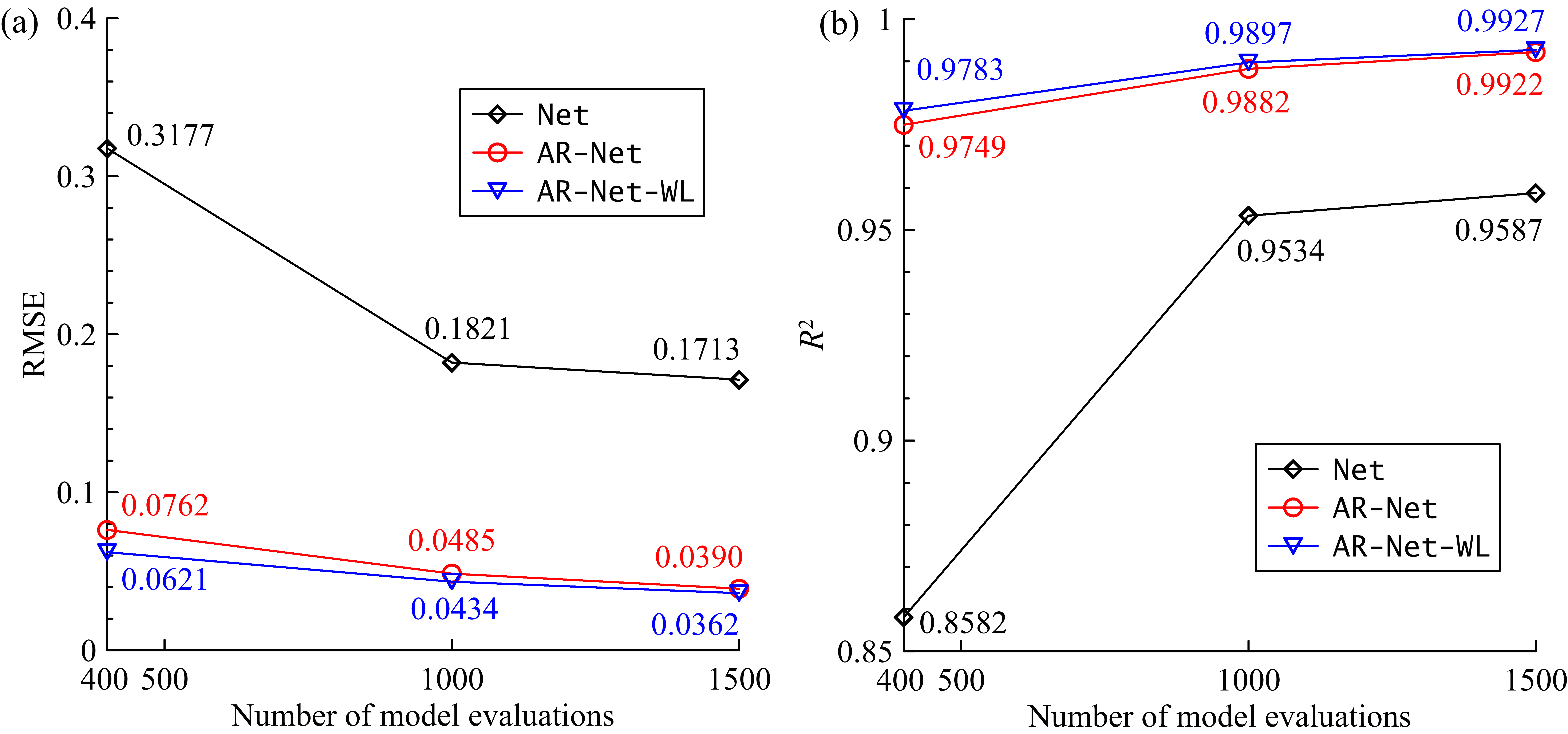
Next, we compare the performance of the Net, AR-Net, and AR-Net-WL networks trained using three different sample sizes ($N=400,1000,1500$). The networks are trained on a NVIDIA GeForce GTX $1080$ Ti X GPU. The training time of Net is about $6-18$ minutes for training $200$ epochs when the training sample size varies from $400$ to $1500$, and that of AR-Net and AR-Net-WL is about $32-110$ minutes. The increase in training time of AR-Net and AR-Net-WL is due to the number of training samples being increased to $n_{t}$ times the number of forward model runs after reorganizing the data. The networks’ RMSEs and $R^{2}$ scores evaluated on the test dataset are shown in Figure 9. For the solute transport system with a time-varying source release strength, the figure clearly demonstrates that the autoregressive networks AR-Net and AR-Net-WL achieve much lower RMSEs and much higher $R^{2}$ values than the Net network. For example, with $N=400$ forward model evaluations for network training, Net only achieves a RMSE value of $0.3177$ and $R^{2}$ value of $0.8581$, much lower than that of AR-Net and AR-Net-WL which achieve RMSE values of $0.0762$ and $0.0621$, and $R^{2}$ values of $0.9749$ and $0.9783$, respectively. With more training data available, the difference between the RMSEs and $R^{2}$ scores of the Net and AR-Net/AR-Net-WL decreases. With $1500$ forward evaluations for surrogate construction, AR-Net and AR-Net-WL can provide rather accurate approximations with $R^{2}$ scores of $0.9922$ and $0.9927$, respectively, for a problem with high-dimensional input and output fields. The results indicate that the autoregressive strategy employed in the AR-Net and AR-Net-WL networks substantially improves the network’s performance in approximating the solute transport system with a time-varying source term especially when the available training data are limited.

The performance of the networks is further compared in Figures 10, 11, and 12, which respectively show the predictions of Net, AR-Net, and AR-Net-WL using $N=400$ training samples for the concentration fields at $t=2,4,\ldots,14$ [T] and the hydraulic head field of a random test sample. For comparison, we also show the forward model predictions in each plot. Figure 10 shows that the predictions of Net have relatively large approximation errors for both the concentration and hydraulic head fields. For the concentration fields at the five time steps at $t=2,4,\ldots,10$ [T] when the contaminant is released, the approximation errors in the large-gradient region near the source release location are large relative to other regions. Figure 11 shows that AR-Net significantly reduces the approximation errors compared to those of Net. However, the approximation errors in the five concentration fields at $t=2,4,\ldots,10$ [T] near the source release location are still relatively large. In AR-Net-WL, we assign an additional weight of $w_{c}=5.0$ in the loss to the nine pixels around the source release location in the five concentration fields (equation (23)). Figure 12 indicates that the weighted loss in AR-Net-WL brings in an additional improvement in the characterization of this sharp-concentration feature without deteriorating the overall approximation accuracy. This improvement can also be demonstrated by Figure 9 which shows that AR-Net-WL achieves slightly lower RMSEs and higher $R^{2}$ scores than AR-Net when trained using the same three training datasets.

As can be seen from Figures 10-12, the maximum value of the absolute approximation errors, $|e_{c}|_{\max}=\max\big(|\mathbf{y}-\hat{\mathbf{y}}|\big)$, in each field of the $2500$ concentration fields at $t=2,4,\ldots,10$ [T] (i.e., the concentration fields at the $n^{\prime}_{t}=5$ time steps in the $N_{\rm test}=500$ test samples) usually occurs in the sharp-concentration region near the source release location. The improvement of AR-Net-WL compared to AR-Net in characterizing this sharp-concentration feature is further illustrated in Figure 13. It depicts a point-wise comparison of the $2500$ predictive values of $|e_{c}|_{\max}$ of the two networks trained with $N=400,1000$, and $1500$ in the $2500$ test concentration fields. An $(1:1)$ line is added in each plot to facilitate the comparison. A data point below (above) the $(1:1)$ line indicates that AR-Net has a larger (smaller) $|e_{c}|_{\max}$ value in a test concentration field than AR-Net-WL. It is observed that more data points are below the $(1:1)$ line in all three cases with $N=400,1000$, and $1500$, indicating AR-Net-WL’s overall better performance in approximating the sharp-concentration feature near the source release location. This can also be demonstrated in Table 4 which summarizes the mean and standard deviation of the $2500$ values of $|e_{c}|_{\max}$ obtained by the two networks. The table shows that the AR-Net-WL achieves lower means and standard deviations of $|e_{c}|_{\max}$ than AR-Net in all three cases with $N=400,1000$, and $1500$.