Fast post-hoc method for updating moments of large datasets
Abstract
Moments of large datasets utilise the mean of the dataset; consequently, updating the dataset traditionally requires one to update the mean, which then requires one to recalculate the moment. This means that metrics such as the standard deviation, correlation, and other statistics have to be ‘refreshed’ for dataset updates, requiring large data storage and taking long times to process. Here, a method is shown for updating moments that only requires the previous moments (which are computationally cheaper to store), and the new data to be appended. This leads to a dramatic decrease in data storage requirements, and significant computational speed-up for large datasets or low-order moments (n 10).
1 Introduction
This year, the Oak Ridge National Laboratory machine SUMMIT[1] exceeded 1.0 exaops ( operations per second) computational speed, bringing computing into the exascale era. In this era, scientific simulations will produce larger datasets than before, requiring large amounts of memory and data storage. In the plasma physics community, there has been much recent chatter about the strength of exascale computing and the associated data complications [2, 3]. Furthermore, the recent increase in popularity of machine learning and deep learning across a variety of different scientific sectors [4, 5, 6] has lead to a growing requirement to produce reduced metrics from datasets in an increasingly efficient fashion.
Computing moments with an updated dataset proves problematic for two reasons: the computational time taken to compute moments can scale with the size of the total data, and one has to retain a large amount of data in storage to compute new moments.
Here, we give an algorithm for computing moments of datasets which is instead computed in time proportional to the size of the data to be appended, and requires only a finite and typically small number of moments to be placed in data storage.
1.1 Definitions
We start by stating that we have a dataset containing data objects . Let us define the moment as the following:
| (1) |
where , and is the normalising function, defined here as the sum over of the weight function :
| (2) |
Accordingly, is equal to unity. is the weighted mean of the dataset , such that is identically zero:
| (3) |

1.2 Difficulties with calculating moments
Firstly, if one computes the original moment (1), this is completed in time. This is problematic, because if the dataset is updated times, then time is required on each update:
| (4) |
where is the total time taken. The time taken scales linearly with the number of updates, but also with the full dataset size. With data warehouses, this can lead to significant latency issues; in the limit that the increase in dataset size tends to zero, is still finite and non-zero.
This means that each update requires a full ‘refresh’ which discourages small updates, but also each update requires more computational time than any update before it.
Secondly, if one has a dataset which has moments calculated beforehand, the original information is lost; the mapping is many-to-one, and therefore the mapping is not invertible. This means that one requires an amount of available data storage given by:
| (5) |
where is the size of the data and is the size of the data . increases with each update, and means that we are required to use larger and large amounts of data to calculate these moments.
However, in principle, the moments themselves take up a much smaller amount of data storage :
| (6) |
where is the size of the data required to store each moment. For comparison, if , and are datatypes of the same size, then .
1.3 Dataset operations
We begin by defining operations on datasets. To do so, we will take the concept of datasets as a ‘vector’ and generalise the concept of vector space over a field (the field being the data objects, and the vector being the dataset); this will allow us to perform algebra using entire data structures, with a great deal of freedom in the available operations between data.
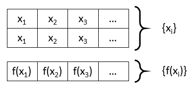
First, we define a dataset as a set of data objects . The dataset is categorized by the type of data objects that form the set, and the size of the dataset. The size of the dataset (cardinality) is referred to as .
It becomes useful to consider the data objects themselves as belonging to a field under addition and multiplication, which we will call the ‘datatype field’. That is to say, for data objects and belonging to a set corresponding to a given ‘datatype’:
| (7) |

The addition and multiplication operators ( and ) can be defined differently for different datatypes. For example, if we desire that the datatype is a set of cyclic numbers no bigger than 10, one might find:
whereas if the datatype were a set of a complex numbers:
Next, we define the data addition operator between two datasets and by the following:
| (8) |
Formally, the set of datasets and the data addition operator ‘’ form an Abelian group with identity element . There is no formal requirement for each member of to have the same datatype.
The data multiplication operator between two datasets is defined by the following:
| (9) |
The set of datasets and the data multiplication operator ‘’ form an Abelian group with identity element . As both groups are Abelian, one can now define a mathematical field formed by , data addition, and data multiplication. Exponentiation is simply an extension of multiplication:
| (10) |
It becomes useful to define a vector space over the field which the data objects belong to, using the field as elements of the vector space. Accordingly, for addition and multiplication:
For example, if is a set of 10 floating point numbers (floats), then the corresponding data structure is all possible sets of 10 floats. Operations between and another set of 10 floats are now defined, and each member of is a float.
Using a more complicated example, one can examine as a set of 10 lists, each containing 3 floats and 1 modulo number. In this case, is all possible combinations of 10 lists each with 3 floats and 1 modulo number, and each member of is a list of 3 floats and 1 modulo.
2 Primed moments
Suppose that we define the ‘updated’ dataset containing new values as such that:
| (11) |
is now said to have a cardinality of . The difference in cardinality is worth noting, and is herein referred to as :
| (12) |
We will also introduce the following shorthand:
| (13) |
2.1 Integer
For integer , the primed moment can be represented in the following form (see Appendix for proof):
| (14) |
where are binomial coefficients. can be determined using only a simple update:

| (15) |
which is computed in time. Similarly, can be computed in time:
| (16) |
The only points from that are required are the points not in ; viz. the only data required to update the moment is the new data. If all moments use the same amount of memory, then the data storage required is only:
| (17) |
This reduced data requirement leads to a computational speed up as well. The computational time taken per update is given by:
| (18) |
One quickly show that by comparing to (4) for speed up, one requires at worst:
| (19) |
This yields a threshold moment value:
| (20) |
For this value of or greater, (14) produces the primed moment slower than one could achieve using the original dataset; the speed-up is greatest for small updates to the dataset. However, in all cases, this method uses significantly less data storage.
2.2 Non-integer
For non-integer values of , one can use the fractional continuation of the binomial expansion:
| (21) |
Although it appears that the infinite sum is singular for , we have already assumed a priori that . As exists in a vector space, it has a well defined norm. We expect that the infinite sum is Abel convergent for , where denotes the Euclidean norm of the dataset on the vector space established in Section 1.3:
This condition is therefore related to the standard deviation of the original dataset. In short, we posit that for a set of data with a low standard deviation (), the infinite sum in (21) should converge. Therefore, one can truncate the sum so as to keep enough terms to yield the answer to a desired level of numerical accuracy:
| (22) |

where is the cutoff moment. Therefore, to numerical accuracy, one requires for data storage:
| (23) |
and the computational time taken per update is given by:
| (24) |
3 Weighted metrics
Suppose that we define the metric as:
| (25) |
where is an arbitrary function. Then, one can Taylor expand the function of the dataset around the mean value:
| (26) |
where are Taylor coefficients.
3.1 Updating metrics
If one updates the function , and the dataset then:
| (27) |
where denotes the new Taylor coefficients. This leads to a very powerful tool; provided that the moments of the original dataset are known it is possible for us to generate any arbitrary metric.
It is worth noting that if one rearranges for the change between and :
| (28) |
In principle, if one had , then this method is not particularly useful; we are essentially Taylor expanding at two different points (because the mean shifts), making our life much harder. This is not immediately intuitive; our expansion for employed here is always around the mean point of the dataset, rather than a free choice.
However, if is unknown and are known, then (27) is useful.
One can swap the order of summation on the first term. If one does so:


But as the binomial coefficients are monotonically increasing (at roughly ), the inside sum is not necessarily convergent. To guarantee Abel convergence, as should be monotonically increasing also, must satisfy:
| (29) |
This requirement means that we can only update via this method if the function has a convergent Taylor series. In such a case, one can use a cutoff for the first sum over in (27). Then:
| (30) |
The first term is iteratively calculated in time (such that one reaches numerical accuracy), while the second term is calculated in time.


4 Demonstration
Here, moments of datasets are compared using Python. Python forms a nice framework for adding data structures as one can freely redefine the addition and multiplication operators on objects of an arbitrary class. This makes the formalism from Section 1.3 easy to code, allowing us to simply add and multiple entire datasets as if they were just scalars.
4.1 Single precision floating point
For single precision floating points with boundaries at 0 and 1:
| (31) |
Two sets of floats, a 16 float set and a 256 float set were used to compute the original integer moments. Then, extra points were added to each set, and the new integer moments were calculated. For each speed test, a new, random set of floats were initialised using the numpy.random subpackage.
The scalar function is set to be a random map, such that each piece of data points to a random float. The random floats are reset for each speed test, just as the dataset is.
The speed-up was calculated by measuring the time taken to calculate the moment using the full dataset , and by using the update method given by (14). For each value of and moment, the timeit package was used to measure 100 runs of the algorithm.
As expected, the speed-up is less than 1 for high moments when the number of data points added () is large with respect to the size of the original dataset (). One finds that the maximum speed up (for the lowest order moment, ) is close to the theoretical maximum of a factor 16 speed up between the and the set, as shown in Figure 5.
4.2 List of single floats
We now examine a list of single floats. Using boundaries at 0 and 1 for each float, and setting the list length to 4:
| (32) |
The minimum update (in terms of ) now adds 4 floats to the dataset. In principle, this could be reformulated using the same analysis as in Section 4.1 but updating the dataset in groups of 4. As such, we expect that the speed-up will look very similar, but will be affected by the 4 fold global increase in datasize.
Again, we use numpy.random to generate a random set of floats, and is a random scalar map. As shown in Figure 6, the speed-up for 4 sets of 16 floats is fairly similar to that observed with a single set of 16 floats. However, when we increase to 4 sets of 256 floats, the speed up is much greater than the case where we examine a single set of 256 floats (see Figure 5). Again, one finds that the maximum speed up (for the lowest order moment, ) is close to the theoretical maximum of a factor 16.
5 Conclusion
In conclusion, this algorithm and method allows one to swiftly update moments and arbitrary metrics of datasets using less memory, and less data storage. The resultant code is lightweight, and can easily be implemented using class-oriented programming in a language of the readers’ choice (only Python results are shown here).
This algorithm is released as copyleft under the GNU GPL v3 license.
References
- [1] J. Hines. Stepping up to Summit. Computing in Science & Engineering, 20(2):78–82, 2018.
- [2] J-L Vay et al. Warp-X: a new exascale computing platform for plasma simulations. Bulletin of the American Physical Society, 2018.
- [3] D. Smith et al. Highlights from the community white paper “Enhancing US fusion science with data-centric technologies”. Bulletin of the American Physical Society, 2018.
- [4] B. K. Spears et al. Deep learning: A guide for practitioners in the physical sciences. Physics of Plasmas, 25(8):080901, 2018.
- [5] R. P. Eatough, N. Molkenthin, M. Kramer, A. Noutsos, M. J. Keith, B. W. Stappers, and A. G. Lyne. Selection of radio pulsar candidates using artificial neural networks. Monthly Notices of the Royal Astronomical Society, 407(4):2443–2450, 2010.
- [6] N. Coudray, P. S. Ocampo, T. Sakellaropoulos, N. Narula, M. Snuderl, D. Fenyö, A. L. Moreira, N. Razavian, and A. Tsirigos. Classification and mutation prediction from non–small cell lung cancer histopathology images using deep learning. Nature Medicine, 24(10):1559, 2018.
Appendix : Integer updates (proof)
To be demonstrated:
where is given by:
and is given by:
Proof.
From (1), one finds that after update:
| (A-33) |
where is given by:
| (A-34) |
First, if one examines :
such that the first term is the original value of the normalising function, and the second term represents the change in the value from adding new data.
If we split (A-34) into a sum over to , and to :
One finds that the following holds true:
where we have performed a binomial expansion of modified form of . By substituting the above into (A-33):
where we noted that .