The time evolution equation for advective heat transport as a constraint for optimal bounds in Rayleigh-Bénard convectionPreprint: APS/123-QED
Abstract
Upper bounds on the heat transport and other quantities of interest in Rayleigh-Bénard convection are derived in previous work from constraints resulting from the equations of time evolution for kinetic energy, the root mean square of temperature, and the temperature averaged over horizontal planes. Here, we investigate the effect of a new constraint derived from the time evolution equation for the advective heat transport. This additional constraint leads to improved bounds on the toroidal dissipation.
pacs
47.27.te, 44.25.+f, 92.60.FmI Introduction
Thermal convection is among the best studied problems of fluid mechanics. Its most basic idealization is Rayleigh-Bénard convection in which a fluid fills a plane layer infinitely extended in the horizontal directions, heated from below and cooled from above. The applied temperature difference, or the amplitude of the driving of the flow, is commonly expressed in terms of the Rayleigh number. Numerical simulations and experiments can investigate convection only up to a certain Rayleigh number. It is also possible to derive rigorous bounds on, for example, the heat transport across the convecting layer (Howard 1963; Busse 1969; Doering and Constantin 1996; Plasting and Ierley 2005; Seis 2015). The bounds derived in these references are valid at all Rayleigh numbers, but they tend to overestimate the actual heat transport. If power laws are fitted to both the bounds and numerically computed time averages, the fit to the bounds have a larger prefactor and usually a larger exponent. Furthermore, the bounds do not show any Prandtl number dependence.
These deficiencies arise because the derivation of the bounds does not exploit the full equations of evolution, but only a few integrals deduced from them: the energy budget, the relation between advective heat transport and dissipation, and the temperature equation integrated over horizontal planes. Seis Seis 2015 also makes use of the maximum principle for temperature. An improvement of the bounds necessarily requires to take advantage of additional constraints. This process is already well understood for systems of ordinary differential equations such as the Lorenz model Tobasco, Goluskin, and Doering 2018. In the context of convection, the implementation of further constraints is more cumbersome. Vitanov and Busse Vitanov and Busse 2000 split the energy budget into two equations, one for the poloidal and one for the toroidal energy. The resulting optimization problem preserves a dependence on the Prandtl number (and also on rotation if one is interested in rotating convection). But there is a price to pay in this approach. The optimization problem is not convex, and its Euler-Lagrange equations have to be solved numerically. Because of extensive coupling between different modes in a spectral decomposition of these equations, a numerical solution can only be obtained at low resolution, and hence at low Rayleigh numbers.
The approach pursued in this paper is to solve a semidefinite program (SDP). Previously obtained bounds on Rayleigh-Bénard convection can be reproduced by this method Tilgner 2017a. It has already been demonstrated how one can obtain increasingly sharp bounds on solutions of systems of ordinary differential equations by including more and more constraints Tobasco, Goluskin, and Doering 2018; Goluskin 2018. While the same systematic procedure is in principle possible for the Navier-Stokes equation Chernyshenko et al. 2014, it becomes unpractical for Rayleigh-Bénard convection even at modest Rayleigh numbers because all energy unstable modes need to be retained which leads to a large SDP. Fantuzzi et al. Fantuzzi, Pershin, and Wynn 2018 study bounds for Bénard-Marangoni convection and in this context discuss in depth limitations of the SDP approach and possible future lines of investigation. At present, the most straightforward approach remains to formulate an optimization problem in the form of an SDP with many decoupled linear matrix inequalities rather than a problem with a few, but large linear matrix inequalities. The goal of the present paper is to derive a Prandtl number dependent optimization problem for Rayleigh-Bénard convection which is convex and whose solution does not imply a significantly larger computational burden than optimization problems solved previously to find bounds on various observables of interest in Rayleigh-Bénard convection.
II The optimization problem
Let us consider the problem of Rayleigh-Bénard convection within the Boussinesq approximation for stress free boundaries. This choice of boundary conditions is not essential for obtaining the new constraint but it simplifies the calculation. A Cartesian coordinate system is chosen such that a plane layer is infinitely extended in the and directions and the boundaries of the layer are separated by the distance along the direction. Gravitational acceleration is acting along the negative direction. The layer is filled with fluid of density , kinematic viscosity , thermal diffusivity , and thermal expansion coefficient . Top and bottom boundaries are held at the fixed temperatures and , respectively. We will consider the equations of evolution immediately in nondimensional form, choosing for units of length, time, and temperature deviation from the quantities , and . With this choice, the equations within the Boussinesq approximation for the fields of velocity , temperature and pressure become:
| (1) | |||||
| (2) | |||||
| (3) |
In these equations, , so that represents the deviation from the conduction profile. The Prandtl number and the Rayleigh number are given by
| (4) |
and denotes the unit vector in direction. The boundary conditions on temperature require that at and 1 and the stress free conditions chosen here lead to at the boundaries.
It will be helpful to reduce the number of dependent variables by introducing poloidal and toroidal scalars and such that and is satisfied by construction. The component of the curl and the component of the curl of the curl of eq. (1) yield the equations of evolution for and ,
| (5) | |||||
| (6) |
with . For brevity, is not replaced by its expression in terms of and in these equations. The stress free boundary conditions translate into .
The currently known methods for obtaining upper bounds on fluid dynamic quantities cannot exploit the equations of evolution in full detail but extract averages from the original equations. Several types of averages will become important: the average over the entire volume, denoted by angular brackets without subscript, the average over an arbitrary plane , denoted by , and the average over time, which will be signaled by an overline.
Three useful relations between averages can now directly be obtained. The average of eq. (2) over planes leads to
| (7) |
Multiplication of eq. (2) with and a subsequent volume average yields
| (8) |
Finally, the dot product of with eq. (1), followed by a volume average, leads to
| (9) |
These three equations form the basis of the previous work on bounds on, for instance, the Nusselt number given by .
An additional relation will be derived below by computing from the time evolution equation of the advective heat transport . There are at least two reasons why such a relation looks promising. Bounds have been computed for double diffusive convection. In this problem, salinity drives convection together with temperature, and salinity obeys the same advection-diffusion equation as temperature except for a different diffusion constant. This problem looks superficially identical to ordinary convection and one may think that adding the equation for to the equations (7-9) provides us with enough information to derive bounds on double diffusive convection. In fact, it does not. It is necessary to include the equation for to derive bounds Balmforth et al. 2006. This demonstrates the usefulness of considering cross products of different physical quantities and motivates us to also look at . Another type of flows to which bounding methods were applied in the past are flows in periodic volumes driven by a body force . Doering and Foias 2002; Childress, Kerswell, and Gilbert 2001; Rollin, Dubief, and Doering 2011; Tilgner 2017b In these problems, it is essential to include the equation for obtained by forming the dot product of the momentum equation with . In Rayleigh-Bénard convection, the buoyancy force plays the role of the body force in the momentum equation. From this analogy, we have another reason to look at .
If we multiply the component of eq. (1) by , eq. (2) by , add the two equations and average the sum over the volume, we obtain the time evolution equation for the advective heat transport:
| (10) |
Thanks to the stress free boundary conditions and the boundary condition on temperature, one deduces from eq. (1) that at the boundaries. The divergence of eq. (1) yields . It is therefore possible to split the pressure into two terms and such that and
| (11) | |||||
| (12) |
with the boundary conditions that at and 1.
It will now be shown that the expression is quadratic in and positive. To this end, we first consider a layer with periodic boundary conditions and finite periodicity length in the lateral directions. At the end of the calculation, we will send the periodicity length to infinity in order to obtain the desired result for the infinitely extended layer. It helps to introduce two functions and defined by (so that ) and with the boundary conditions at and 1. These definitions imply that and are periodic in and and that at and 1. It is possible to compute , where the integration extends over the volume of a periodicity cell in the layer, by a sequence of integration by parts in which the boundary integrals all vanish:
| (13) | |||||
We can now divide this equation by the volume and take the limit to conclude that
| (14) |
where denotes the inverse Laplacian for homogeneous Dirichlet boundary conditions.
Before proceeding further, let us look at the form of the optimization problem which yields optimal bounds from eqs. (7-10). There are various ways to formulate such an optimization problem. The formulation presented here is most closely related to the method of auxiliary functions Chernyshenko et al. 2014; Chernyshenko 2017; Tobasco, Goluskin, and Doering 2018. To facilitate the exposition of the numerical implementation later, the formulation presented here is identical to ref. Tilgner 2017a. Suppose we want to bound some objective function which is defined in terms of the velocity and temperature fields. We chose test functions , , which depend only on and on which we project eq. (2):
| (15) |
We now construct the functional as
| (16) |
and replace all time derivatives by their expressions given in eqs. (8), (9), (15), and (10). The task now is to find a set of coefficients such that the inequality
| (17) |
holds for all fields , and which obey the free slip boundary conditions and at and 1. If such a set of ’s is found, the above inequality holds in particular for the fields taken from an actual time evolution. Taking the time average of relation (17) thus leads to . The time average of is zero because it is the linear combination of time derivatives. Replacing the time derivatives by their expressions in eqs. (8), (9), (15), and (10), the best upper bound for is given by the which solves the optimization problem
| (18) | ||||
with . The minimization occurs over all ’s and the inequality needs to hold for all and all eligible and .
This is nearly in a form which leads to an SDP after a suitable discretization. The problematic term is which involves a triple product in terms of , and . However, this term is readily reduced to a quadratic term by invoking the maximum principle which guarantees that in a statistically stationary state, the temperature takes on values in the interval bounded by the temperatures at the top and bottom planes of the layer, which means that , or equivalently, .
To make best use of the maximum principle, we want to compute in the form . This expression can be simplified with the same artifice as before: we first integrate over a volume with periodic boundary conditions in the horizontal before taking the limit . The second term of the above expression requires us to compute
| (19) |
in which only the horizontal average of appears which obeys
| (20) | |||||
We can thus solve with the boundary conditions that at and 1 to find since at and 1. Inserting this into eq. (19) yields
| (21) |
after another integration by parts.
The only triple product left in problem (18) is . This can be reduced to a quadratic term only at the price of an inequality:
| (22) |
The last expression is quadratic in and could be combined with (18) to obtain a convex optimization problem which can be represented as an SDP for numerical purposes. However, the solution of this problem would be very expensive. The success of the previous applications of semidefinite programming to Rayleigh-Bénard convection Tilgner 2017a relied on the fact that if the dependence in and is represented as Fourier series, the equations decouple in the wavenumber of the Fourier modes and only a small number of amplitudes of Fourier modes needs to be taken into account in a numerical computation. The term unfortunately destroys that decoupling.
The decoupling can be restored at the expense of a further inequality. It is shown in the appendix that
| (23) |
Inserting this into eq. (22), and (22) together with (21) into (18), leads to the following optimization problem for the optimal bound of the objective function , where the minimum is sought over all ’s:
| (24) | ||||
The last line implies . Since the right hand side of the first inequality constraint in (24) is positive, is smallest when is chosen as small as possible, which implies that at optimum. The velocity field is left as a variable in (24) so that it is easier to trace the various terms to the preceding development, but eventually, is replaced by and
.
Problem (24) contains eq. (10) as a constraint which keeps as a parameter in the optimization. The effect of is expected to be strongest for . It will be of interest to also study a reduced optimization problem which results from (24) by introducing , . The dissipation is known to be bounded uniformly in , Howard 1963; Busse 1969; Doering and Constantin 1996 so that in the limit , the right hand side of the inequality constraint disappears and we are left with a simpler problem:
| (25) | ||||
The virtue of this formulation is that it is independent of any sloppiness that may have eased the derivation of eq. (23). The optimization (25) would not be changed by a sharper inequality than (23).
The numerical solution of problems (24) and (25) proceeds in exactly the same way as in ref. Tilgner 2017a so that a brief summary will suffice here. The variables and are decomposed into Chebychev polynomials for the direction and into plane waves in and , as for example in
| (26) |
The test functions are chosen as delta functions centered at the collocation points defined by
| (27) | |||||
| (28) |
Inserting all this into the optimization problems transforms the inequality constraints into the condition that some symmetric matrix be positive semidefinite. This is the standard form of an SDP. The constraints decouple in . Only a small number of wavenumbers actually constrain the solution. This set of wavenumbers is determined automatically Tilgner 2017a. The matrix occurring in the SDP would be much larger if the constraints did not decouple in , hence the effort put into obtaining eq. (23). Some improvements of the basic method accelerate the computation but are not essential. These include a partial integration of eq. (15) and the exploitation of symmetry in . Tilgner 2017a The resulting SDP was solved with the package cvxopt.


III Results
The optimization problem (24) distinguishes itself from previous problems by the terms multiplied by and , which include all the terms containing . In order to test the power of the new constraint, it seems best to choose an objective function which varies dramatically as a function of . The dissipation of the non poloidal components fulfills this criterion, because the flow is purely poloidal at infinite , whereas it contains both poloidal and toroidal components at finite . The choice thus promises to be a gratifying objective function.
Call the optimal of problem (24) for . Fig. 1 shows as a function of for different . It is seen that is constant for low until it monotonically decreases as a function of and asymptotes towards a value different from zero at high . The optimization problem (24) thus is not powerful enough to show that the toroidal dissipation disappears at infinite . Let us denote with the value of at small and with the limiting value of as tends to infinity. and are functions of .
is equal to the upper bound one obtains without the constraint derived from , or with in (24). This bound is the same as the one computed in ref. Tilgner 2017a and obeys approximately at high . The new constraint introduced in this paper becomes active and reduces the upper bound for . From plots like fig. 1 one finds as a function of , which is shown in fig. 2. needs to be larger than to obtain improved bounds.

Just as can be computed from a simplified optimization problem, so can be computed from the reduced problem (25) which has the advantage that it does not depend on any more, and it is independent of how sharp the estimate in (23) is. is the lowest bound found for any at a given , so that is a measure of the maximum fractional improvement of the bound due to the additional constraint (10) at the given . This fraction is shown in fig. 3. As can be seen from this figure, the constraint (10) can improve the bound by more than a factor of 2 at small , but dishearteningly, the improvement vanishes for large . Bounding methods should be useful at high when ordinary time integrations become too expensive. But it is precisely in this limit that the newly added constraint does not improve the previously known bound.
The objective function most often considered in the context of optimum theory is , which is the Nusselt number minus one. With this choice, the fractional improvement of previous known bounds is found to be less than , and since this is less than the tolerances and errors in the numerical procedure, the improvement could be exactly zero. The potential improvement is at any rate so small that it was not considered worthwhile to determine it accurately, or to show that it vanishes.
IV Conclusion
Previous work has derived bounds on the Nusselt number or other flow quantities in convection from the time evolution equations for , , and . The present paper adds to the list. This additional constraint does not improve the bounds on the Nusselt number by an unambiguously detectable amount. The bounds on the toroidal dissipation on the other hand can be improved by more than , but there is no improvement at large . This fact is remarkable because it contradicts the behavior one may intuit from other results in the optimum theory of turbulence. In order to derive bounds for flows in 3D periodic boxes driven by a body force , it is necessary to take into account the time evolution equation for . For convection within the Boussinesq approximation, the momentum equation contains a driving term proportional to . The term analogous to of the 3D periodic box is therefore . For an immediate analogy with previous work, the forcing should be solenoidal, so that we should first consider , where is chosen such that . However, for a solenoidal velocity field with zero normal component at the boundaries, the expression reduces to . It is therefore surprising that there is not a more striking improvement of bounds for convective flows if the time evolution equation of is included in the optimization problem. At finite , the bounding problem relies on inequality (23) which can possibly be improved. In the limit of large , however, the results are independent of this inequality and no improvement of the results presented here can be achieved without adding yet another constraint.
*
Appendix A
The goal of this appendix is to prove eq. (23). To this end, we have to compute , where is an arbitrarily large volume in the plane layer, and is given by
| (29) |
with at and 1. The variable is used as an abbreviation for . We will proceed by finding the Green’s function such that so that where the integral extends over the horizontally infinitely extended layer. Once the Green’s function is known, we can estimate the desired integral from
| (30) | |||||
and taking the limit :
| (31) |
Because of the translational invariance, the last factor in eq. (31) simplifies to
| (32) |
The Green’s function for eq. (29) with Neumann boundary conditions describes for example the potential flow out of a point source in a plane layer. The maximization in expression (32) asks for the distance from the lower boundary of the layer at which one has to place the point source so that the absolute value of the component of the velocity integrated over the entire layer is maximum. One intuitively expects that the maximum is reached when the point source is located on one of the boundaries of the layer. It seems very likely that the Green’s function for exactly this problem is given somewhere in the existing literature, but I was not able to find a suitable reference. However, the Green’s function for eq. (29) with the Dirichlet boundary conditions at and 1 describes the electrostatic potential of a point charge between two parallel infinitely extended metallic plates kept at zero potential, and the Green’s function for this electrostatic problem can be found in the textbook by Jackson Jackson 1999. Adapting the result in this textbook from Dirichtlet to Neumann boundary conditions leads to
| (33) |
where the position is given in cylindrical coordinates and is a constant left unspecified by the Neumann boundary conditions and which is irrelevant because we are only interested in . is a modified Bessel function of the second kind in the usual notation.

We will abstain from formal proofs for two properties which we will deduce from numerical evaluation of eq. (33) and which match the intuition about one may have from its interpretation as a potential flow out of a point source. The first observation concerns the at which the maximum in (32) is realized. Fig. 4 shows as a function of computed numerically from the first 40 terms of eq. (33). As expected, this integral is maximal for (or by symmetry). The value of the maximum is numerically close to .
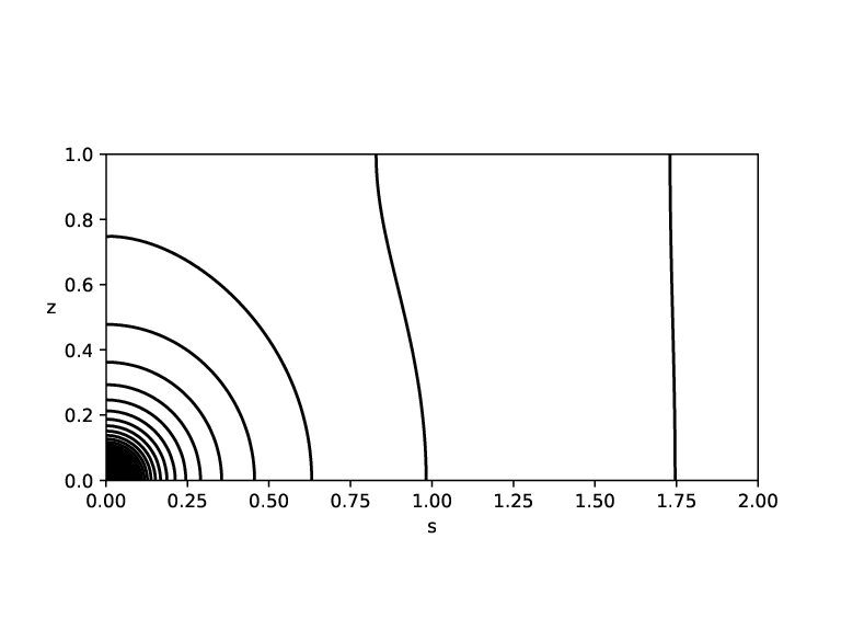
This second point can be made more precise with the help of a weaker observation. Let us introduce for brevity as the Green’s function corresponding to a point source located at the origin, . A contour plot of in cylindrical coordinates is shown in fig. 5. The second property to extract from numerical calculation and which is again expected from the interpretation of as potential flow, is that has the same sign everywhere. This second property is important because it implies that we can avail ourselves of the absolute values in expression (32). Using the formulas and , one finds
| (34) | |||||
so that eq. (31) leads to
| (35) |
For solenoidal fields , this can be brought into a form which is more pleasant for the SDP:
| (36) | |||||
which in the limit leads to eq. (23).
References
- Howard (1963) L. Howard, “Heat transport by turbulent convection,” J. Fluid Mech. 17, 405–432 (1963).
- Busse (1969) F. Busse, “On Howard’s upper bound for heat transport by turbulent convection,” J. Fluid Mech. 37, 457–477 (1969).
- Doering and Constantin (1996) C. Doering and P. Constantin, “Variational bounds on energy dissipation in incompressible flows:III. Convection,” Phys. Rev. E 53, 5957–5981 (1996).
- Plasting and Ierley (2005) C. Plasting and G. Ierley, “Infinite-Prandtl-number convection. Part 1. Conservative bounds,” J. Fluid Mech. 542, 343–363 (2005).
- Seis (2015) C. Seis, “Scaling bounds on dissipation in turbulent flows,” J. Fluid Mech. 777, 591–603 (2015).
- Tobasco, Goluskin, and Doering (2018) I. Tobasco, D. Goluskin, and C. Doering, “Optimal bounds and extremal trajectories for time averages in dynamical systems,” Phys. Lett. A 382, 382 – 386 (2018).
- Vitanov and Busse (2000) N. Vitanov and F. Busse, “Bounds on the convective heat transport in a rotating layer,” Phys. Rev. E 63, 016303 (2000).
- Tilgner (2017a) A. Tilgner, “Bounds on poloidal kinetic energy in plane layer convection,” Phys. Rev. Fluids 2, 123502 (2017a).
- Goluskin (2018) D. Goluskin, “Bounding averages rigorously using semidefinite programming: mean moments of the Lorenz system,” Journal of Nonlinear Science 28, 621–651 (2018).
- Chernyshenko et al. (2014) S. Chernyshenko, P. Goulart, D. Huang, and Papachristodoulou, “Polynomial sum of squares in fluid dynamics: a review with a look ahead,” Phil. Trans. Roy. Soc. A 372, 20130350 (2014).
- Fantuzzi, Pershin, and Wynn (2018) G. Fantuzzi, A. Pershin, and A. Wynn, “Bounds on heat transfer for Bénard-Marangoni convection at infinite Prandtl number,” J. Fluid Mech. 837, 562–596 (2018).
- Balmforth et al. (2006) N. Balmforth, S. Ghadge, A. Kettapun, and S. Mandre, “Bounds on double-diffusive convection,” J. Fluid Mech. 569, 29–50 (2006).
- Doering and Foias (2002) C. Doering and C. Foias, “Energy dissipation in body-forced turbulence,” J. Fluid Mech. 467, 289–306 (2002).
- Childress, Kerswell, and Gilbert (2001) S. Childress, R. Kerswell, and A. Gilbert, “Bounds on dissipation for Navier-Stokes flow with Kolmogorov forcing,” Physica D 158, 105–128 (2001).
- Rollin, Dubief, and Doering (2011) B. Rollin, Y. Dubief, and C. Doering, “Variations on Kolmogorov flow: turbulent energy dissipation and mean flow profiles,” J. Fluid Mech. 670, 204–213 (2011).
- Tilgner (2017b) A. Tilgner, “Scaling laws and bounds for the turbulent G.O. Roberts dynamo,” Phys. Rev. Fluids 2, 024606 (2017b).
- Chernyshenko (2017) S. Chernyshenko, “Relationship between the methods of bounding time averages,” arXiv:1704.02475 (2017).
- Jackson (1999) J. Jackson, Classical Electrodynamics, 3rd edition (Wiley, New York, 1999).