Computation of the spectrum of $\text{dc}^{2}$-balanced codes Thanks: Kees A. Schouhamer Immink is with Turing Machines Inc, Willemskade 15d, 3016 DK Rotterdam, The Netherlands. E-mail: immink@turing-machines.com. Thanks: Kui Cai is with Singapore University of Technology and Design (SUTD), 8 Somapah Rd, 487372, Singapore. E-mail: cai_kui@sutd.edu.sg.Thanks: This work is supported by Singapore Agency of Science and Technology (A*Star) PSF research grant and SUTD-ZJU grant ZJURP1500102

The number of $\text{dc}^{2}$-balanced codewords, $x$, $N_{\text{dc}^{2}}(x_{i_{0}}=x_{i_{1}}=1)$, that is required for computing the auto-correlation function using (13) and (14), can be computed using generating functions. For very large $n$, however, this rapidly becomes an impractically cumbersome exercise, and an efficient alternative method is considered a desideratum.

To that end, we exploit the central limit theorem by regarding the integer variables $x_{i}\in\{0,1\}$ as i.i.d. binary random variables whose numerical outcomes ‘0’ or ‘1’ are equally likely. We define the stochastic variables $c$ and $p$ by

$$c=x_{1}+x_{2}+\cdots+x_{n}$$

(15)

and

$$p=x_{1}+2x_{2}+\cdots+nx_{n},$$

(16)

where $x_{i_{0}}=x_{i_{1}}=1$, $i_{0},i_{1}\in\{1,\ldots,n\}$.

The central limit theorem [23], Chapter 8, states that for asymptotically large $n$ the distribution of the stochastic variables $c$ and $p$, which are obtained by summing a large number, $n$, of independent stochastic variables, approaches a two-dimensional Gaussian distribution.

Let $E[.]$ denote the expected value operator for all possible codewords in $S_{2}$. Let the parameters $\mu_{c}=E[c]$ and $\mu_{p}=E[p]$ denote the average of $c$ and $p$, and let $\sigma_{c}^{2}=E[(c-\mu_{c})^{2}]$ and $\sigma_{p}^{2}=E[(p-\mu_{p})^{2}]$ denote the variance of $c$ and $p$. The parameter $r$ denotes the linear correlation coefficient between the random variables $c$ and $p$. Then the bi-variate Gaussian distribution, denoted by $G(c,p)$, is given by

$$G(c,p)=\frac{1}{2\pi\phi_{1}}e^{-\phi(c,p)},$$

(17)

where

$$\phi^{2}_{1}=\sigma^{2}_{c}\sigma^{2}_{p}(1-r^{2}),$$

(18)

$$\phi(c,p)=\frac{1}{2(1-r^{2})}f(c,p),$$

(19)

and

$$f(c,p)=\left(\frac{c-\mu_{c}}{\sigma_{c}}\right)^{2}+\left(\frac{p-\mu_{p}}{\sigma_{p}}\right)^{2}-\frac{2r(c-\mu_{c})(p-\mu_{p})}{\sigma_{c}\sigma_{p}}.$$

We have

$$E[x_{i}]=E[x^{2}_{i}]=\frac{1}{2},\mbox{ and }E[x_{i}x_{j}]=\frac{1}{4},\,\,i\neq i_{0},i_{1},$$

(20)

$$E[x_{i}]=E[x^{2}_{i}]=1,\,i=i_{0},i_{1},\,E[x_{i}x_{j}]=\frac{1}{2},\,i,j=i_{0},i_{1},$$

and $E[x_{i_{0}}x_{i_{1}}]=1$. We may find after a routine computation using (20) that

$$\mu_{c}=E\left[\sum_{i=1}^{n}x_{i}\right]=\sum_{i=1}^{n}E[x_{i}]=\frac{n-2}{2}+2$$

and similarly

$$\mu_{p}=E\left[\sum_{i=1}^{n}ix_{i}\right]=\sum_{i=1}^{n}E\left[ix_{i}\right]=\frac{n(n+1)}{4}+\frac{i_{0}+i_{1}}{2}.$$

The variances $\sigma_{c}^{2}$, $\sigma_{p}^{2}$, and the correlation coefficient $r$ can be found without too much difficulty:

$$\sigma^{2}_{c}=E\left[\sum_{i=1}^{n}(x_{i}-\mu_{c})^{2}\right]=\frac{n-2}{4},$$

(21)

	$\displaystyle\sigma_{p}^{2}$	$\displaystyle=$	$\displaystyle E\left[\sum_{i=1}^{n}(ix_{i}-\mu_{p})^{2}\right]$		(22)
		$\displaystyle=$	$\displaystyle\frac{n(n+1)(2n+1)}{24}-\frac{i_{0}^{2}+i_{1}^{2}}{4},$

and

	$\displaystyle r^{2}$	$\displaystyle=$	$\displaystyle\frac{E[\sum_{i=1}^{n}(x_{i}-\mu_{c}).\sum_{i=1}^{n}(ix_{i}-\mu_{p})]}{\sigma^{2}_{c}\sigma_{p}^{2}}$		(23)
		$\displaystyle=$	$\displaystyle\frac{3}{2(n-2)}\frac{(n^{2}+n-2(i_{0}+i_{1}))^{2}}{2n^{3}+3n^{2}+n-6(i_{0}^{2}+i_{1}^{2})}.$

The total number of $n$-sequences with $x_{i_{0}}=x_{i_{1}}=1$, equals $2^{n-2}$, so that for asymptotically large $n$, the number of $n$-sequences versus $c$ and $p$, denoted by $N(c,p;x_{i_{0}}=x_{i_{1}}=1)$, can be approximated by

$$N(c,p;x_{i_{0}}=x_{i_{1}}=1)\sim 2^{n-2}G(c,p)=\frac{2^{n}}{8\pi\phi_{1}}e^{-\phi(c,p)}.$$

(24)

A $\text{dc}^{2}$-balanced codeword satisfies, by definition, the conditions, see (5), $c=n/2$ and $p=n(n+1)/4$. Then, $N_{\text{dc}^{2}}(x_{i_{0}}=x_{i_{1}}=1)$ is found after substituting $c=n/2$ and $p=n(n+1)/4$ into (24). We find

$$N_{\text{dc}^{2}}(x_{i_{0}}=x_{i_{1}}=1)\sim\frac{2^{n}}{8\pi\phi_{1}}e^{-\phi_{2}},$$

(25)

where, see (18) and (19),

	$\displaystyle\phi_{2}$	$\displaystyle=$	$\displaystyle\phi\left(c=\frac{n}{2},p=\frac{n(n+1)}{4}\right)$		(26)
		$\displaystyle=$	$\displaystyle\frac{1}{2(1-r^{2})}\left\{\left(\frac{1}{\sigma_{c}}\right)^{2}+\left(\frac{i_{0}+i_{1}}{2\sigma_{p}}\right)^{2}-\frac{r(i_{0}+i_{1})}{\sigma_{c}\sigma_{p}}\right\}$
		$\displaystyle=$	$\displaystyle\frac{4\sigma^{2}_{p}+\sigma^{2}_{c}(i_{0}+i_{1})^{2}-4r\sigma_{c}\sigma_{p}(i_{0}+i_{1})}{8\phi_{1}}.$

After combining (10), (14), and (25), we obtain

$$r(i_{0},i_{1})=\frac{n^{2}}{\sqrt{192}\,\phi_{1}}e^{-\phi_{2}}-1.$$

(27)

In order to reduce the clerical work and offer more insight, we define the four (real) variables

$$\gamma=12n[(i_{0}-n-1)i_{0}+(i_{1}-n-1)i_{1}],$$

$$\delta=(i_{0}-i_{1})^{2},$$

$$r_{1}=-\frac{1}{n^{4}}(8n^{3}+13n^{2}+4n+\gamma-12\delta),$$

and

$$r_{2}=\frac{1}{8n^{3}}[12{n}^{2}+4n+\gamma-6(n+2)\delta].$$

With some effort we find the expressions

$$\phi_{1}^{2}=\frac{n^{4}}{192}(1+r_{1})$$

(28)

and

$$\phi_{2}=\frac{8}{n}\frac{1+r_{2}}{1+r_{1}}.$$

(29)

We finally obtain

	$\displaystyle r(i_{0},i_{1})$	$\displaystyle=$	$\displaystyle\frac{n^{2}}{\sqrt{192}\,\phi_{1}}e^{-\phi_{2}}-1$		(30)
		$\displaystyle=$	$\displaystyle\frac{1}{\sqrt{1+r_{1}}}e^{-\frac{8}{n}\frac{1+r_{2}}{1+r_{1}}}-1,$

where we can easily verify, since $x$ and $\mbox{\boldmath$x$}_{r}\in S_{2}$, see (7), that

$$r(i_{0},i_{1})=r(n+1-i_{0},n+1-i_{1}).$$

(31)

The auto-correlation function, $\rho(i)$, is found using (13). In the next subsection, we show results of computations.

By invoking (13) and (30) we are now able to compute an estimate of the auto-correlation function $\rho(i)$. Figure 1 shows results of computations for $n=32$, 64, and 128. As a comparison we plotted the exact auto-correlation function of a full set of $\text{dc}^{2}$-balanced sequences, denoted by $\hat{\rho}(i)$, which was computed using an enumeration technique and generating functions [10].

The accuracy of the approximate auto-correlation function, $\rho(i)$, cannot easily be determined from Figure 1 for the larger values of $n$. Figure 2, Curve ‘without correction’, shows $|\hat{\rho}(i)-\rho(i)|$, the difference between the two auto-correlation functions versus $i/n$ for the selected $n=128$ and 256. We notice that the difference between the two functions decreases with increasing $i$ and $n$. For $n=256$ in the whole range the difference, $|\hat{\rho}(i)-\rho(i)|$, is less than $10^{-4}$.

Although the difference, $|\hat{\rho}(i)-\rho(i)|$, is relatively small, especially for larger $n$, see Figure 2, the ‘checks’, see (4), $\sum\rho(i)=-1/2$ and $\sum i^{2}\rho(i)=0$, which accumulate the small error differences, are not necessarily satisfied. We have observed that with increasing $n$ that $\sum\rho(i)+1/2$ is converging to zero (as it should), while $\sum i^{2}\rho(i)$ is not. As a result, the spectra, computed using $\rho(i)$ do not satisfy the spectral conditions (3).

We propose to add a small correction term to $\rho(i)$ so that both ‘checks’, $\sum\rho(i)=-\frac{1}{2}$ and $\sum i^{2}\rho(i)=0$, are satisfied. We add to $\rho(i)$ the correction term $a+bi$, where the (real) parameters, $a$ and $b$, are chosen such that $\sum_{i}(\rho(i)+a+bi)=-\frac{1}{2}$ and $\sum_{i}i^{2}(\rho(i)+a+bi)=0$. Define

$$a_{0}=\sum\rho(i)+\frac{1}{2}$$

and

$$a_{1}=\sum i^{2}\rho(i),$$

then we find two linear equations with two unknowns, $a$ and $b$, namely

$$\sum_{i=1}^{n-1}\left(\rho(i)+a+bi\right)=a_{0}-\frac{1}{2}+na+b\sum_{i=1}^{n-1}i=-\frac{1}{2}$$

and

$$\sum_{i=1}^{n-1}i^{2}\left(\rho(i)+a+bi\right)=a_{1}+a\sum_{i=1}^{n-1}i^{2}+b\sum_{i=1}^{n-1}i^{3}=0.$$

After solving the above system, where we substitute the well-known expressions for $\sum i^{k}$, $k=1,2,3$, we obtain

$$a=-3\frac{n(n-1)a_{0}-2a_{1}}{n(n-1)(n-2)}$$

(32)

and

$$b=2\frac{n(2n-1)a_{0}-6a_{1}}{n^{2}(n-1)(n-2)}.$$

(33)

For example, for $n=128$, we find that $a_{0}=-0.0156$ and $a_{1}=-22.21$. So that $a=0.0003063$ and $b=-0.0000029$. The result of the correction can be seen in Figure 2, curves ‘with correction’, for $n=128$ and 256. We notice in the range $i/n<0.6$ a significant improvement in the accuracy of the estimate of the auto-correlation function.

With (30) we can straightforwardly compute the auto-correlation function $\rho(i)$ and spectrum $H(\omega)$. In this section, we attempt to approximate $\rho(i)$ for asymptotically large $n$, which might offer more insight in the trade-offs between redundancy and spectral properties. We apply to (30) the well-known series approximations

$$\frac{1}{\sqrt{1+x}}=1-\frac{x}{2}+\frac{3}{8}x^{2}-\frac{5}{16}x^{3}+\cdots$$

and

$$\frac{1}{1+x}=1-x+x^{2}-x^{3}+\cdots.$$

We have experimented with the various options available for trading accuracy versus simplicity of the expression, and propose

$$r(i_{0},i_{1})\sim-\frac{8}{n}(1+r_{2})-\frac{r_{1}}{2},\,\,n\gg 1.$$

(34)

Using (13), we obtain

$$\rho(i)\sim\frac{n-i}{2n^{5}}\left(12i^{2}+4ni^{2}+4n^{2}i-4n^{3}+n^{2}+4n\right).$$

(35)

Then, after deleting the smallest terms, we obtain the simple cubic function

$$\rho(i)\sim\frac{2}{n^{4}}(n-i)(i^{2}+in-n^{2}),$$

(36)

which can be rewritten as

$$\rho(i)\sim\frac{2}{n^{4}}(n-i)(i-c_{0}n)(i-c_{1}n),$$

(37)

where $c_{0,1}=(-1\mp\sqrt{5})/2$. The checks (4) for the above $\rho(i)$ yield

$$a_{0}=\frac{1}{2}+\sum\rho(i)=\frac{1}{n}-\frac{1}{2n^{2}}$$

and

$$a_{1}=\sum i^{2}\rho(i)=-\frac{1}{6}+\frac{1}{6n^{2}}.$$

In order to satisfy both checks (4), we add to $\rho(i)$ the correction term $a+bi$, and define

$$\rho^{\prime}(i)=\frac{2}{n^{4}}(n-i)(i-c_{0}n)(i-c_{1}n)+a+bi,$$

(38)

where after using (32) and (33), we obtain

$$a=-\frac{6n^{2}-n+2}{2(n-2)n^{3}}\sim-\frac{3}{n^{2}}$$

and

$$b=\frac{4n^{3}-2n^{2}+n-2}{n^{4}(n-1)(n-2)}\sim\frac{4}{n^{3}}.$$

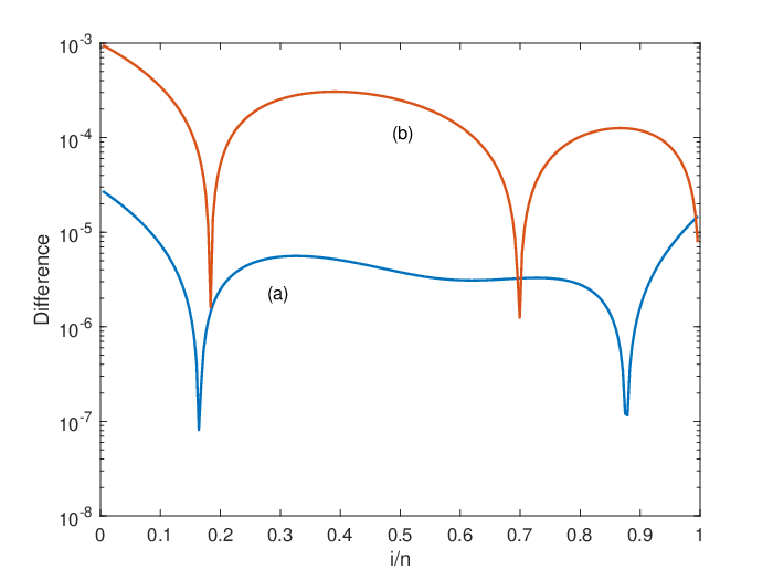
Note that $a$ and $b$ are relatively small terms in (38) for asymptotically large $n$. Figure 3 shows the difference between exact and estimated auto-correlation function $|\rho^{\prime}(i)-\hat{\rho}(i)|$ versus $i/n$ for $n=256$.

As a final proof of the pudding, we compare the (exact) spectrum of full set codewords versus the spectrum, denoted by $H^{\prime}(\omega)$, which is computed using the above approximated auto-correlation function $\rho^{\prime}(i)$. The difference, $H^{\prime}(\omega)/\hat{H}(\omega)$ (dB), between the spectrum, $H^{\prime}(\omega)$, computed using $\rho^{\prime}(i)$, and the exact spectrum, $\hat{H}(\omega)$, of full set codewords, which was computed using generating functions, is plotted in Figure 4. We may observe that the difference between the two spectra is very small, less than 0.05 dB for $n=128$ and less than 0.03 dB for $n=256$.

The LFSW metric, $\chi^{\prime}$ is, using (9),

$$\chi^{\prime}=\frac{1}{12}\sum_{i=1}^{n-1}i^{4}\rho^{\prime}(i)\sim\frac{n^{4}}{720}\left(1+\frac{4}{n}\right).$$

(39)

Table I shows $\chi^{\prime}$ for selected values of $n$, where as a comparison we have listed the LFSW of full set $\text{dc}^{2}$-balanced codes, denoted by $\hat{\chi}$. We may notice that for $n=256$ the difference between $\chi$ and $\hat{\chi}$ is less than half a percent.

In [17], it is postulated that the auto-correlation of $\text{dc}^{2}$-balanced spectral null codes, denoted by $\rho_{a}(i)$, can be modelled by the simple parabola’s equation

$$\rho_{a}(i)=\beta(i+\alpha)(i-n),$$

(40)

where the (real) parameters $\alpha$ and $\beta$ are given by

$$\alpha=-\frac{3n^{2}-2}{5n}$$

and

$$\beta={\frac{-15}{(n-1)(n-2)(4n+3)}}.$$

It has been shown in [17] that the parabola’s equation (40) is an accurate approximation to the exact correlation function of full-set $\text{dc}^{2}$-balanced spectral null codes. Figure 3, Curve (b), shows the difference between exact and estimated auto-correlation function $|\rho_{a}(i)-\hat{\rho}(i)|$ versus $i/n$ for $n=256$. We notice that the newly developed $\rho^{\prime}(i)$, Curve (a), is almost an order more accurate than (40) presented in the prior art. Figure 5, Curve b, shows that the quotient of the exact spectrum and the one based on prior art (40), $\hat{H}(\omega)/H_{a}(\omega)$, is for $n=256$ less than 0.7 dB, and also here we notice that the newly developed theory is more than an order more accurate.

Let the codeword length of a regular full-set dc-balanced code be denoted by $n_{1}$, $n_{1}$ even. Each codeword has an equal number of 0’s and 1’s, so that the number of available dc-balanced codewords, denoted by $N_{\text{dc}}$, is simply [24]

$$N_{\text{dc}}={{n_{1}}\choose{n_{1}/2}}\sim\frac{1}{\sqrt{\frac{\pi}{2}n_{1}}}2^{n_{1}},\,\,n_{1}\gg 1.$$

(41)

The auto-correlation function, $\rho_{1}(i)$, and the spectrum, $H_{1}(\omega)$, of dc-balanced codes is [2]

$$\rho_{1}(i)=\frac{1}{n_{1}(n_{1}-1)}(i-n_{1})$$

(42)

and

$$H_{1}(\omega)={{n_{1}}\over{n_{1}-1}}\left\{1-\left({{{\sin\frac{n_{1}\omega}{2}}}\over{{n_{1}\sin\frac{\omega}{2}}}}\right)^{2}\right\}.$$

(43)

At the very low-frequency end, we have[15]

$$H_{1}(\omega)\sim\chi_{1}\omega^{2},\,\,\omega\ll 1,$$

(44)

where

$$\chi_{1}=\frac{n_{1}(n_{1}+1)}{12}.$$

(45)

We compare the spectral content of dc-balanced versus that of $\text{dc}^{2}$-balanced codes, where we assume that both types of codes have the same redundancy. Let $R$ and $R_{1}$ denote the maximum information rate of a $\text{dc}^{2}$-balanced code or dc-balanced of length $n$ and $n_{1}$, respectively, then we have, using (10),

	$\displaystyle R$	$\displaystyle=$	$\displaystyle\frac{1}{n}\log_{2}N_{\text{dc}^{2}}=\frac{1}{n}\log_{2}\frac{4\sqrt{3}}{\pi n^{2}}2^{n}$		(46)
		$\displaystyle=$	$\displaystyle 1-\frac{1}{n}\log_{2}\frac{\pi n^{2}}{4\sqrt{3}}$

and, using (41),

$$R_{1}=1-\frac{1}{2n_{1}}\log_{2}\frac{\pi}{2}n_{1}.$$

(47)

Table II shows a few examples of the codewords length $n$ and $n_{1}$ for which dc-balanced and $\text{dc}^{2}$-balanced codes have equal redundancy, respectively, that is, $R=R_{1}$. In the range shown in Table II, the codeword length $n$ of a $\text{dc}^{2}$-balanced code is approximately a factor of 4.5 larger than the codeword length $n_{1}$ of a dc-balanced code for achieving the same rate $R=R_{1}$.

Figure 6 shows three examples of spectrum pairs of dc-balanced and $\text{dc}^{2}$-balanced codes with the same redundancy versus frequency for a) $R=R_{1}=0.98$, b) $R=R_{1}=0.94$, and c) $R=R_{1}=0.90$, see also Table II. We may notice the points of intersection of the spectra of dc-balanced and $\text{dc}^{2}$-balanced codes. A further perusal of the diagram reveals that the points of intersection are at around -20 dB, which implies that $\text{dc}^{2}$-balanced codes are to be preferred when a low-frequency spectral suppression is required better than around -20 dB. Additional computations show that this ‘20 dB rule’ applies to all codes with a rate larger than 0.75.

References

- [1] K. W. Cattermole, “Principles of Digital Line Coding,” Int. Journal of Electronics, vol. 55, pp. 3-33, July 1983.
- [2] J. N. Franklin and J. R. Pierce, “Spectra and Efficiency of Binary Codes without DC,” IEEE Trans. Commun., vol. COM-20, pp. 1182-1184, Dec. 1972.
- [3] Y. Ng, K. Cai, K. S. Chan, M. R. Elidrissi, M. Y. Lin, Z. Yuan, C .L. Ong, and S. Ang, “Signal Processing for Dedicated Servo Recording System,” IEEE Trans. Magn., vol. 51, no. 10, Oct. 2015.
- [4] K. Cai, K. A. S. Immink, M. Zhang, and R. Zhao, “Design of Spectrum Shaping Codes for High-Density Data Storage,” Trans. on Consumer Electronics, vol. CE-63, pp. 477-482, Nov. 2017.
- [5] K. A. S. Immink, “Spectral Null Codes,” IEEE Trans. Magn., vol. MAG-26, no. 2, pp. 1130-1135, March 1990.
- [6] A. R. Ndjiongue, H. C. Ferreira, and T. M. N. Ngatched, Visible Light Communications (VLC) Technology, Wiley Encyclopedia of Electrical and Electronics Engineering, 2015.
- [7] M. Oh, “A Flicker Mitigation Modulation Scheme for Visible Light Communications”, 2013 15th International Conference on Advanced Communications Technology (ICACT), PyeongChang, South Korea, Jan. 2013.
- [8] S. Rajagopal, R. D. Roberts, and S-K. Lim, “IEEE 802.15.7 Visible Light Communication: Modulation Schemes and Dimming Support,” IEEE Communications Magazine, vol. 50, No.3, pp. 72-82, March 2012.
- [9] Z. Wang, Q. Wang, W. Huang, and Z. Xu, Visible Light Communications: Modulation and Signal Processing, Wiley-IEEE Press, Jan 2018.
- [10] K. A. S. Immink and G. F. M. Beenker, “Binary Transmission Codes with Higher Order Spectral Zeros at Zero Frequency,” IEEE Trans. Inform. Theory, vol. IT-33, no. 3, pp. 452-454, May 1987.
- [11] L. G. Tallini and B. Bose, “On Efficient High-Order Spectral-Null Codes,” IEEE Trans. Inform. Theory, vol. IT-45, no. 7, pp. 2594-2601, Nov. 1999.
- [12] Y. Xin and I. J. Fair, “Algorithms to Enumerate Codewords for -constrained Channels,” IEEE Trans. Inform. Theory, vol. IT-47, no. 7, pp. 3020-3025, Nov. 2001.
- [13] C. N. Yang, “Efficient Encoding Algorithm for Second-Order Spectral-Null Codes Using Cyclic Bit Shift,” IEEE Transactions on Computers, vol. 57, no. 7, pp. 876-888, July 2008.
- [14] V. Skachek, T. Etzion, and R. M. Roth, “Efficient Encoding Algorithm for Third-order Spectral-Null Codes,” IEEE Trans. Inform. Theory, vol. IT-44, pp. 846-851, March 1998.
- [15] Y. Xin and I. J. Fair, “A Performance Metric for Codes with a High-Order Spectral Null at Zero Frequency,” IEEE Trans. Inform. Theory, vol. IT-50, no. 2, pp. 385-394, Feb. 2004.
- [16] R. M. Roth, P. H. Siegel, and A. Vardy, “Higher-Order Spectral-Null Codes: Constructions and Bounds,” IEEE Trans. Inform. Theory, vol. IT-40, pp. 1826-1840, Nov. 1994.
- [17] K. A. S. Immink an K. Cai, “Estimated Spectra of Higher-Order Spectral Null Codes,” IEEE Commun. Letters, Oct. 2018.
- [18] B.S. Bosik, “The Spectral Density of a Coded Digital Signal,” Bell Syst. Tech. J., vol. 51, pp. 921-932, April 1972.
- [19] G. L. Pierobon, “Codes for Zero Spectral Density at Zero Frequency,” IEEE Trans. Inform. Theory, vol. IT-30, no. 2, pp. 435-439, March 1984.
- [20] J. Justesen, “Information Rates and Power Spectra of Digital Codes,” IEEE Trans. Inform. Theory, vol. IT-28, no. 3, pp. 457-472, May 1982.
- [21] C. M. Monti and G. L. Pierobon, “Codes with a Multiple Spectral Null at Zero Frequency,” IEEE Trans. Inform. Theory, vol. IT-35, no. 2, pp. 463-472, March 1989.
- [22] H. Prodinger, “On the Number of Partitions of {} into Two Sets of Equal Cardinalities and Equal Sums,” Canad. Math. Bull., vol. 25, no. 2, pp. 238-241, 1982.
- [23] P. Flajolet and R. Sedgewick, Analytic Combinatorics, ISBN 978-0-521-89806-5, Cambridge University Press, 2009.
- [24] K. A. S. Immink and J. H. Weber, “Very Efficient Balanced Codes,” IEEE Journal on Selected Areas of Communications, vol. 28, pp. 188-192, 2010.