An Unsupervised Learning Approach for Data Detection in the Presence of Channel Mismatch and Additive Noise Thanks: Kees A. Schouhamer Immink is with Turing Machines Inc, Willemskade 15d, 3016 DK Rotterdam, The Netherlands. E-mail: immink@turing-machines.com. Thanks: Kui Cai is with Singapore University of Technology and Design (SUTD), 8 Somapah Rd, 487372, Singapore. E-mail: cai_kui@sutd.edu.sg.Thanks: This work is supported by Singapore Agency of Science and Technology (A*Star) PSF research grant and SUTD-ZJU grant ZJURP1500102

The symbols of the received word, $r_{i}$, can be straightforwardly quantized to an integer, $\hat{x}_{i}\in{\cal Q}$, with a conventional fixed threshold detector (FTD), also called symbol-by-symbol detector. The threshold function is denoted by $\hat{x}_{i}=\Phi_{\vartheta}(r_{i})$, $\hat{x}_{i}\in{\cal Q}$, where the threshold vector $\mbox{\boldmath$\vartheta$}=$ $(\vartheta_{0},\ldots,\vartheta_{q-2})$ has $q-1$ (real) elements, called thresholds or threshold levels. The threshold vector satisfies the order

The quantization function, $\Phi_{\vartheta}(u)$, of the threshold detector is defined by

For a fixed threshold detector the $q-1$ detection thresholds values, $\vartheta_{i}$, are equidistant at the levels

Threshold detection is very attractive for its implementation simplicity. However, the error performance seriously degrades in the face of channel mismatch [11]. A detector that dynamically adjusts the thresholds is an alternative that offers solace in the face of channel mismatch. The next subsection describes a typical example.

We assume that the channel model is, see (5), $r_{i}=ax_{i}+b+\nu_{i}$, where the gain, $a>0$, and offset, $b$, are unknown parameters, except for the sign of $a$. In case ${\cal S}={\cal Q}^{n}$, that is all possible codewords are allowed, mismatch immune detection is not possible since such a detector cannot distinguish between the word $\hat{\mbox{\boldmath$x$}}$ and its shifted and scaled version $\hat{\mbox{\boldmath$y$}}=c_{1}\hat{\mbox{\boldmath$x$}}+c_{2}$. A designer must judiciously select codewords from ${\cal Q}^{n}$ given adequate constraints that may enable mismatch immune detection. For example, we select for ${\cal S}$ those codewords where the symbols ‘0’ and ‘$q-1$’ must be both at least once present. For the binary case, $q=2$, this implies a slight redundancy as only the all-1 and all-0 words have to be removed, see Subsection VI-A for details. Then, the detector can straightforwardly estimate the gain and offset by

and

where $\hat{a}$ and $\hat{b}$ denote the estimates of the actual channel gain and offset [13]. The dynamic thresholds, denoted by $\hat{\vartheta}_{i}$, are scaled in a similar fashion as the received codeword, that is,

It has been shown [13] that the min-max detector operates over a large range of unknown parameters $a$ and $b$. However, since the estimates, $\hat{a}$ and $\hat{b}$, are biased, the above dynamic threshold detector loses error performance with respect to the matched case, especially for larger codeword length $n$. The detector complexity scales linearly with $n$ as the principal cost is the finding of the maximum and minimum of the $n$ received symbol values. Alternatively, detection based on the prior art Pearson distance, discussed in the next subsection, improves the error performance, but with mounting hardware requirements.

Immink and Weber [11] advocated the Pearson distance instead of the conventional Euclidean distance for improving the error performance of a mismatched noisy channel. We first define two quantities, namely the vector average of the $n$-vector $z$

and the (unnormalized) vector variance of $z$

The Pearson distance, $\delta_{\text{p}}(\mbox{\boldmath$r$},\hat{\mbox{\boldmath$x$}})$, between the received vector $r$ and a codeword $\hat{\mbox{\boldmath$x$}}\in{\cal S}$ is defined by

where

is the well-known (Pearson) correlation coefficient. It is assumed that both codewords $x$ and $\hat{\mbox{\boldmath$x$}}$ are taken from a judiciously chosen codebook $S$, whose properties are explained in subsection VI-A. The Pearson distance is not a metric in the strict mathematical sense, but in engineering parlance it is still called a ‘distance’ since it provides a useful measure of similarity between vectors. A minimum Pearson distance detector outputs the codeword

It can easily be verified that the minimization of $\delta_{\text{p}}(\mbox{\boldmath$r$},\hat{\mbox{\boldmath$x$}})$, and thus ${\mbox{\boldmath$x$}_{\text{o}}}$, is independent of both $a$ and $b$, so that the detection quality is immune to unknown drift of the quantities $a$ and $b$. The minimization operation (16) requires $|S|$ computations, which is impractical for larger $S$. The number of computations can be reduced to $K$, the number of constant composition codes that constitutes the codebook $S$, given by [14]

For the binary case, $q=2$, we have $K=n-1$, so that the detection algorithm (16) scales linearly with $n$. For the non-binary case, it is hard to compute or simulate the error performance of minimum Pearson distance detection in a relevant range of $q$ and $n$ as the number, $K$, of operations grows rapidly with both $q$ and $n$. For example, for $q=4$ and $n=64$ we have $K=43.680$ comparisons (16) per decoded codeword.

The three prior art detection methods discussed above have drawbacks in error performance and/or complexity, and to alleviate these drawbacks, viable alternatives are sought for. In the next section, we propose and investigate a novel detection method with less complexity requirements, which is based on clustering techniques.

The $k$-means clustering technique aims to partition the $n$ received symbols into $k$ sets $V=\{V_{0},V_{1},\ldots,V_{k-1}\}$ so as to minimize the within-cluster sum of squares defined by

where the centroid $\mu_{i}$ is the mean of the received symbols in cluster $V_{i}$, or

The problem of choosing the correct number of clusters is hard, and numerous prior art publications are available to facilitate this choice [2], [3]. Here we assume that a cluster is associated with one of the $k$ symbol values, that is $k=q$.

The $k$-means clustering algorithm is an iteration process that finds a solution of (18). The initial sets $V^{(1)}_{i}$, $0\leq i\leq k-1$, are empty. The superscript integer in parentheses, $(t)$, denotes the iteration tally. We initialize the $k$ centroids $\mu^{(1)}_{i}$, $0\leq i\leq k-1$, by a reasonable choice. For example, Forgy’s method [15] randomly chooses $k$ symbols (assuming $k<n$), $r_{i}$, from the received vector $r$, and uses these as the initial centroids $\mu^{(1)}_{i}$, $1\leq i\leq k$. The choice of the initial centroids has a significant bearing on the error performance of the clustering detection technique. We do not follow Forgy’s approach, and try, dependent on the specific situation at hand, to develop more suitable initial centroids $\mu^{(1)}_{i}$’s. We assume that we order the centroids such that

After the initialization step, we iterate the next two steps until the symbol assignments no longer change.

• •

  Assignment step: Assign the $n$ received symbols, $r_{i}$, to the $k$ sets $V^{(t+1)}_{j}$. If $r_{i}$, $1\leq i\leq n$, is closest to $\mu^{(t)}_{\ell}$, or

  $$\ell=\argmin_{j}\left(r_{i}-\mu^{(t)}_{j}\right)^{2},$$

  (21)

  then $r_{i}$ is assigned to $V^{(t+1)}_{\ell}$. The (temporary) decoded codeword, denoted by

  $$\hat{\mbox{\boldmath$x$}}^{(t)}=(\hat{x}^{(t)}_{1},\ldots,\hat{x}_{n}^{(t)}),$$

  (22)

  is found by

  $$\hat{x}_{i}^{(t)}=\phi_{V^{(t)}}(r_{i}),\,\,1\leq i\leq n,$$

  (23)

  where $\phi_{V^{(t)}}(r_{i})=j$ such that $r_{i}\in V_{j}^{(t)}$.

• •

  Updating step: Compute updated versions of the $k$ means $\mu^{(t+1)}_{j},j\in{\cal Q}$. An update of the new means $\mu^{(t+1)}_{j}$ is found by

  $$\mu^{(t+1)}_{j}=\frac{1}{|V^{(t+1)}_{j}|}\sum_{r_{i}\in V^{(t+1)}_{j}}r_{i},\,\,j\in{\cal Q},$$

  (24)

  where it is understood that if $|V^{(t+1)}_{j}|=0$ that $\mu^{(t+1)}_{j}=\mu^{(t)}_{j}$ (that is, no update).

After running the above routine until the temporary decoded word is unchanged, say at iteration step, $t=t_{o}$, we have $\hat{\mbox{\boldmath$x$}}^{(t_{o}-1)}=\hat{\mbox{\boldmath$x$}}^{(t_{o})}$. Then we have found the final estimate of the sent codeword, $\mbox{\boldmath$x$}_{o}=\hat{\mbox{\boldmath$x$}}^{(t_{o})}$. Bottou [16] showed that the $k$-means cluster algorithm always converges to a simple steady state, and limit cycles do not occur. It is possible, however, that the process reaches a local minimum of the within-cluster sum of squares (18).

We take a closer look at the assignment step of the $k$-means clustering technique, given by (21). Considering the order (20) of the centroids $\mu^{(t)}_{j}$, we simply infer that the symbol $r_{i}$ lies between, say, $\mu^{(t)}_{u}\leq r_{i}\leq\mu^{(t)}_{u+1}$, $0\leq u\leq q-2$. Thus

As

we obtain

Using (7), we yield

where the threshold vector, $\hat{\mbox{\boldmath$\vartheta$}}$, is given by

and the intermediate decoded vector, $\hat{\mbox{\boldmath$x$}}^{(t)}$, is given by

We conclude that the $k$-means cluster detection method is a dynamic threshold detector, where at each update the threshold vector, $\hat{\mbox{\boldmath$\vartheta$}}$, is updated with the means of the members of each cluster using (24).

In the next section, we report on outcomes of computer simulations using channel model (3).

We investigate the error performance of channel model (3), where we assume that the stochastic deviations from the means, $b_{i}$, $i\in{\cal Q}$, are taken from a zero-mean continuous uniform distribution with variance $\sigma^{2}_{b}$. Thus, the $b_{i}$’s lie within the range $-\sqrt{3}\sigma_{b}\leq b_{i}\leq\sqrt{3}\sigma_{b}$. We assume a uniform distribution to guarantee premise (2).

We simply initialize the centroids by $\mu^{(1)}_{i}=i$, $i\in{\cal Q}$, and iterate the assignment and updating steps as outlined above. Figure 1 shows outcomes of computer simulations for the case $n=64$ and $q=4$, where we compare the word error rate (WER) of conventional fixed threshold detection and the novel dynamic threshold detection based on $k$-means clustering classification versus the signal-to-noise ratio (SNR) defined by $=-20\log\sigma$. We plotted two cases, namely $\sigma_{b}=0$ (ideal channel) and $\sigma_{b}=0.1$. As a further comparison we plotted the upper bound of the word error rate of a threshold detector for an ideal additive noise channel, given by [11]

We infer that in case the channel is ideal, $\sigma_{b}=0$, that the error performance of $k$-means clustering detection is close to the performance of both theory and simulation practice of conventional fixed threshold detection. In case the channel is not ideal, $\sigma_{b}=0.1$, $k$-means clustering detection is superior to fixed threshold detection.

The number of iterations, which is an important (time) complexity issue, depends on the integers $q$, $n$, and the signal-to-noise ratio, SNR. The convergence of the iteration process is guaranteed [16], but the speed of convergence is an open question that we studied by computer simulations.

Table I shows results of simulations for the case $q=4$, $n=64$, and $\sigma_{b}=0.1$ (same parameters as used in the simulations depicted in Figure 1). At an SNR = 17 dB, around $91\%$ of the received words is detected without further iterations. In $8\%$ of the detected words, only one iteration of the threshold levels is needed. At an SNR = 20 dB, we found that all but no iterations are required. Thus, since in the large majority of cases no iterations are needed, we conclude that at the cost of a slight additional (time) complexity, the proposed $k$-means clustering classification outperforms fixed threshold detection.

In order to cope with larger uncertainties of both parameters $a$ and $b$, we face an ambiguity problem. For example, let $q=5$, and let $(2,4,4)$ be the received vector. Clearly, it is impossible to distinguish between the two choices, where the sent codeword is $(2,4,4)$ and $a=1$ or where $(1,2,2)$ and $a=2$. Let ${\cal S}$ be the adopted codebook, then we can cope with the above ambiguity if $(2,4,4)\in{\cal S}$ then $(1,2,2)\notin{\cal S}$, or vice versa. The name Pearson code was coined for a set of codewords that can be uniquely decoded by a detector immune to large uncertainties in both $a>0$ and $b$ [13]. Codewords in a Pearson code, ${\cal S}$, satisfy two conditions, namely

• •

  Property A: If $\mbox{\boldmath$x$}\in{\cal S}$ then $c_{1}+c_{2}\mbox{\boldmath$x$}\notin{\cal S}$ for all $c_{1},c_{2}\in\mathbb{R}$ with $(c_{1},c_{2})\neq(0,1)$ and $c_{2}>0$.

• •

  Property B: $\mbox{\boldmath$x$}=(c,c,\ldots,c)\notin{\cal S}$ for all $c\in\mathbb{R}$.

We adopt a Pearson code that has codewords with at least one ‘0’ symbol and at least one ‘$q-1$’ symbol. We may easily verify that such codewords satisfy Properties A and B. The number of allowable $n$-symbol codewords equals [13]

For the binary case, $q=2$, we simply find that

(both the all-‘1’ and all-‘0’ words are deleted).

Here it is assumed that the parameters $a$ and $b$ are completely unknown, except for the sign of $a$, $a>0$. Due to the large uncertainty, we cannot adopt the elementary choice of the initial values of the centroids $\mu^{(1)}_{i}$ as described in Section IV. We propose, following the min-max detector technique described in Subsection III-B, the choice of the initial centroids $\mu^{(1)}_{i}$’s using the minimum, $\min_{i}r_{i}$, and maximum value, $\max_{i}r_{i}$, of the received symbols. The Pearson code guarantees at least one ‘0’ symbol and also at least one ‘$q-1$’ symbol in a codeword. The detector may therefore use the minimum and maximum value of the received symbols as anchor points defining the range of values of the symbols in the received vector. To that end, let

The $q$ initial centroids, $\mu^{(1)}_{i}$, are found by the interpolation

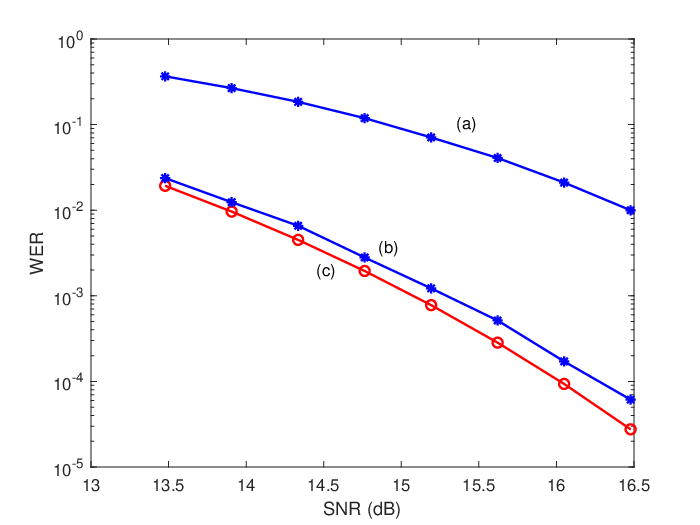
Note that the above initialization step of the modified $k$-means clustering technique has the same effect as the scaling used in the min-max detector (11). Figure 3 shows results of computer simulations for the case $q=4$ and $n=64$ and a gain $a=1.5$. For normalization purposes, we define the SNR by ${\rm SNR}=-20\log(\sigma/a)$. We compared prior art DTD with the $k$-means clustering detection algorithm. The detector based on $k$-means clustering outperforms the prior art min-max detector.

In the next subsection, we discuss a second modification to the basic $k$-means clustering method using regression analysis.

We adopt a second modification to the clustering algorithm of Section IV. In the basic updating step (24), the $k$ clusters centroids are updated by computing a new mean of the members in that cluster only. Here we assume that the linear channel model, $r_{i}=ax_{i}+b+\nu_{i}$, described by (5) holds. We have investigated an alternative method for updating the centroids, $\mu^{(t+1)}_{j}$, by applying the well-known linear regression model [17] that estimates the two coefficients $a$ and $b$ instead of the $q$ centroids $\mu_{i}$.

We start and initialize as described in the previous subsection, where the $q$ initial centroids, $\mu^{(1)}_{i}$, are found by the interpolation

where, as in (34),

For the offset only case, $a$=1, we have

After the initialization, we iterate the next two steps until equilibrium is reached.

• •

  Assignment step: Assign the $n$ received symbols, $r_{i}$, to the $k$ sets $V^{(t+1)}_{j}$. If $r_{i}$, $1\leq i\leq n$, is closest to $\mu^{(t)}_{\ell}$, or

  $$\ell=\argmin_{j}\left(r_{i}-\mu^{(t)}_{j}\right)^{2},$$

  (39)

  then $r_{i}$ is assigned to $V^{(t+1)}_{\ell}$. The (temporary) decoded codeword, denoted by

  $$\hat{\mbox{\boldmath$x$}}^{(t)}=(\hat{x}^{(t)}_{1},\ldots,\hat{x}_{n}^{(t)}),$$

  (40)

  is found by

  $$\hat{x}_{i}^{(t)}=\phi_{V^{(t)}}(r_{i}),\,\,1\leq i\leq n,$$

  (41)

  where $\phi_{V^{(t)}}(r_{i})=j$ such that $r_{i}\in V_{j}^{(t)}$.

• •

  Updating step: Updates of the means $\mu^{(t+1)}_{j},j\in{\cal Q}$ are found by a linear regression model that estimates the coefficients $a$ and $b$. To that end, define the linear regression model

  $$\hat{r}_{i}=\hat{a}^{(t)}\hat{x}_{i}^{(t)}+\hat{b}^{(t)},$$

  (42)

  where the (real-valued) regression coefficients $\hat{a}^{(t)}$ and $\hat{b}^{(t)}$, chosen to minimize $\sum_{i=1}^{n}(r_{i}-\hat{r}_{i})^{2}$, denote the estimates of the unknown quantities $a$ and $b$. The regression coefficients $\hat{a}^{(t)}$ and $\hat{b}^{(t)}$ are found by invoking the well-known linear regression method [17], and we find using (13) and (15)

  $$\hat{a}^{(t)}=\frac{\sum_{i=1}^{n}(r_{i}-\overline{r})(\hat{x}_{i}-\overline{\hat{x}})}{\sum_{i=1}^{n}(\hat{x}_{i}-\overline{\hat{x}})^{2}}=\frac{\sigma_{r}}{\sigma_{\hat{x}^{(t)}}}\rho_{\mbox{\boldmath$r$},\hat{\mbox{\boldmath$x$}}^{(t)}}$$

  (43)

  and

  $$\hat{b}^{(t)}=\overline{r}-\hat{a}^{(t)}\overline{\hat{x}^{(t)}}.$$

  (44)

  We note that for all $\mbox{\boldmath$x$}\in S$, $\sigma_{\hat{x}^{(t)}}\neq 0$ since Property B holds, see Subsection VI-A. The updated $\mu^{(t+1)}_{i}$, $i=0,\ldots,q-1$, are found by the interpolation

  $$\mu^{(t+1)}_{i}=\hat{a}^{(t)}i+\hat{b}^{(t)}.$$

  (45)

  For the offset-only case, $a=1$, we simply find

  $$\hat{b}^{(t)}=\overline{r}-\overline{\hat{x}^{(t)}},$$

  (46)

  and

  $$\mu^{(t+1)}_{i}=i+\hat{b}^{(t)}=i+\overline{r}-\overline{\hat{x}^{(t)}}.$$

  (47)

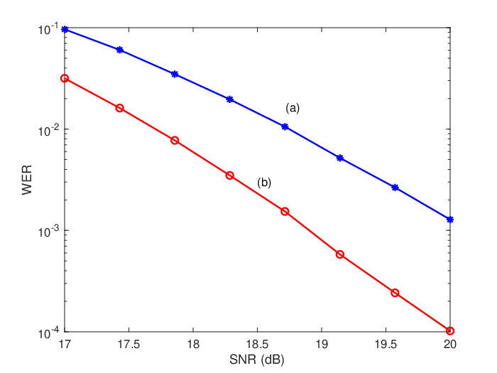
We have conducted a myriad of computer simulations with the above algorithms. Figure 4 compares the error performance of the revised $k$-means clustering using min-max initialization versus the revised $k$-means clustering using regression analysis for the case $q=16$ and $n=64$. The performance difference between the two cluster methods is independent of the unknown quantities $a$ and $b$.

References

- [1] I. Goodfellow, Y. Bengio, and A. Courville, Deep Learning, MIT Press, 2016.
- [2] R. Tibshirani, G. Walther, and T. Hastie, “Estimating the number of clusters in a data set via the gap statistic,” Journal of the Royal Statistical Society, vol. 63, pp. 411-423, 2001.
- [3] A. D. Gordon, Classifcation, 2nd edn., London: Chapman and Hall-CRC, 1999.
- [4] K. A. S. Immink, “A Survey of Codes for Optical Disk Recording,” IEEE J. Select. Areas Commun., vol. 19, no. 4, pp. 756-764, April 2001.
- [5] K. A. S. Immink, “Coding Schemes for Multi-Level Channels with Unknown Gain and/or Offset Using Balance and Energy constraints,” pp. 709-713, IEEE International Symposium on Information Theory, (ISIT), Istanbul, July 2013.
- [6] H. Zhou, A. Jiang, and J. Bruck, “Balanced Modulation for Nonvolatile Memories,” arXiv:1209.0744, Sept. 2012.
- [7] B. Peleato, R. Agarwal, J. M. Cioffi, M. Qin, Member, and P. H. Siegel, “Adaptive Read Thresholds for NAND Flash,” IEEE Transactions on Commun., vol. COM-63, pp. 3069-3081, Sept. 2015.
- [8] F. Sala, R. Gabrys, and L. Dolecek, “Dynamic Threshold Schemes for Multi-Level Non-Volatile Memories,” IEEE Trans. on Commun., pp. 2624-2634, vol. COM-61, July 2013.
- [9] K. A. S. Immink and K. Cai, “Composition Check Codes,” IEEE Trans. Inform. Theory, vol. IT-64, pp. 249-256, Jan. 2018.
- [10] D. Slepian, “Permutation Modulation,” Proc. IEEE, vol. 53, pp. 228-236, March 1965.
- [11] K. A. S. Immink and J. H. Weber, “Minimum Pearson Distance Detection for Multi-Level Channels with Gain and/or Offset Mismatch,” IEEE Trans. Inform. Theory, vol. IT-60, pp. 5966-5974, Oct. 2014.
- [12] K. A. S. Immink, K. Cai, and J. H. Weber, “Dynamic Threshold Detection Based on Pearson Distance Detection,” IEEE Trans. Commun., vol. COM-66, Issue 7, pp. 2958-2965, 2018.
- [13] K. A. S. Immink, “Coding Schemes for Multi-Level Flash Memories that are Intrinsically Resistant Against Unknown Gain and/or Offset Using Reference Symbols,” Electronics Letters, vol. 50, pp. 20-22, 2014.
- [14] K. A. S. Immink and K. Cai, “Design of Capacity-Approaching Constrained Codes for DNA-based Storage Systems,” IEEE Commun. Letters, vol. 22, pp. 224-227, Feb. 2018.
- [15] E. W. Forgy, “Cluster analysis of multivariate data: efficiency versus interpretability of classifications,” Biometrics, vol. 21, pp. 768-769, (1965).
- [16] L. Bottou and Y. Bengio, “Convergence properties of the k-mean algorithms,” Advances in Neural Information Processing Systems 7, pp. 585-592, MIT Press, 1995.
- [17] R. V. Hogg and A. T. Craig, Introduction to Mathematical Statistics, 5th ed. New York: Macmillan, 1995.