Isotonic Regression in Multi-Dimensional Spaces and Graphs

Hang Deng Cun-Hui Zhang^??

In this paper we study minimax and adaptation rates in general isotonic regression. For uniform deterministic and random designs in $[0,1]^{d}$ with $d\geq 2$ and $N(0,1)$ noise, the minimax rate for the $\ell_{2}$ risk is known to be bounded from below by $n^{-1/d}$ when the unknown mean function $f$ is non-decreasing and its range is bounded by a constant, while the least squares estimator (LSE) is known to nearly achieve the minimax rate up to a factor $(\log n)^{\gamma}$ where $n$ is the sample size, $\gamma=4$ in the lattice design and $\gamma=\max\{9/2,(d^{2}+d+1)/2\}$ in the random design. Moreover, the LSE is known to achieve the adaptation rate $(K/n)^{-2/d}\{1\vee\log(n/K)\}^{2\gamma}$ when $f$ is piecewise constant on $K$ hyper-rectangles in a partition of $[0,1]^{d}$ .

Due to the minimax theorem, the LSE is identical on every design point to both the max-min and min-max estimators over all upper and lower sets containing the design point. This motivates our consideration of estimators which lie in-between the max-min and min-max estimators over possibly smaller classes of upper and lower sets, including a subclass of block estimators. Under a $q$ -th moment condition on the noise, we develop $\ell_{q}$ risk bounds for such general estimators for isotonic regression on graphs. For uniform deterministic and random designs in $[0,1]^{d}$ with $d\geq 3$ , our $\ell_{2}$ risk bound for the block estimator matches the minimax rate $n^{-1/d}$ when the range of $f$ is bounded and achieves the near parametric adaptation rate $(K/n)\{1\vee\log(n/K)\}^{d}$ when $f$ is $K$ -piecewise constant. Furthermore, the block estimator possesses the following oracle property in variable selection: When $f$ depends on only a subset $S$ of variables, the $\ell_{2}$ risk of the block estimator automatically achieves up to a poly-logarithmic factor the minimax rate based on the oracular knowledge of $S$ .

, and

Department of Statistics, Rutger University

Keywords: Isotonic regression, multiple isotonic regression, isotonic regression on graphs, max-min estimator, min-max estimator, block estimator, lattice design, random design, minimax rate, adaptive estimation, variable selection, oracle property.

1 Introduction

Let $G=(V,E)$ be a directed graph with vertex set $V$ and edge set $E$ . For $\boldsymbol{a}$ and $\boldsymbol{b}$ in $V$ , we say that $\boldsymbol{a}$ is a descendant of $\boldsymbol{b}$ if $E$ contains a chain of edges from $\boldsymbol{v}_{j}$ to $\boldsymbol{v}_{j+1}$ such that $\boldsymbol{b}=\boldsymbol{v}_{0}$ and $\boldsymbol{a}=\boldsymbol{v}_{m}$ for some finite $m\geq 0$ . We write $\boldsymbol{a}\preceq\boldsymbol{b}$ if $\boldsymbol{a}=\boldsymbol{b}$ or $\boldsymbol{a}$ is a descendant of $\boldsymbol{b}$ . A function $f:V\to{{\mathbb{R}}}$ is non-decreasing on the graph $G$ if $f(\boldsymbol{a})\leq f(\boldsymbol{b})$ whenever $\boldsymbol{a}\preceq\boldsymbol{b}$ . Let ${\mathscr{F}}$ be the class of all non-decreasing functions on $G$ . In isotonic regression, we observe $\boldsymbol{x}_{i}\in V$ and $y_{i}\in{{\mathbb{R}}}$ satisfying

\displaystyle y_{i}=f(\boldsymbol{x}_{i})+\varepsilon_{i},\ i=1,\ldots,n,\ \hbox{for some }f\in{\mathscr{F}},

(1)

where $\varepsilon_{1},\ldots,\varepsilon_{n}$ are independent noise variables with ${\mathbb{E}}\,\varepsilon_{i}=0$ and $\hbox{\rm Var}(\varepsilon_{i})\leq\sigma^{2}$ given the (deterministic or random) design points $\{\boldsymbol{x}_{i}\}$ . Note that we allow $|V|>n$ .

An interesting special case of (1) is the multiple isotonic regression where $V\subset{{\mathbb{R}}}^{d}$ is a subset of a certain Euclidean space of dimension $d$ , and for $\boldsymbol{a}=(a_{1},\ldots,a_{d})^{T}\in{{\mathbb{R}}}^{d}$ and $\boldsymbol{b}=(b_{1},\ldots,b_{d})^{T}\in{{\mathbb{R}}}^{d}$ , $\boldsymbol{a}\preceq\boldsymbol{b}$ iff $a_{j}\leq b_{j}$ for all $1\leq j\leq d$ . In this case, ${\mathscr{F}}$ is the class of all non-decreasing functions on $V$ .

Let $\boldsymbol{f}_{n}=(f(\boldsymbol{x}_{1}),\ldots,f(\boldsymbol{x}_{n}))^{T}$ and ${\widehat{\boldsymbol{f}}}_{n}=(\widehat{f}_{n}(\boldsymbol{x}_{1}),\ldots,\widehat{f}_{n}(\boldsymbol{x}_{n}))^{T}$ for any estimator $\widehat{f}_{n}$ of $f$ . We are interested in the estimation of $f$ under the (normalized) $\ell_{q}$ risk

\displaystyle R_{q}({\widehat{\boldsymbol{f}}}_{n},\boldsymbol{f}_{n})=\frac{1}{n}{\mathbb{E}}\Big\|{\widehat{\boldsymbol{f}}}_{n}-\boldsymbol{f}_{n}\Big\|_{q}^{q}=\frac{1}{n}\sum_{i=1}^{n}{\mathbb{E}}\Big|\widehat{f}_{n}(\boldsymbol{x}_{i})-f(\boldsymbol{x}_{i})\Big|^{q}.

(2)

In this case, a specification of ${\widehat{\boldsymbol{f}}}_{n}$ is sufficient for the definition of $\widehat{f}_{n}$ . For multiple isotonic regression with random design in $V\subseteq{{\mathbb{R}}}^{d}$ , we are also interested in the $L_{q}$ risk

\displaystyle R^{*}_{q}(\widehat{f}_{n},f)={\mathbb{E}}\|\widehat{f}_{n}-f\|_{L_{q}(V)}^{q}={\mathbb{E}}\int_{V}\Big|\widehat{f}_{n}(\boldsymbol{x})-f(\boldsymbol{x})\Big|^{q}d\boldsymbol{x}.

(3)

The literature of univariate isotonic regression ( $d=1$ ) encompasses at least the past six decades; See for example Brunk, 1955, Ayer et al., 1955, Grenander, 1956, Rao, 1969, Groeneboom, 1984, van de Geer, 1990; van de Geer, 1993, Donoho, 1990, Birgé and Massart, 1993, Woodroofe and Sun, 1993, Wang and Chen, 1996, Durot, 2007, Durot, 2008, and Yang and Barber, 2017 among many others for some key developments. The least squares estimator (LSE), say $\widehat{f}_{n}^{(lse)}$ , has been the focus of this literature. We describe in some detail here existing results on minimax and adaptation rates as they are directly related to our study. For any $a<b$ , the $\ell_{q}$ risk of the LSE in the interval $[a,b]$ is bounded by

\displaystyle{\mathbb{E}}\sum_{a\leq x_{i}\leq b}\Big|\widehat{f}_{n}^{(lse)}(x_{i})-f(x_{i})\Big|^{q}\leq C_{q}\sigma^{q}\bigg\{n_{a,b}\bigg(\frac{\Delta_{a,b}(\boldsymbol{f}_{n}/\sigma)}{n_{a,b}}\wedge 1\bigg)^{q/3}+\sum_{j=1}^{n_{a,b}}j^{-q/2}\bigg\},

(4)

where $\Delta_{a,b}(\boldsymbol{f}_{n}/\sigma)=\max_{a\leq x_{i}<x_{j}\leq b}\{f(x_{j})-f(x_{i})\}/\sigma$ is the range-to-noise ratio for the mean vector $\boldsymbol{f}_{n}$ in $[a,b]$ , $n_{a,b}=\#\{j:a\leq x_{j}\leq b\}$ is the number of design points in the interval, and $C_{q}$ is a constant depending on $q$ only. This result can be found in Meyer and Woodroofe, 2000 for $n_{a,b}=n$ , $q=2$ and $\varepsilon_{i}\sim N(0,\sigma^{2})$ , and in Zhang, 2002 for general $a<b$ and $1\leq q<3$ under a $(q\vee 2)$ -th moment condition on $\varepsilon_{i}$ . For $\Delta_{-\infty,\infty}(\boldsymbol{f}_{n}/\sigma)\leq\Delta^{*}_{n}\asymp 1$ , (4) yields the cube-root rate $\sigma^{q}(\Delta^{*}_{n}/n)^{q/3}$ for the LSE in terms of the $\ell_{q}$ risk in (2). By summing over the risk bound (4) over $K$ intervals $[a_{k},b_{k}]$ with $\Delta_{a_{k},b_{k}}(\boldsymbol{f}_{n}/\sigma)=0$ , the LSE can be seen to achieve the near parametric adaptation rate $(K/n)\{1\vee\log(n/K)\}$ in the mean squared risk when the unknown $f$ is piecewise constant on the $K$ intervals and $x_{i}\in\cup_{k=1}^{K}[a_{k},b_{k}]$ for all $i\leq n$ . This adaptation rate was explicitly given in Chatterjee et al., 2015. However, Gao et al., 2017 proved that the sharp adaptation rate in the mean squared risk, achieved by a penalized LSE, is $(K/n)\log\log(16n/K)$ in the piecewise constant case. Moreover, by summing over the risk bound (4) over a growing number of disjoint intervals, the LSE has been shown to converge faster than the cube root rate when the measure $f(dx)$ is singular to the Lebesgue measure (Zhang, 2002).

Compared with the rich literature on univariate isotonic regression, our understanding of the multiple isotonic regression, i.e. $V\subset{{\mathbb{R}}}^{d}$ with $d>1$ , is quite limited. A major difficulty is that the design points are typically only partially ordered. Univariate risk bounds can be directly applied to linearly ordered paths in $V$ , but this typically does not yield a nearly minimax rate. However, significant advances have been made recently on the minimax and adaptation rates for the LSE. For $n_{1}\times\cdots\times n_{d}$ lattice designs with $n=\prod_{j=1}^{d}n_{j}$ , the LSE provides

\displaystyle R_{2}({\widehat{\boldsymbol{f}}}_{n}^{(lse)},\boldsymbol{f}_{n})\leq C_{d}\sigma^{2}\bigg\{\Delta(\boldsymbol{f}_{n}/\sigma)n^{-1/d}(\log n)^{\gamma}+n^{-2/d}(\log n)^{2\gamma}\bigg\}

(5)

in certain settings, where $\Delta(\boldsymbol{f}_{n}/\sigma)=\max_{1\leq i<j\leq n}|f(\boldsymbol{x}_{i})-f(\boldsymbol{x}_{j})|/\sigma$ is the range-to-noise ratio of the mean over the design points. For Gaussian $\varepsilon_{i}$ and $n_{1}=\cdots=n_{d}$ , the minimax rate is bounded from below by

\displaystyle\inf_{{\widehat{\boldsymbol{f}}}_{n}}\sup_{\Delta(\boldsymbol{f}_{n}/\sigma)\leq\Delta^{*}_{n}}R_{2}({\widehat{\boldsymbol{f}}}_{n},\boldsymbol{f}_{n})\geq\sigma^{2}\min\Big\{1,C_{0}n^{-1/d}\Delta^{*}_{n}\Big\}.

(6)

Moreover, when $f$ is piecewise constant on $K$ hyper-rectangles in a partition of the lattice,

\displaystyle R_{2}({\widehat{\boldsymbol{f}}}_{n}^{(lse)},\boldsymbol{f}_{n})\leq C_{d}\sigma^{2}(K/n)^{2/d}\{1\vee\log(n/K)\}^{2\gamma}.

(7)

For $d=2$ and Gaussian noise, Chatterjee et al., 2018 proved the above mean squared risk bounds with $\gamma=4$ . Thus, up to a logarithmic factor, the LSE is nearly rate minimax for a wide range of $\Delta^{*}_{n}$ and also nearly adaptive to the parametric rate $\sigma^{2}K/n$ when $f$ is piecewise constant on $K$ rectangles. Han et al., 2017 extended the results of Chatterjee et al., 2018 from $d=2$ to $d>2$ under the conditions $n_{1}=\cdots=n_{d}$ and $\Delta(\boldsymbol{f}_{n}/\sigma)\leq\Delta^{*}_{n}=1$ in (5) and (6), and also proved parallel results for random designs with a larger $\gamma=\max\{9/2,(d^{2}+d+1)/2\}$ . However, there is still a gap of a poly-logarithmic factor between such upper and lower minimax bounds for $d\geq 2$ , and it is still unclear from (7) the feasibility of near adaptation to the parametric rate $\sigma^{2}K/n$ for $d\geq 3$ when $f$ is piecewise constant on $K$ hyper-rectangles.

We have also seen some progresses in adaptive estimation to variable selection in isotonic regression on lattices with $\max_{j\leq d}n_{j}\leq C_{d}n^{1/d}$ . When the unknown mean function depends on only a known subset of $s$ variables, say $f(\boldsymbol{x})=f_{S}(\boldsymbol{x}_{S})$ where $\boldsymbol{x}_{S}=(x_{j},j\in S)^{T}$ with $|S|=s$ , one may use the LSE, say $\widehat{f}_{n,S}^{(lse)}$ , based on the average of $y_{i}$ given $\boldsymbol{x}_{S}$ to attain

\displaystyle R_{2}({\widehat{\boldsymbol{f}}}_{n,S}^{(lse)},\boldsymbol{f}_{n})\leq\begin{cases}C_{d}\sigma_{S}^{2}\Big[\Delta(\boldsymbol{f}_{n}/\sigma_{S})n^{-1/d}(\log n)^{\gamma}+n^{-2/d}(\log n)^{2\gamma}\Big],&s\geq 2,\cr C_{d}\sigma_{S}^{2}\Big[\{(\Delta(\boldsymbol{f}_{n}/\sigma_{S})n^{-1/d})\wedge 1\}^{2/3}+n^{-1/d}\log n\Big],&s=1,\end{cases}

(8)

with $\sigma_{S}^{2}=\sigma^{2}/\prod_{j\not\in S}n_{j}\leq C_{d}\sigma^{2}/n^{1-s/d}$ , which would match the minimax rate for Gaussian $\varepsilon_{i}$ for a proper range of $\Delta(\boldsymbol{f}_{n}/\sigma_{S})$ as we discussed in the previous paragraph. For unknown $S$ with $d\geq 2$ and $\Delta(\boldsymbol{f}_{n}/\sigma)\leq 1=\sigma$ , Han et al., 2017 proved that the LSE $\widehat{f}_{n}^{(lse)}$ for the general $f$ automatically achieves the rate $n^{-4/(3d)}(\log n)^{16/3}$ for $s=d-1$ and $n^{-2/d}(\log n)^{8}$ for $s\leq d-2$ . As $\Delta(\boldsymbol{f}_{n}/\sigma_{S})\asymp n^{(d-s)/(2d)}$ in their setting, (8) would yield the rates $n^{-(d-s)/(2d)-1/d}$ for $s\geq 2$ and $n^{-(d-1)/d-(3-d)_{+}/(3d)}$ for $s=1$ up to a logarithmic factor. These oracle minimax rates nearly match the adaptation rates in Han et al., 2017 for $d-s=2$ or $(d,s)=(2,1)$ , but not for other configurations of $(d,s)$ .

We consider isotonic regression on directed graphs, i.e. with general domain $V$ in (1), including $V\subset{{\mathbb{R}}}^{d}$ as a special case. In this general setting, Robertson et al., 1988 proved the following minimax formula for the LSE on the design points:

\displaystyle\widehat{f}_{n}^{(lse)}(\boldsymbol{x})=\max_{U\ni\boldsymbol{x}}\min_{L\ni\boldsymbol{x}}{\overline{y}}_{U\cap L}=\min_{L\ni\boldsymbol{x}}\max_{U\ni\boldsymbol{x}}{\overline{y}}_{U\cap L}

(9)

for $\boldsymbol{x}=\boldsymbol{x}_{i}$ , $i=1,\ldots,n$ , where the maximum is taken over all upper sets $U$ containing $\boldsymbol{x}$ , the minimum over all lower sets $L$ containing $\boldsymbol{x}$ , and ${\overline{y}}_{A}$ is the average of the observed $y_{i}$ over $\boldsymbol{x}_{i}\in A$ for any $A\subseteq V$ . As the high complexity of the upper and lower sets for $d\geq 2$ could be the culprit behind the possible suboptimal performance of the LSE in convergence and adaptation rates, we consider a class of block estimators involving rectangular upper and lower sets. As the minimax theorem no longer holds in this setting in general, the block estimator, say $\widehat{f}_{n}^{(block)}(\boldsymbol{x})$ , is defined as any estimator in-between the following max-min and min-max estimators,

	$\displaystyle\widehat{f}_{n}^{(max-min)}(\boldsymbol{x})$	$\displaystyle=$	$\displaystyle\max_{\boldsymbol{u}\preceq\boldsymbol{x},n_{\boldsymbol{u},*}>0}\ \min_{\boldsymbol{x}\preceq\boldsymbol{v},n_{\boldsymbol{u},\boldsymbol{v}}>0}{\overline{y}}_{[\boldsymbol{u},\boldsymbol{v}]},\quad\forall\ \boldsymbol{x}\in V,$		(10)
	$\displaystyle\widehat{f}_{n}^{(min-max)}(\boldsymbol{x})$	$\displaystyle=$	$\displaystyle\min_{\boldsymbol{x}\preceq\boldsymbol{v},n_{*,\boldsymbol{v}}>0}\ \max_{\boldsymbol{u}\preceq\boldsymbol{x},n_{\boldsymbol{u},\boldsymbol{v}}>0}{\overline{y}}_{[\boldsymbol{u},\boldsymbol{v}]},\quad\forall\ \boldsymbol{x}\in V,$		(11)

where $[\boldsymbol{u},\boldsymbol{v}]=\{\boldsymbol{x}:\boldsymbol{u}\preceq\boldsymbol{x}\preceq\boldsymbol{v}\}$ , $n_{\boldsymbol{u},\boldsymbol{v}}=\#\{i\leq n:\boldsymbol{x}_{i}\in[\boldsymbol{u},\boldsymbol{v}]\}$ , $n_{\boldsymbol{u},*}=\#\{i\leq n:\boldsymbol{u}\preceq\boldsymbol{x}_{i}\}$ and $n_{*,\boldsymbol{v}}=\#\{i\leq n:\boldsymbol{x}_{i}\preceq\boldsymbol{v}\}$ . The idea of replacing the general level sets $U\cap L$ by rectangular blocks $[\boldsymbol{u},\boldsymbol{v}]$ is not new as a preliminary version of the block estimator in the case of $V=[0,1]^{d}$ was considered in Fokianos et al., 2017. Some more delicate details of different versions of the block estimator are discussed in Section 2.

We derive in Section 3 a general $\ell_{q}$ risk bound for the above block estimator on graphs. For $n_{1}\times\cdots\times n_{d}$ lattice designs with $d\geq 2$ , our general risk bound yields

\displaystyle R_{2}\Big({\widehat{\boldsymbol{f}}}_{n}^{(block)},\boldsymbol{f}_{n}\Big)\leq C_{d}\sigma^{2}\min\Big\{1,\Delta(\boldsymbol{f}_{n}/\sigma)n^{-1/d}(\log n)^{I\{d=2\}}+n^{-1}(\log n)^{d}\Big\}

(12)

when $\max_{j\leq d}n_{j}\leq C_{d}n^{1/d}$ , compared with (5) and (6), and the adaptation rate

\displaystyle R_{2}\Big({\widehat{\boldsymbol{f}}}_{n}^{(block)},\boldsymbol{f}_{n}\Big)\leq C_{d}\sigma^{2}(K/n)\{1\vee\log(n/K)\}^{d}

(13)

when the true $f$ is non-decreasing and piecewise constant on $K$ hyper-rectangles, compared with (7).

We also explore the phase transition of the risk bounds, both the minimax lower bound and the upper risk bound for the block estimator, by presenting them using its effective dimension $s$ in the sense that the risk bound only depends on the largest $s$ $n_{j}$ ’s. For example, when $n_{1}\geq n_{2}\geq\cdots\geq n_{d}$ and $n_{2}^{3/2}/n_{1}^{1/2}\leq\Delta(\boldsymbol{f}_{n}/\sigma)$ , we show that the risk bound for the block estimator in $d$ -dimensional isotonic regression with $n$ design points is almost no different from that in univariate isotonic regression with $n_{1}$ design points. This phase transition, captured by effective dimension, proved for $d=2$ in Chatterjee et al., 2018, is new for $d>2$ .

Moreover, perhaps more interestingly, we prove that when the unknown $f$ depends on an unknown set of $s$ variables, the block estimator achieves near adaptation to the oracle selection in the sense that for $\Delta(\boldsymbol{f}_{n}/\sigma)\leq\Delta^{*}_{n}$ ,

			$\displaystyle R_{2}({\widehat{\boldsymbol{f}}}_{n}^{(block)},\boldsymbol{f}_{n})$		(14)
		$\displaystyle\leq$	$\displaystyle\begin{cases}C_{d}\sigma_{S}^{2}\min\Big[(\log n)^{d-s},\Delta^{}_{n}n^{(d-s-2)/(2d)}(\log n)^{I\{s=2\}}+n^{-s/d}(\log n)^{d}\Big],&s\geq 2,\cr C_{d}\sigma_{S}^{2}\min\Big[(\log n)^{d-1},\big(\Delta^{}_{n}n^{(d-s-2)/(2d)}\big)^{2/3}+n^{-1/d}(\log n)^{d}\Big],&s=1,\end{cases}$		(14)

with $\sigma_{S}^{2}=\sigma^{2}/\prod_{j\not\in S}n_{j}\leq C_{d}\sigma^{2}/n^{1-s/d}$ , while the oracle minimax rate with the knowledge of $S$ is bounded from below by

			$\displaystyle\inf_{{\widehat{\boldsymbol{f}}}_{n}}\sup_{\boldsymbol{f}_{n}}\Big\{R_{2}({\widehat{\boldsymbol{f}}}_{n},\boldsymbol{f}_{n}):\boldsymbol{f}_{n}\in{\mathscr{F}}_{n},\,f(\boldsymbol{x})=f_{S}(\boldsymbol{x}_{S}),\Delta(\boldsymbol{f}_{n}/\sigma)\leq\Delta^{*}_{n}\Big\}$		(15)
		$\displaystyle\geq$	$\displaystyle\begin{cases}C_{d}\sigma^{2}n^{-1+s/d}\min\Big[1,\Delta^{}_{n}n^{(d-s-2)/(2d)}\Big],&s\geq 2,\cr C_{d}\sigma^{2}n^{-1+1/d}\min\Big[1,\big(\Delta^{}_{n}n^{(d-3)/(2d)}\big)^{2/3}\Big],&s=1,\end{cases}$		(15)

where ${\mathscr{F}}_{n}=\{\boldsymbol{f}_{n}:f\in{\mathscr{F}}\}$ .

Let ${\overline{\boldsymbol{f}}}^{*}_{n}$ be the noiseless version of the block estimator. When the isotonic regression model is misspecified in the sense of having a non-monotone regression function, we prove that the error bounds discussed above still hold if ${\overline{\boldsymbol{f}}}^{*}_{n}$ is treated as the estimation target; (12), (13) and (14) are valid with $\boldsymbol{f}_{n}$ replaced by ${\overline{\boldsymbol{f}}}^{*}_{n}$ when $f\not\in{\mathscr{F}}$ in (1). However, such results are of a less ideal form compared with the existing oracle inequalities for the LSE under misspecified monotonicity assumption (Chatterjee et al., 2015; Bellec, 2018; Chatterjee et al., 2018; Han et al., 2017).

We summarize our main results as follows. In terms of the mean squared risk, the block estimator is rate minimax for $\Delta(\boldsymbol{f}_{n}/\sigma)\leq\Delta^{*}_{n}$ with a wide range of $\Delta^{*}_{n}$ (with no extra logarithmic factor for $d\neq 2$ ), achieves near parametric adaptation in the piecewise constant case, and also achieves near adaptation to the oracle minimax rate in variable selection. Furthermore, we prove parallel results for the integrated risk for i.i.d. random designs in $[0,1]^{d}$ when the joint density of the design point is uniformly bounded away from zero and infinity. In addition to Sections 2 and 3, we present in Section 4 some simulation results to demonstrate the advantage of the block estimator over the LSE in multiple isotonic regression. The full proofs of all theorems, propositions and lemmas in this paper are relegated to the supplement (Deng and Zhang, 2019).

Here and in the sequel, the following notation is used. For $\{\boldsymbol{a},\boldsymbol{b}\}\subset V$ , we say $\boldsymbol{b}$ is larger than $\boldsymbol{a}$ when $\boldsymbol{a}\preceq\boldsymbol{b}$ , and we set $[\boldsymbol{a},\boldsymbol{b}]=\{\boldsymbol{x}\in V:\boldsymbol{a}\preceq\boldsymbol{x}\preceq\boldsymbol{b}\}$ as a block in $G=(V,E)$ . We denote by $n_{A}$ the number of sampled points in $A$ , i.e. $n_{A}=\#\{i\leq n:\boldsymbol{x}_{i}\in A\}$ , and set $n_{\boldsymbol{a},\boldsymbol{b}}=n_{[\boldsymbol{a},\boldsymbol{b}]}$ , $n_{\boldsymbol{a},*}=\#\{i\leq n:\boldsymbol{a}\preceq\boldsymbol{x}_{i}\}$ , and $n_{*,\boldsymbol{b}}=\#\{i\leq n:\boldsymbol{x}_{i}\preceq\boldsymbol{b}\}$ . For $\boldsymbol{a}=(a_{1},\ldots,a_{d})^{T}\in{{\mathbb{R}}}^{d}$ and $\boldsymbol{b}=(b_{1},\ldots,b_{d})^{T}\in{{\mathbb{R}}}^{d}$ , $\boldsymbol{a}\preceq\boldsymbol{b}$ iff $a_{j}\leq b_{j}$ for all $1\leq j\leq d$ , and this is also expressed as $\boldsymbol{a}\leq\boldsymbol{b}$ . We denote by $C$ a positive numerical constant, and $C_{\rm index}$ a positive constant depending on the “index” only. For example, $C_{q,d}$ is a positive constant depending on $(q,d)$ only. For the sake of convenience, the value of such a constant with the same subscript may change from one appearance to the next. We may write $x\lesssim_{\rm index}y$ when $x\leq C_{\rm index}\,y$ . Finally, we set $\log_{+}(x)=1\vee\log x$ .

2 The least squares and block estimators

Given design points $\boldsymbol{x}_{i}\in V$ and responses $y_{i}\in{{\mathbb{R}}}$ , the isotonic LSE is formally defined as

\displaystyle\widehat{f}_{n}^{(lse)}=\mathop{\rm arg\,min}_{f\in{\mathscr{F}}}\sum_{i=1}^{n}\big\{y_{i}-f(\boldsymbol{x}_{i})\big\}^{2},

where ${\mathscr{F}}=\{f:f(\boldsymbol{u})\leq f(\boldsymbol{v})\ \forall\ \boldsymbol{u}\preceq\boldsymbol{v}\}$ is the set of all non-decreasing functions on the directed graph $G=(V,E)$ . As the squared loss only involves the value of $f$ at the design points, this LSE is any non-decreasing extension of the LSE of the mean vector $\boldsymbol{f}_{n}=(f(\boldsymbol{x}_{1}),\ldots,f(\boldsymbol{x}_{n}))^{T}$ in (1),

\displaystyle{\widehat{\boldsymbol{f}}}_{n}^{(lse)}=\mathop{\rm arg\,min}_{\boldsymbol{f}_{n}\in{\mathscr{F}}_{n}}\|\boldsymbol{y}-\boldsymbol{f}_{n}\|_{2}^{2},

(16)

where $\boldsymbol{y}=(y_{1},\ldots,y_{n})^{T}$ and ${\mathscr{F}}_{n}=\{\boldsymbol{f}_{n}:f\in{\mathscr{F}}\}\subset{{\mathbb{R}}}^{n}$ . As ${\mathscr{F}}_{n}$ is defined with no more than ${n\choose 2}$ linear constraints, ${\widehat{\boldsymbol{f}}}_{n}^{(lse)}$ can be computed with quadratic programming. Potentially more efficient algorithms for the LSE have been developed in Dykstra, 1983, Kyng et al., 2015 and Stout, 2015, among others.

As mentioned in the introduction, the LSE ${\widehat{\boldsymbol{f}}}_{n}^{(lse)}$ has an explicit representation in the minimax formula (9) for isotonic regression on graphs in general (Robertson et al., 1988), although this fact is better known in the univariate case. As the high complexity of the general upper and lower sets in the minimax formula seems to be the cause of the analytical or possibly real gap between the risk of the LSE and the optimal minimax and adaptation rates, we consider in this paper block estimators $\widehat{f}_{n}^{(block)}$ of the form

	$\displaystyle\min\Big\{\widehat{f}_{n}^{(max-min)}(\boldsymbol{x}),\widehat{f}_{n}^{(min-max)}(\boldsymbol{x})\Big\}$	(17)
$\displaystyle\leq$	$\displaystyle\widehat{f}_{n}^{(block)}(\boldsymbol{x})$	(18)
$\displaystyle\leq$	$\displaystyle\max\Big\{\widehat{f}_{n}^{(max-min)}(\boldsymbol{x}),\widehat{f}_{n}^{(min-max)}(\boldsymbol{x})\Big\},\quad\forall\ \boldsymbol{x}\in V,$	(18)

where $\widehat{f}_{n}^{(max-min)}$ and $\widehat{f}_{n}^{(min-max)}$ are the block max-min and min-max estimators given in (10). It is clear from (10) that both the max-min and min-max estimators are non-decreasing on the graph $G=(V,E)$ as the maximum is taken over increasing classes indexed by $\boldsymbol{x}\in V$ and the minimum over decreasing classes. However, the monotonicity of the block estimator, $\widehat{f}_{n}^{(block)}\in{\mathscr{F}}$ or even ${\widehat{\boldsymbol{f}}}_{n}^{(block)}\in{\mathscr{F}}_{n}$ , is optional in our analysis. A practical monotone solution is

\displaystyle\widehat{f}_{n}^{(block)}(\boldsymbol{x})=\frac{1}{2}\Big\{\widehat{f}_{n}^{(max-min)}(\boldsymbol{x})+\widehat{f}_{n}^{(min-max)}(\boldsymbol{x})\Big\},\quad\forall\boldsymbol{x}\in V.

(19)

We note that the estimator (17) is defined on the entire $V$ . This is needed as we shall consider the $L_{q}$ risk (3) as well as the $\ell_{q}$ risk (2). It would be tempting to define the block estimator by

\displaystyle\max_{\boldsymbol{u}\preceq\boldsymbol{x}}\min_{\boldsymbol{x}\preceq\boldsymbol{v}}{\overline{y}}_{[\boldsymbol{u},\boldsymbol{v}]}\leq\widehat{f}^{(block)}(\boldsymbol{x})\leq\min_{\boldsymbol{x}\preceq\boldsymbol{v}}\max_{\boldsymbol{u}\preceq\boldsymbol{x}}{\overline{y}}_{[\boldsymbol{u},\boldsymbol{v}]}

(Fokianos et al., 2017). However, unfortunately, when $\boldsymbol{x}$ is not a design point, ${\overline{y}}_{[\boldsymbol{u},\boldsymbol{v}]}$ is undefined when $[\boldsymbol{u},\boldsymbol{v}]$ contains no data point, and $\widehat{f}_{n}^{(max-min)}(\boldsymbol{x})\leq\widehat{f}_{n}^{(min-max)}(\boldsymbol{x})$ is not guaranteed to hold even for properly defined max-min and min-max estimators in (10), even in the univariate case. For example, for $V=[0,1]$ with two data points $(x_{1},y_{1})=(0,1)$ and $(x_{2},y_{2})=(1,2)$ , (10) gives $\widehat{f}_{n}^{(max-min)}(0.5)=2>1=\widehat{f}_{n}^{(min-max)}(0.5)$ . We do have

\displaystyle\widehat{f}_{n}^{(max-min)}(\boldsymbol{x}_{i})\leq\widehat{f}_{n}^{(min-max)}(\boldsymbol{x}_{i}),\quad i=1,\ldots,n,

(20)

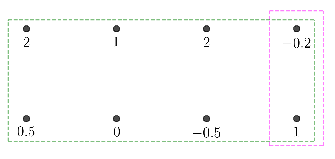
but the minimax formula $\widehat{f}_{n}^{(max-min)}=\widehat{f}_{n}^{(min-max)}$ may fail even on the design points as the example in Figure 1 demonstrates.

Refer to caption — Fig 1: Responses $y_{i}$ on a $4\times 2$ lattice design: At design point $\boldsymbol{x}=(4,1)$ , $\widehat{f}_{n}^{(max-min)}(\boldsymbol{x})=0.4$ is attained by the mean inside the magenta box and $\widehat{f}_{n}^{(min-max)}(\boldsymbol{x})=0.725$ attained by the mean inside the green box.

In the rest of this section, we prove that the max-min and min-max estimators defined with upper and lower sets in a graph $G$ , including the LSE, can always be expressed as the block estimators defined as in (17) but over a larger graph than $G$ , so that our analysis of general block estimators is also relevant to the LSE. We present our argument in a more general setting as follows.

Formally, a subset of vertices $U\subseteq V$ is called an upper set if $U=\{\boldsymbol{x}:f(\boldsymbol{x})>t\}$ for some $f\in{\mathscr{F}}$ and real $t$ , or equivalently the indicator function $1_{U}$ is non-decreasing on $G$ , i.e. $1_{U}\in{\mathscr{F}}$ ; a subset $L\subseteq V$ is called a lower set if $L=\{\boldsymbol{x}:f(\boldsymbol{x})\leq t\}$ for some $f\in{\mathscr{F}}$ and $t\in{{\mathbb{R}}}$ , i.e. the complement of an upper set. Let ${\mathscr{U}}$ be the collection of all upper sets, ${\mathscr{L}}$ the collection of all lower sets, and

\displaystyle{\mathscr{U}}_{\boldsymbol{x}}\subseteq\{U\in{\mathscr{U}}:\boldsymbol{x}\in U\}\ \hbox{ and }\ {\mathscr{L}}_{\boldsymbol{x}}\subseteq\{L\in{\mathscr{L}}:\boldsymbol{x}\in L\}

be certain subsets of the collections of upper and lower sets containing $\boldsymbol{x}$ . The max-min and min-max estimator can be defined in general as

	$\displaystyle\widehat{f}_{n}^{(max-min)}(\boldsymbol{x})$	$\displaystyle=$	$\displaystyle\max_{U\in{\mathscr{U}}_{\boldsymbol{x}},n_{U}>0}\min_{L\in{\mathscr{L}}_{\boldsymbol{x}},n_{U\cap L}>0}{\overline{y}}_{U\cap L},\quad\boldsymbol{x}\in V,$		(21)
	$\displaystyle\widehat{f}_{n}^{(min-max)}(\boldsymbol{x})$	$\displaystyle=$	$\displaystyle\min_{L\in{\mathscr{L}}_{\boldsymbol{x}},n_{L}>0}\max_{U\in{\mathscr{U}}_{\boldsymbol{x}},n_{U\cap L}>0}{\overline{y}}_{U\cap L},\quad\boldsymbol{x}\in V,$		(22)

where $n_{A}=\{i\leq n:\boldsymbol{x}_{i}\in A\}$ . These max-min and min-max estimators are non-decreasing in $\boldsymbol{x}$ on the entire graph if ${\mathscr{U}}_{\boldsymbol{x}}$ is non-decreasing in $\boldsymbol{x}$ and ${\mathscr{L}}_{\boldsymbol{x}}$ non-increasing in $\boldsymbol{x}$ : ${\mathscr{U}}_{\boldsymbol{x}}\subseteq{\mathscr{U}}_{\boldsymbol{x}^{\prime}}$ and ${\mathscr{L}}_{\boldsymbol{x}}\supseteq{\mathscr{L}}_{\boldsymbol{x}^{\prime}}$ for all ordered pairs $\boldsymbol{x}\preceq\boldsymbol{x}^{\prime}$ .

By (9), the LSE is a special case of (21) when ${\mathscr{U}}_{\boldsymbol{x}}$ and ${\mathscr{L}}_{\boldsymbol{x}}$ are taken to be the largest possible. The block max-min and min-max estimators (10) are special cases of (21) with ${\mathscr{U}}_{\boldsymbol{x}}=\{[\boldsymbol{u},*]:\boldsymbol{u}\preceq\boldsymbol{x}\}$ and ${\mathscr{L}}_{\boldsymbol{x}}=\{[*,\boldsymbol{v}]:\boldsymbol{x}\preceq\boldsymbol{v}\}$ . Conversely, the LSE, and more generally (21), can be written as

	$\displaystyle\widehat{f}_{n}^{(max-min)}(\boldsymbol{x})$	$\displaystyle=$	$\displaystyle\max_{\boldsymbol{u}\in A_{\boldsymbol{x}},n_{\boldsymbol{u},*}>0}\min_{\boldsymbol{v}\in B_{\boldsymbol{x}},n_{\boldsymbol{u},\boldsymbol{v}}>0}{\overline{y}}_{[\boldsymbol{u},\boldsymbol{v}]},\quad\boldsymbol{x}\in V,$		(23)
	$\displaystyle\widehat{f}_{n}^{(min-max)}(\boldsymbol{x})$	$\displaystyle=$	$\displaystyle\min_{\boldsymbol{v}\in B_{\boldsymbol{x}},n_{*,\boldsymbol{v}}>0}\max_{\boldsymbol{u}\in A_{\boldsymbol{x}},n_{\boldsymbol{u},\boldsymbol{v}}>0}{\overline{y}}_{[\boldsymbol{u},\boldsymbol{v}]},\quad\boldsymbol{x}\in V,$		(24)

based on the average response in blocks $[\boldsymbol{u},\boldsymbol{v}]$ for suitable $A_{\boldsymbol{x}}$ and $B_{\boldsymbol{x}}$ in a larger graph $G^{*}$ in which $G$ is a subgraph. We define $G^{*}$ by amending $G$ with new nodes and edges as follows. For each upper set $U$ , we amend $G$ with node $\boldsymbol{u}^{(new)}=\boldsymbol{u}^{(new,U)}$ and edges $\{\boldsymbol{u}\to\boldsymbol{u}^{(new)}:\boldsymbol{u}\in U\}$ , whereas for each lower set $L$ , we amend $G$ with node $\boldsymbol{v}^{(new)}=\boldsymbol{v}^{(new,L)}$ and edges $\{\boldsymbol{v}^{(new)}\to\boldsymbol{v}:\boldsymbol{v}\in L\}$ . Define in the new graph $G^{*}$ the estimators (23) with $A_{\boldsymbol{x}}=\{\boldsymbol{u}^{(new,U)}:U\in{\mathscr{U}}_{\boldsymbol{x}}\}$ and $B_{\boldsymbol{x}}=\{\boldsymbol{v}^{(new,L)}:L\in{\mathscr{L}}_{\boldsymbol{x}}\}$ . Then, the restriction of (23) on $G$ is identical to (21) as $[\boldsymbol{u}^{(new,U)},\boldsymbol{v}^{(new,L)}]$ contains the same set of design points as $U\cap L$ . This can be seen as follows. For any pair of upper and lower sets $U$ and $L$ , $[\boldsymbol{u}^{(new,U)},\boldsymbol{v}^{(new,L)}]\supset U\cap L$ by the definition of $\boldsymbol{u}^{(new,U)}$ and $\boldsymbol{v}^{(new,L)}$ and the associated collections of new edges. On the other hand, for any design point $\boldsymbol{x}_{i}\in[\boldsymbol{u}^{(new,U)},\boldsymbol{v}^{(new,L)}]$ , $\boldsymbol{u}^{(new,U)}\preceq\boldsymbol{x}_{i}$ could happen only if $\boldsymbol{u}\preceq\boldsymbol{x}_{i}$ for some $\boldsymbol{u}\in U$ as there is no other way to connect to $\boldsymbol{u}^{(new,U)}$ in $G^{*}$ , while $\boldsymbol{x}_{i}\preceq\boldsymbol{v}^{(new,L)}$ could happen only if $\boldsymbol{x}_{i}\preceq\boldsymbol{v}$ for some $\boldsymbol{v}\in L$ . Thus, ${\overline{y}}_{U\cap L}={\overline{y}}_{[\boldsymbol{u}^{(new,U)},\boldsymbol{v}^{(new,L)}]}$ . Figure 2 demonstrate a $[\boldsymbol{u}^{(new)},\boldsymbol{v}^{(new)}]$ when $G$ is a 2-dimensional lattice.

Our theoretical results on general graph in Subsection 3.1 below are applicable to the LSE by writing the LSE as a block estimator on a much larger amended graph. However, the more specific results in multiple isotonic regression in Subsections 3.2-3.7 are not application to the LSE as they are based the calculation of the variability bounds in (25) and (26) below for the lattice and random designs, not on the enlarged graph.

3 Theoretical results

In this section, we first analyze the block estimator $\widehat{f}_{n}^{(block)}(\boldsymbol{x})$ in (17) for graphs under the most general setting. Specific risk bounds are then given for multiple isotonic regression with fixed lattice designs and random designs.

3.1 General isotonic regression on graph

We shall extend the risk bounds of Zhang, 2002 from the real line to general graphs. To this end, we first derive an upper bound for the total risk in subsets $V_{0}\subset V$ ,

\displaystyle T_{q}(V_{0})=\sum_{\boldsymbol{x}_{i}\in V_{0}}{\mathbb{E}}\Big|\widehat{f}_{n}^{(block)}(\boldsymbol{x}_{i})-f(\boldsymbol{x}_{i})\Big|^{q},

based on the value of the true $f$ on $V_{0}$ . Such bounds automatically produce adaptive risk bounds when the true $f$ is “piecewise constant” in a partition of $V$ . Given $V_{0}$ , let $r_{q,+}(m)$ be a non-increasing function of $m\in{\mathbb{N}}^{+}$ satisfying

\displaystyle r_{q,+}(m)\geq\max\bigg\{{\mathbb{E}}\bigg(\max_{\boldsymbol{u}\preceq\boldsymbol{x}}\sum_{\boldsymbol{x}_{i}\in[\boldsymbol{u},\boldsymbol{v}]}\frac{\varepsilon_{i}}{n_{\boldsymbol{u},\boldsymbol{v}}}\bigg)_{+}^{q}:n_{\boldsymbol{x},\boldsymbol{v}}=m,\boldsymbol{x}\preceq\boldsymbol{v}\hbox{ and }\boldsymbol{v}\in V_{0}\bigg\}.

(25)

This function bounds the error of the block estimator from the positive side when the positive part of its bias is no greater than the positive part of the maximum average of at least $m$ noise variables. Similarly, to control the estimation error from the negative side, let $r_{q,-}(m)$ be a non-increasing function satisfying

\displaystyle r_{q,-}(m)\geq\max\bigg\{{\mathbb{E}}\bigg(\min_{\boldsymbol{v}\succeq\boldsymbol{x}}\sum_{\boldsymbol{x}_{i}\in[\boldsymbol{u},\boldsymbol{v}]}\frac{\varepsilon_{i}}{n_{\boldsymbol{u},\boldsymbol{v}}}\bigg)_{-}^{q}:n_{\boldsymbol{u},\boldsymbol{x}}=m,\boldsymbol{u}\preceq\boldsymbol{x}\hbox{ and }\boldsymbol{u}\in V_{0}\bigg\}.

(26)

With the above functions $r_{q,\pm}(m)$ , we define for $\boldsymbol{x}\in V_{0}$

$\displaystyle m_{\boldsymbol{x},-}$	$\displaystyle=$	$\displaystyle\max\Big\{n_{\boldsymbol{u},\boldsymbol{x}}:f(\boldsymbol{u})\geq f(\boldsymbol{x})-r_{q,-}^{1/q}(n_{\boldsymbol{u},\boldsymbol{x}}),\boldsymbol{u}\preceq\boldsymbol{x}\hbox{ and }\boldsymbol{u}\in V_{0}\Big\},$	(27)
$\displaystyle\boldsymbol{u}_{\boldsymbol{x}}$	$\displaystyle=$	$\displaystyle\mathop{\rm arg\,max}_{\boldsymbol{u}\in V_{0}:\,\boldsymbol{u}\preceq\boldsymbol{x}}\Big\{n_{\boldsymbol{u},\boldsymbol{x}}:f(\boldsymbol{u})\geq f(\boldsymbol{x})-r_{q,-}^{1/q}(n_{\boldsymbol{u},\boldsymbol{x}})\Big\},$	(28)
$\displaystyle m_{\boldsymbol{x}}=m_{\boldsymbol{x},+}$	$\displaystyle=$	$\displaystyle\max\Big\{n_{\boldsymbol{x},\boldsymbol{v}}:f(\boldsymbol{v})\leq f(\boldsymbol{x})+r_{q,+}^{1/q}(n_{\boldsymbol{x},\boldsymbol{v}}),\boldsymbol{x}\preceq\boldsymbol{v}\hbox{ and }\boldsymbol{v}\in V_{0}\Big\},$
$\displaystyle\boldsymbol{v}_{\boldsymbol{x}}$	$\displaystyle=$	$\displaystyle\mathop{\rm arg\,max}_{\boldsymbol{v}\in V_{0}:\,\boldsymbol{x}\preceq\boldsymbol{v}}\Big\{n_{\boldsymbol{x},\boldsymbol{v}}:f(\boldsymbol{v})\leq f(\boldsymbol{x})+r_{q,+}^{1/q}(n_{\boldsymbol{x},\boldsymbol{v}})\Big\}.$

Roughly speaking, the above quantities provide configurations in which the bias of $\widehat{f}_{n}(\boldsymbol{x}_{i})$ is of no greater order than its variability from the negative and positive sides, so that the error of the block estimator is of no greater order than an average of $m_{\boldsymbol{x}_{i},-}$ noise variables on the negative side and the average of $m_{\boldsymbol{x}}=m_{\boldsymbol{x}_{i},+}$ noise variables on the positive side. Thus, it makes sense to count the frequencies of $m_{\boldsymbol{x}_{i},-}$ and $m_{\boldsymbol{x}_{i}}$ as follows,

\displaystyle\ell_{-}(m)=\#\big\{i:\boldsymbol{x}_{i}\in V_{0},m_{\boldsymbol{x}_{i},-}\leq m\big\},\ \ \ell_{+}(m)=\#\big\{i:\boldsymbol{x}_{i}\in V_{0},m_{\boldsymbol{x}_{i}}\leq m\big\}.

(29)

We note that the functions $r_{q,\pm}$ in (25) and (26) do not depend on $f$ , and all the quantities in (27) and (29) depend on the true $f$ only through $\{f(\boldsymbol{x}):\boldsymbol{x}\in V_{0}\}$ .

Theorem 1.

Assume $f$ is non-decreasing on a graph $G=(V,E)$ . Let $r_{q,\pm}(m)$ be given by (25) and (26), and $\ell_{\pm}(m)$ by (29). Then it holds for any block estimator $\widehat{f}_{n}^{(block)}(\boldsymbol{x})$ in (17) that

	$\displaystyle{\mathbb{E}}\Big\{\widehat{f}_{n}^{(block)}(\boldsymbol{x}_{i})-f(\boldsymbol{x}_{i})\Big\}_{+}^{q}\leq 2^{q}r_{q,+}(m_{\boldsymbol{x}_{i}}),\ \forall\boldsymbol{x}_{i}\in V_{0},$		(30)
	$\displaystyle{\mathbb{E}}\Big\{\widehat{f}_{n}^{(block)}(\boldsymbol{x}_{i})-f(\boldsymbol{x}_{i})\Big\}_{-}^{q}\leq 2^{q}r_{q,-}(m_{\boldsymbol{x}_{i},-}),\ \forall\boldsymbol{x}_{i}\in V_{0}.$

Consequently, for any upper bounds $\ell^{*}_{\pm}(m)\geq\ell_{\pm}(m)$ with $\ell^{*}_{\pm}(0)=0$ ,

	$\displaystyle T_{q}(V_{0})$	$\displaystyle\leq$	$\displaystyle\sum_{m=1}^{\infty}2^{q}r_{q,+}(m)\Big\{\ell^{}_{+}(m)-\ell^{}_{+}(m-1)\Big\}$		(31)
			$\displaystyle\qquad\qquad+\sum_{m=1}^{\infty}2^{q}r_{q,-}(m)\Big\{\ell^{}_{-}(m)-\ell^{}_{-}(m-1)\Big\}.$		(31)

Theorem 1 provides risk bound for the block estimator (17) over a subset $V_{0}$ of design points in terms of upper bound functions $r_{q,\pm}(m)$ and $\ell^{*}_{\pm}(m)$ . Ideally, we would like to have

\displaystyle r_{q,\pm}(m)=C_{q,d}\sigma^{q}m^{-q/2}

(32)

in (25) and (26). When the design points in $V_{0}$ are linear and the $(q\vee 2)$ -th moment of the noise variable is uniformly bounded, (25) and (26) hold for the above choice of $r_{q,\pm}(m)$ . This choice of $r_{q,\pm}(m)$ is also valid when $V$ is a lattice in ${{\mathbb{R}}}^{d}$ and $\varepsilon_{i}$ are independent variables with uniformly bounded $(q\vee 2)$ -th moment, as we will prove in Subsection 3.3.

3.2 Minimax lower bound in multiple isotonic regression with lattice designs

We study in the rest of this section multiple isotonic regression in $V\subseteq{{\mathbb{R}}}^{d}$ where $\boldsymbol{a}\preceq\boldsymbol{b}$ iff $\boldsymbol{a}\leq\boldsymbol{b}$ , i.e. $a_{j}\leq b_{j}\ \forall\ 1\leq j\leq d$ , for all $\boldsymbol{a}=(a_{1},\ldots,a_{d})^{T}$ and $\boldsymbol{b}=(b_{1},\ldots,b_{d})^{T}$ , and ${\mathscr{F}}$ is the class of all non-decreasing functions $f(t_{1},\ldots,t_{d})\uparrow t_{j},\,\forall\ j=1,\ldots,d$ .

The lattice design we are considering is given by

\displaystyle V=\big\{\boldsymbol{x}_{i}:1\leq i\leq n\big\}=[{\bf 1},\boldsymbol{n}]=\prod_{j=1}^{d}\{1,\ldots,n_{j}\},

(33)

where $\boldsymbol{n}=(n_{1},\ldots,n_{d})^{T}$ with positive integers $n_{j}$ and $n=\prod_{j=1}^{d}n_{j}$ . Here $[{\bf 1},\boldsymbol{n}]$ is treated as a set of integer-valued vectors in ${\mathbb{N}}^{d}$ , forming a lattice. Occasionally, we may also use $[\boldsymbol{u},\boldsymbol{v}]$ to denote a hyper-rectangle of real numbers in continuum. This slight abuse of notation typically would not lead to confusion, for example in $\boldsymbol{x}_{i}\in[\boldsymbol{u},\boldsymbol{v}]$ , but we would be specific if necessary. Without loss of generality, we assume in this subsection $n_{1}\geq n_{2}\geq\cdots\geq n_{d}$ . In the above lattice design, we provide a minimax lower bound in multiple isotonic regression as follows.

Proposition 1.

Suppose $\varepsilon_{i}\sim N(0,\sigma^{2})$ . Let $\Delta(\boldsymbol{f}_{n}/\sigma)=\{f(\boldsymbol{n})-f(\bf 1)\}/\sigma$ , $n_{d+1}=1$ , $n_{s}^{*}=\prod_{j=1}^{s}n_{j}$ , $t_{s}=n^{*}_{s}/n_{s}^{s}$ , $t_{d+2}=\infty$ and $s_{q}=\lceil 2/(q-1)\rceil\wedge(d+1)$ . Let $h_{0}(t)=\Delta^{*}_{n}\sqrt{t}$ and define piecewise $H(t)=\min\big\{1,h_{0}(t)/(n^{*}_{s}/t)^{1/(s\wedge d)}\big\},t\in[t_{s},t_{s+1}],s=1,\ldots,d+1$ . Then,

	$\displaystyle\inf_{{\widehat{\boldsymbol{f}}}}\,\sup\Big\{R_{q}({\widehat{\boldsymbol{f}}},\boldsymbol{f}_{n}):\boldsymbol{f}_{n}\in{\mathscr{F}}_{n},\Delta(\boldsymbol{f}_{n}/\sigma)\leq\Delta_{n}^{*}\Big\}$	(34)
$\displaystyle\gtrsim_{q,d}$	$\displaystyle\sigma^{q}\,\max\Big\{(t\wedge n)^{-q/2}H(t):\ t\wedge h_{0}(t)\geq 1\Big\}$
$\displaystyle=$	$\displaystyle\sigma^{q}\times\left\{\begin{aligned} &1,&&n_{1}\leq\Delta^{}_{n},&&(s=0)\cr&\displaystyle\big(\Delta^{}_{n}/(n_{s}^{})^{1/s}\big)^{qs/(2+s)}&&\displaystyle n_{s+1}/t_{s+1}^{1/2}\leq\Delta^{}_{n}\leq n_{s}/t_{s}^{1/2},&&(1\leq s<s_{q})\cr&\displaystyle\Delta_{n}^{}/\big(n_{s}t_{s}^{(q-1)/2}\big),&&\displaystyle t_{s}^{-1/2}\leq\Delta^{}_{n}\leq n_{s}/t_{s}^{1/2},&&(s=s_{q}\leq d)\cr&\displaystyle(\Delta_{n}^{})^{q-2/s}/(n^{}_{s})^{1/s},&&\displaystyle t_{s+1}^{-1/2}\leq\Delta^{}_{n}\leq t_{s}^{-1/2},&&(s_{q}\leq s\leq d)\cr&n^{-q/2},&&0\leq\Delta^{}_{n}\leq n^{-1/2}.&&(s=d+1)\end{aligned}\right.$

In particular, when $n_{1}=\cdots=n_{d}=n^{1/d}$ and $\Delta_{n}^{*}\geq n^{-1/2}$ , the right-hand side of (34) is

\displaystyle\sigma^{q}\times\begin{cases}\min\big\{1,\big(\Delta_{n}^{*}/n^{1/d}\big)^{qd/(d+2)}\big\},&q\leq 1+2/d,\cr\min\big\{1,\Delta_{n}^{*}/n^{1/d},(\Delta_{n}^{*})^{q-2/d}\big/n^{1/d}\big\},&q\geq 1+2/d.\end{cases}

(35)

On the right-hand side of (34), the breaking points on $[0,\infty)$ for $\Delta_{n}^{*}$ are

\displaystyle 0,n^{-1/2}=t_{d+1}^{-1/2},t_{d}^{-1/2},\ldots,t_{s_{q}}^{-1/2},n_{s_{q}}/t_{s_{q}}^{1/2},\ldots,n_{1}/t_{1}^{1/2}=n_{1}.

Note that $1$ lies in between $t_{s_{q}}^{-1/2}$ and $n_{s_{q}}/t_{s_{q}}^{1/2}$ . The above minimax lower bound also depends on the loss function through $q$ and the dimension of the lattice. For $q\geq 3$ , we have $s_{q}=1$ , so that

\displaystyle\inf_{{\widehat{\boldsymbol{f}}}}\,\sup\Big\{R_{q}({\widehat{\boldsymbol{f}}},\boldsymbol{f}_{n}):\boldsymbol{f}_{n}\in{\mathscr{F}}_{n},\Delta(\boldsymbol{f}_{n}/\sigma)\leq\Delta_{n}^{*}\Big\}\gtrsim_{q,d}\sigma^{q}\min\Big(1,\Delta_{n}^{*}/n_{1}\Big)

for $\Delta^{*}_{n}\geq 1$ . However for $q=2$ , we have $s_{q}=2$ , so that (34) yields

			$\displaystyle\inf_{{\widehat{\boldsymbol{f}}}}\,\sup\Big\{R_{2}({\widehat{\boldsymbol{f}}},\boldsymbol{f}_{n}):\boldsymbol{f}_{n}\in{\mathscr{F}}_{n},\Delta(\boldsymbol{f}_{n}/\sigma)\leq\Delta_{n}^{*}\Big\}$		(36)
		$\displaystyle\gtrsim_{d}$	$\displaystyle\sigma^{2}\times\left\{\begin{aligned} &1,&&n_{1}\leq\Delta_{n}^{},&&(s=0)\cr&\displaystyle\big(\Delta_{n}^{}/n_{1}\big)^{2/3},&&\displaystyle n_{2}^{3/2}/n_{1}^{1/2}\leq\Delta_{n}^{}\leq n_{1},&&(s=1)\cr&\Delta_{n}^{}/(n_{1}n_{2})^{1/2},&&\sqrt{n_{2}/n_{1}}\leq\Delta_{n}^{*}\leq n_{2}^{3/2}/n_{1}^{1/2}.&&(s=2)\end{aligned}\right.$		(36)

For $\Delta_{n}^{*}\asymp 1$ , this matches the lower bound for the $\ell_{2}$ minimax rate in Chatterjee et al., 2018 for $d=2$ and Han et al., 2017 for $d\geq 3$ . For $5/3\leq q<2\leq d$ , we have $s_{q}=3$ .

If (34) is achievable, the integer parameter $s$ can be viewed as the effective dimension of the isotonic regression problem as the rate depends on $\boldsymbol{n}$ only through $n_{1},\ldots,n_{s}$ when $n_{s+1}$ is sufficiently small; the rate would also be achievable by separate $s$ -dimensional isotonic regression in the $\prod_{j=s+1}^{d}n_{j}=n/n^{*}_{s}$ individual $s$ -dimensional sheets with fixed $x_{s+1},\ldots,x_{d}$ . For example, in (36), the minimax rate can be achieved by ${\widehat{\boldsymbol{f}}}_{n}=\boldsymbol{y}$ for $s=0$ , by the row-by-row univariate isotonic regression for $s=1$ , and by individual bivariate isotonic least squares up to a factor of $(\log n)^{4}$ for $s=2$ (Chatterjee et al., 2018). We will prove in the next subsection that the block estimator (17) achieves the rate in (34) for a wide range of $\Delta^{*}_{n}$ , so that Proposition 1 indeed provides the minimax rate.

In the proof of Proposition 1, we divide $[{\bf 1},\boldsymbol{n}^{\prime}]\subset V=[{\bf 1},\boldsymbol{n}]$ into a $K_{1}\times\cdots\times K_{d}$ lattice of hyper-rectangles of size $m_{1}\times\cdots\times m_{d}$ , indexed by $\boldsymbol{k}=(k_{1},\ldots,k_{d})^{T}$ , $k_{j}=1,\ldots,K_{j}$ , $j=1,\ldots,d$ , and consider the class of piecewise constant functions $f(\boldsymbol{x})=g(\boldsymbol{k})$ satisfying

\displaystyle g(\boldsymbol{k})=\sigma\min\Big\{\Delta_{n}^{*},(m^{*})^{-1/2}\big[\theta(\boldsymbol{k})+(k_{1}+\cdots+k_{d}-k^{*})_{+}\big]\Big\},\ \theta(\boldsymbol{k})\in\{0,1\},

and $f(\boldsymbol{x})=\sigma\Delta^{*}_{n}$ for $\boldsymbol{x}\in[{\bf 1},\boldsymbol{n}]\setminus[{\bf 1},\boldsymbol{n}^{\prime}]$ , where $m^{*}=\prod_{j=1}^{d}m_{j}$ is the size of the hyper-rectangle. As $g(\boldsymbol{k})$ is non-decreasing in $k_{j}$ for each $j$ for all $\theta(\boldsymbol{k})\in\{0,1\}$ , this construction provides a lower bound for the $\ell_{q}$ risk proportional to the product of $\sigma^{q}(m^{*})^{-q/2}$ and the number of free $\theta(\boldsymbol{k})$ . This is summarized in the following lemma.

Lemma 1.

Under the conditions of Proposition 1,

			$\displaystyle\inf_{{\widehat{\boldsymbol{f}}}}\,\sup\Big\{{\mathbb{E}}\big\\|{\widehat{\boldsymbol{f}}}-\boldsymbol{f}_{n}\big\\|_{q}^{q}:\boldsymbol{f}_{n}\in{\mathscr{F}}_{n},\Delta(\boldsymbol{f}_{n}/\sigma)\leq\Delta_{n}^{*}\Big\}$		(37)
		$\displaystyle\geq$	$\displaystyle c_{q}c_{d}\sigma^{q}n\max_{\boldsymbol{m}\in{\mathscr{M}}}\bigg\{\frac{1}{(m^{})^{q/2}}\min\bigg(\frac{\sqrt{m^{}}\Delta_{n}^{*}}{\max_{j}\lfloor n_{j}/m_{j}\rfloor},1\bigg)\bigg\},$		(37)

where $c_{q}=\inf_{\delta}{\mathbb{E}}_{\mu\sim\hbox{\rm\footnotesize Bernoulli}(1/2)}\big|\delta(N(\mu,1))-\mu\big|_{q}^{q}$ is the Bayes risk for estimating $\mu$ with the Bernoulli $(1/2)$ prior based on a single $N(\mu,1)$ observation, $c_{d}$ is a constant depending on $d$ only,

\displaystyle{\mathscr{M}}=\Big\{\boldsymbol{m}=(m_{1},\cdots,m_{d}):m_{j}\in{\mathbb{N}}_{+},m_{j}\leq n_{j}\,\forall j\leq d,\sqrt{m^{*}}\Delta_{n}^{*}\geq 1\Big\},

and $m^{*}=\prod_{j\leq d}m_{j}$ . Moreover, the optimal configuration of $\boldsymbol{m}$ in (37) must satisfy either $m_{j}=1$ or $\lfloor n_{j}/m_{j}\rfloor=\max_{1\leq j\leq d}\lfloor n_{j}/m_{j}\rfloor$ for each $j$ .

3.3 The block estimator in multiple isotonic regression with lattice designs

We further divide this subsection into three separate sub-subsections to study the performance of the block estimator at a single design point $\boldsymbol{x}_{i}$ , in an arbitrary sub-block $[\boldsymbol{a},\boldsymbol{b}]\subset[{\bf 1},\boldsymbol{n}]$ , and on the entire lattice $[{\bf 1},\boldsymbol{n}]$ . It is of great interest to show that the block estimator in (17) matches the minimax lower bound given in Proposition 1, which will be done in the third sub-subsection for general $q$ and $d$ .

3.3.1 Risk of the block estimator at a single design point

For any given point in the design lattice, the following proposition asserts that the block estimator matches certain one-sided oracle estimators in the rate of one-sided $L_{q}$ risks.

Proposition 2.

Let $\widehat{f}_{n}^{(block)}(\boldsymbol{x})$ be the block estimator in (17) with the lattice design $V=[{\bf 1},\boldsymbol{n}]$ in (33). Let $q\geq 1$ and $r_{q,\pm}(m)$ be as in (25) and (26). Assume $\varepsilon_{i}$ are independent $N(0,\sigma^{2})$ random variables. Then, for any design point $\boldsymbol{x}_{i}\in[{\bf 1},\boldsymbol{n}]$ ,

\displaystyle{\mathbb{E}}\Big(\widehat{f}_{n}^{(block)}(\boldsymbol{x}_{i})-f(\boldsymbol{x}_{i})\Big)_{+}^{q}\leq 2^{q}r_{q,+}(m_{\boldsymbol{x}_{i}})\leq C_{q,d}\min_{\boldsymbol{x}_{i}\leq\boldsymbol{v}\leq\boldsymbol{n}}{\mathbb{E}}\Big({\overline{y}}_{[\boldsymbol{x}_{i},\boldsymbol{v}]}-f(\boldsymbol{x}_{i})\Big)_{+}^{q}\,,

(38)

where ${\overline{y}}_{[\boldsymbol{u},\boldsymbol{v}]}=\sum_{\boldsymbol{u}\leq\boldsymbol{x}_{i}\leq\boldsymbol{v}}y_{i}/n_{\boldsymbol{u},\boldsymbol{v}}$ , and

\displaystyle{\mathbb{E}}\Big(\widehat{f}_{n}^{(block)}(\boldsymbol{x}_{i})-f(\boldsymbol{x}_{i})\Big)_{-}^{q}\leq 2^{q}r_{q,-}(m_{\boldsymbol{x}_{i}})\leq C_{q,d}\min_{{\bf 1}\leq\boldsymbol{u}\leq\boldsymbol{x}_{i}}{\mathbb{E}}\Big({\overline{y}}_{[\boldsymbol{u},\boldsymbol{x}_{i}]}-f(\boldsymbol{x}_{i})\Big)_{-}^{q}\,.

(39)

Consequently, with ${\mathbb{E}}_{g}$ being the expectation under which $y_{i}=g(\boldsymbol{x}_{i})+\varepsilon_{i}$ ,

	$\displaystyle{\mathbb{E}}\Big\|\widehat{f}_{n}^{(block)}(\boldsymbol{x}_{i})-f(\boldsymbol{x}_{i})\Big\|^{q}$	(40)
$\displaystyle\leq$	$\displaystyle C_{q,d}\min_{\boldsymbol{u}\leq\boldsymbol{x}_{i}\leq\boldsymbol{v}}\bigg\{{\mathbb{E}}_{g}\Big\|{\overline{y}}_{[\boldsymbol{u},\boldsymbol{v}]}-g(\boldsymbol{x}_{i})\Big\|^{q}:g\in{\mathscr{F}},g(\boldsymbol{v})=f(\boldsymbol{v})\ \forall\boldsymbol{v}\geq\boldsymbol{x}_{i}\bigg\}$
	$\displaystyle+C_{q,d}\min_{\boldsymbol{u}\leq\boldsymbol{x}_{i}\leq\boldsymbol{v}}\bigg\{{\mathbb{E}}_{g}\Big\|{\overline{y}}_{[\boldsymbol{u},\boldsymbol{v}]}-g(\boldsymbol{x}_{i})\Big\|^{q}:g\in{\mathscr{F}},g(\boldsymbol{u})=f(\boldsymbol{u})\ \forall\boldsymbol{u}\leq\boldsymbol{x}_{i}\bigg\}.$

Suppose we are confined to consider only block mean estimators ${\overline{y}}_{[\boldsymbol{u},\boldsymbol{v}]}$ with no negative bias in the estimation of $f(\boldsymbol{x}_{i})$ but we also want to control the positive side of the error. As $f$ is non-decreasing but otherwise unknown, we are thus forced to choose $\boldsymbol{u}\geq\boldsymbol{x}_{i}$ . As ${\overline{y}}_{[\boldsymbol{u},\boldsymbol{v}]}$ with $\boldsymbol{x}_{i}\leq\boldsymbol{u}\leq\boldsymbol{v}$ would have larger bias and variance than ${\overline{y}}_{[\boldsymbol{x}_{i},\boldsymbol{v}]}$ , the optimal $[\boldsymbol{u},\boldsymbol{v}]$ is given by

\displaystyle\min_{\boldsymbol{u}=\boldsymbol{x}_{i}\leq\boldsymbol{v}\leq\boldsymbol{n}}{\mathbb{E}}\Big({\overline{y}}_{[\boldsymbol{x}_{i},\boldsymbol{v}]}-f(\boldsymbol{x}_{i})\Big)_{+}^{q}.

The above minimum can be viewed as an oracle benchmark under the no-negative-bias constraint as the solution of the optimal $\boldsymbol{v}$ still depends on $f$ . Although the block estimator (17) is unlikely to be unbiased, (38) and (39) assert that its one-sided risks match the rates of such oracle benchmarks from both the positive and negative sides. Another interpretation of the performance of the block estimator is (40) in which the oracle expert has to guard against the worst case scenarios in the uncertainty of $f$ on either sides, but not simultaneously on both.

We prove Proposition 2 with an application of Theorem 1. This requires more explicit variability bounds $r_{q,\pm}(m)$ in (25) and (26) as in (32). This validity of (32) is a consequence of the following lemma, which extends Doob’s inequality to certain multiple indexed sub-martingales. It plays a key role in removing the normality assumption on the noise $\varepsilon_{1},\ldots,\varepsilon_{n}$ in our analysis.

Lemma 2.

Let ${\mathscr{T}}={\mathscr{T}}_{1}\times\cdots\times{\mathscr{T}}_{d}\subseteq{{\mathbb{R}}}^{d}$ be an index set with ${\mathscr{T}}_{j}\subseteq{{\mathbb{R}}}$ . Let $\{f_{\boldsymbol{t}},\boldsymbol{t}\in{\mathscr{T}}\}$ be a collection of random variables. Suppose for each $j$ and each $(s_{1},\ldots,s_{j-1},t_{j+1},\ldots,t_{d})$ , $\{f_{s_{1},\ldots,s_{j-1},t,t_{j+1},\ldots,t_{d}},t\in{\mathscr{T}}_{j}\}$ is a sub-martingale with respect to certain filtration $\{{\mathscr{F}}_{t}^{(j)},t\in{\mathscr{T}}_{j}\}$ . Then, for all $q>1$ and $\boldsymbol{t}\in{\mathscr{T}}$ ,

\displaystyle{\mathbb{E}}\max_{\boldsymbol{s}\in{\mathscr{T}},\boldsymbol{s}\leq\boldsymbol{t}}\big|f_{\boldsymbol{s}}\big|^{q}\leq(q/(q-1))^{qd}\,{\mathbb{E}}\big|f_{\boldsymbol{t}}\big|^{q}.

In particular when $\varepsilon_{i}$ ’s are independent random variables with ${\mathbb{E}}\varepsilon_{i}=0$ ,

\displaystyle{\mathbb{E}}\max_{\boldsymbol{s}\leq\boldsymbol{t}}\bigg|\sum_{\boldsymbol{x}_{i}\leq\boldsymbol{s}}\varepsilon_{i}\bigg|^{q}\leq\begin{cases}(q/(q-1))^{qd}\,{\mathbb{E}}\big|\sum_{\boldsymbol{x}_{i}\leq\boldsymbol{t}}\varepsilon_{i}\big|^{q},&q\geq 2,\cr\Big(4^{d}{\mathbb{E}}\big|\sum_{\boldsymbol{x}_{i}\leq\boldsymbol{t}}\varepsilon_{i}\big|^{2}\Big)^{q/2},&1\leq q<2.\end{cases}

3.3.2 Risk of the block estimator in a sub-block

To automatically deal with adaptation which gives better risk bound when $f(\cdot)$ is piecewise constant, we first consider the risk in one of such “piece”, a hyper-rectangle $[\boldsymbol{a},\boldsymbol{b}]\subseteq V=[{\bf 1},\boldsymbol{n}]$ .

Theorem 2.

Let $\widehat{f}_{n}^{(block)}(\boldsymbol{x})$ be the block estimator in (17) with the lattice design $V=[{\bf 1},\boldsymbol{n}]$ in (33). Assume $\varepsilon_{i}$ are independent random variables with ${\mathbb{E}}\,\varepsilon_{i}=0$ and ${\mathbb{E}}|\varepsilon_{i}|^{q\vee 2}\leq\sigma^{q\vee 2}$ . Let $\boldsymbol{a}\leq\boldsymbol{b}$ be integer vectors in $V=[{\bf 1},\boldsymbol{n}]$ and $\widetilde{n}_{j}=b_{j}-a_{j}+1$ . Suppose $\widetilde{n}_{1}\geq\cdots\geq\widetilde{n}_{d}$ . Define $\widetilde{n}=n_{\boldsymbol{a},\boldsymbol{b}}$ , $\widetilde{n}_{d+1}=1$ , $\widetilde{n}_{s}^{*}=\prod_{j=1}^{s}\widetilde{n}_{j}$ and $t_{s}=\widetilde{n}_{s}^{*}/\widetilde{n}_{s}^{s}$ (with $1=t_{1}\leq\cdots\leq t_{d}\leq t_{d+1}=\widetilde{n}$ ). Then, for $q\geq 1$ and any $f\in{\mathscr{F}}$ with $\Delta_{\boldsymbol{a},\boldsymbol{b}}(\boldsymbol{f}_{n}/\sigma)=\{f(\boldsymbol{b})-f(\boldsymbol{a})\}/\sigma\leq\Delta_{n}^{*}$ ,

	$\displaystyle\qquad T_{q}([\boldsymbol{a},\boldsymbol{b}])$	$\displaystyle=$	$\displaystyle\sum_{\boldsymbol{x}_{i}\in[\boldsymbol{a},\boldsymbol{b}]}{\mathbb{E}}\big\|\widehat{f}_{n}^{(block)}(\boldsymbol{x}_{i})-f(\boldsymbol{x}_{i})\big\|^{q}$		(41)
		$\displaystyle\leq$	$\displaystyle C^{*}_{q,d}\,n_{\boldsymbol{a},\boldsymbol{b}}\,\sigma^{q}\bigg({\widetilde{H}}(1)+\int_{1}^{n_{\boldsymbol{a},\boldsymbol{b}}}\frac{{\widetilde{H}}(dt)}{t^{q/2}}+\frac{1}{n_{\boldsymbol{a},\boldsymbol{b}}}\prod_{j=1}^{d}\int_{0}^{\widetilde{n}_{j}}\frac{dt}{(t\vee 1)^{q/2}}\bigg),$		(41)

where ${\widetilde{H}}(t)$ is a non-decreasing and continuous function of $t$ , defined piecewise by ${\widetilde{H}}(t)=\min\big\{1,\Delta^{*}_{n}t^{1/2}(t/\widetilde{n}^{*}_{s})^{1/s}\big\}$ for $t_{s}\leq t\leq t_{s+1}$ , $s=1,\ldots,d$ , and $C^{*}_{q,d}$ is continuous in $q\in[1,\infty)$ and non-decreasing in $d$ . Moreover,

			$\displaystyle{\widetilde{H}}(1)+\int_{1}^{n_{\boldsymbol{a},\boldsymbol{b}}}t^{-q/2}{\widetilde{H}}(dt)$		(42)
		$\displaystyle\lesssim_{q,d}$	$\displaystyle\left\{\begin{aligned} &1,&&\widetilde{n}_{1}\leq\Delta_{n}^{},&&(s=0)\cr\displaystyle&\big(\Delta^{}_{n}/(\widetilde{n}_{s}^{})^{1/s}\big)^{qs/(2+s)},&&\displaystyle\widetilde{n}_{s+1}/t_{s+1}^{1/2}\leq\Delta^{}_{n}\leq\widetilde{n}_{s}/t_{s}^{1/2},&&(1\leq s<s_{q})\cr\displaystyle&\big(\Delta_{n}^{}/\big(\widetilde{n}_{s}t_{s}^{(q-1)/2}\big)\big)\Lambda_{s},&&\displaystyle\Delta_{n}^{}\leq\widetilde{n}_{s}/t_{s}^{1/2},&&(s=s_{q}\leq d)\end{aligned}\right.$		(42)

where $s_{q}=\lceil 2/(q-1)\rceil\wedge(d+1)$ is as in Proposition 1 and

\displaystyle\Lambda_{s}=\bigg[\log_{+}\Big(\min\Big\{\frac{\widetilde{n}_{s}}{\widetilde{n}_{s+1}},\frac{\widetilde{n}_{s}/(\widetilde{n}_{s}^{*})^{1/(s+2)}}{(\Delta_{n}^{*})^{2/(s+2)}}\Big\}\Big)\bigg]^{I\{2/(q-1)=s\}}.

(43)

Remark 1.

The last component on the right-hand side of (41) is bounded by

\displaystyle\qquad\sigma^{q}\prod_{j=1}^{d}\int_{0}^{b_{j}-a_{j}+1}\frac{dt}{(t\vee 1)^{q/2}}\,\lesssim_{q,d}\,\sigma^{q}\bigg[n_{\boldsymbol{a},\boldsymbol{b}}^{1-q/2}+\Big(\prod_{j=1}^{d}\log_{+}(b_{j}-a_{j}+1)\Big)^{I\{q=2\}}\bigg].

(44)

When $\Delta_{\boldsymbol{a},\boldsymbol{b}}(\boldsymbol{f}_{n}/\sigma)=0$ , ${\widetilde{H}}(t)=0$ for all $t$ , so that (44) is an upper bound for the rate of the total risk $T_{q}([\boldsymbol{a},\boldsymbol{b}])$ in the block $[\boldsymbol{a},\boldsymbol{b}]$ by Theorem 2, for any $\boldsymbol{a}\leq\boldsymbol{b}$ . This yields the adaptation rate stated in Subsection 3.4.

Remark 2.

The function ${\widetilde{H}}(t)$ is defined in the same way as $H(t)$ is in Proposition 1 but for the dimensions $\{\widetilde{n}_{j}=b_{j}-a_{j}+1,j\leq d\}$ of $[\boldsymbol{a},\boldsymbol{b}]$ and range-to-noise ratio within $[\boldsymbol{a},\boldsymbol{b}]$ . When $[\boldsymbol{a},\boldsymbol{b}]=[{\bf 1},\boldsymbol{n}]$ , we have ${\widetilde{H}}(t)=H(t)$ for all $t\in[1,n]$ . Thus, as discussed below (36), the integer parameter $s$ in (42), completely determined by $\{\widetilde{n}_{j}\}$ , $\Delta^{*}_{n}$ and $q$ , has the interpretation as the effective dimension for the estimation of $f$ in $[\boldsymbol{a},\boldsymbol{b}]$ subject to $\{f(\boldsymbol{b})-f(\boldsymbol{a})\}/\sigma\leq\Delta_{n}^{*}$ . We note that as ${\widetilde{H}}(t)$ is a smooth fit of pieces proportional to $t^{1/2+1/s}$ or 1, the upper limit of the integration is actually $t_{*}=\min\{t\geq 1:{\widetilde{H}}(t)=1$ or $t=\widetilde{n}_{\boldsymbol{a},\boldsymbol{b}}\}$ , which depends on $\Delta_{n}^{*}$ , and the effective dimension $s$ is then determined by the comparison between $t_{*}$ and $t_{s}$ and the critical $s_{q}$ .

In addition to the validity of (32) as variability bounds in (25) and (26), which follows from Lemme 2, the proof of Theorem 2 requires the complexity bounds for the $\ell_{\pm}(m)$ in (29). We outline here an analysis of the count $\ell_{+}(m)$ in (29) in the case where $\widetilde{n}_{j}/\widetilde{n}_{d}$ are integers and $m\geq t_{d}=\widetilde{n}/\widetilde{n}_{d}^{d}$ . We note that $t_{d}=1$ when $\widetilde{n}_{j}=\widetilde{n}_{d}$ for all $j$ . Upper bounds for both $\ell_{\pm}(m)$ in the general setting are given in the proof of Theorem 2 in subsection A3.3 of the supplement.

To find upper bounds for $\ell_{+}(m)$ , we partition $V_{0}=[\boldsymbol{a},\boldsymbol{b}]$ into an $\widetilde{n}_{d}\times\cdots\times\widetilde{n}_{d}$ lattice of small “unit blocks” of size $(\widetilde{n}_{1}/\widetilde{n}_{d})\times\cdots\times(\widetilde{n}_{d}/\widetilde{n}_{d})$ , each composed of $t_{d}=\widetilde{n}/\widetilde{n}_{d}^{d}$ design points. Consider a line of such unit blocks $L_{\boldsymbol{k}}$ in the “anti-diagonal” direction and a region $D_{j}$ between two contours of the unknown $f(\boldsymbol{x})$ at the levels $c$ and $c+r_{q,+}^{1/q}(3^{d}m)$ . In Figure 3, we color in red the unit blocks in $L_{\boldsymbol{k}}$ with nonempty intersection with $D_{j}$ . Due to the monotonicity of the $\ell_{+}(m)$ , it suffices to consider $m=k^{d}t_{d}$ for some integer $k\geq 1$ . If $\boldsymbol{x}\leq\boldsymbol{v}$ in $L_{\boldsymbol{k}}\cap D_{j}$ are separated by $k$ unit blocks as depicted in Figure 3, then $m=k^{d}t_{d}<n_{\boldsymbol{x},\boldsymbol{v}}\leq(k+2)^{d}t_{d}\leq 3^{d}m$ and $f(\boldsymbol{v})-f(\boldsymbol{x})\leq r_{q,+}^{1/q}(3^{d}m)\leq r_{q,+}^{1/q}(n_{\boldsymbol{x},\boldsymbol{v}})$ , so that $m_{\boldsymbol{x}}\geq n_{\boldsymbol{x},\boldsymbol{v}}>m$ . Thus, the intersection contains no more than $(k+1)t_{d}\leq 2m^{1/d}t_{d}^{1-1/d}$ design points $\boldsymbol{x}_{i}$ with $m_{\boldsymbol{x}_{i}}\leq m$ , all within $k$ unit blocks from the upper contour. Let $J=\lceil\{f(\boldsymbol{b})-f(\boldsymbol{a})\}/r_{q,+}^{1/q}(3^{d}m)\rceil$ . We divide $[\boldsymbol{a},\boldsymbol{b}]$ into $J$ such regions $D_{j}$ between consecutive contours with $\boldsymbol{a}\in D_{1}$ and $\boldsymbol{b}\in D_{J}$ . The last region $D_{J}$ is special. For $\boldsymbol{x}\in D_{J}$ with $n_{\boldsymbol{x},\boldsymbol{b}}>m$ , there must exist $\boldsymbol{v}\in[\boldsymbol{x},\boldsymbol{b}]$ such that $m<n_{\boldsymbol{x},\boldsymbol{v}}\leq 2m$ , so that $m_{\boldsymbol{x}}\geq n_{\boldsymbol{x},\boldsymbol{v}}>m$ due to $f(\boldsymbol{v})\leq f(\boldsymbol{x})+r_{q,+}^{1/q}(3^{d}m)\leq f(\boldsymbol{x})+r_{q,+}^{1/q}(n_{\boldsymbol{x},\boldsymbol{v}})$ . Thus, as there are no more than $d\widetilde{n}_{d}^{d-1}$ such $L_{\boldsymbol{k}}$ and $J-1\leq\{f(\boldsymbol{b})-f(\boldsymbol{a})\}/r_{q,+}^{1/q}(3^{d}m)\leq\Delta^{*}_{n}\sigma/r_{q,+}^{1/q}(3^{d}m)$ regions $D_{j}$ not containing $\boldsymbol{b}$ , for $m=k^{d}t_{d}$ with integer $k\geq 1$

			$\displaystyle\ell_{+}(m)$
		$\displaystyle\leq$	$\displaystyle\min\Big\{\widetilde{n},d\widetilde{n}_{d}^{d-1}\Big(\Delta^{*}_{n}\sigma/r_{q,+}^{1/q}(3^{d}m)\Big)\Big(2m^{1/d}t_{d}^{1-1/d}\Big)\Big\}+\#\big\{\boldsymbol{x}_{i}\in[\boldsymbol{a},\boldsymbol{b}]:n_{\boldsymbol{x}_{i},\boldsymbol{b}}\leq m\big\}$
		$\displaystyle=$	$\displaystyle\widetilde{n}\min\Big\{1,m^{1/d+1/2}\big(\Delta^{*}_{n}/\widetilde{n}^{1/d}\big)\big(2d3^{d/2}\big/C_{q,d}^{1/q}\big)\Big\}+\#\big\{\boldsymbol{x}_{i}\in[\boldsymbol{a},\boldsymbol{b}]:n_{\boldsymbol{x}_{i},\boldsymbol{b}}\leq m\big\}$

with the variability bound $r_{q,+}(m)=C_{q,d}\sigma^{q}m^{-q/2}$ in (32). It follows that

\displaystyle\ell_{\pm}(m)\leq\ell^{*}_{\pm}(m)=\widetilde{n}{\widetilde{H}}(m)+\#\big\{\boldsymbol{x}_{i}\in[\boldsymbol{a},\boldsymbol{b}]:n_{\boldsymbol{x}_{i},\boldsymbol{b}}\leq m\big\}\ \ \forall\ m\geq t_{d}

(45)

when $C_{q,d}^{1/q}\geq(2^{1/d+1/2})^{d}2d3^{d/2}$ . In subsection A3.3 of the supplement, we extend the above inequality to all $m\geq 1$ and prove (41) by applying (31) of Theorem 1 with the above $\ell^{*}_{\pm}(m)$ and the $r_{q,\pm}(m)$ in (32).

Theorem 2 is a comprehensive statement which gives rise to many conclusions. In the next sub-subsection, we prove that the block estimator is rate minimax in the $\ell_{q}$ risk for the entire lattice $[{\bf 1},\boldsymbol{n}]$ in a wide range of configurations of $\boldsymbol{n}$ , $q$ and $\Delta^{*}_{n}$ . In the next two subsections, we study the adaptation rate when $f(\cdot)$ is a piecewise constant function, and the variable selection rate when $f(\cdot)$ only depends on a subset of variables.

3.3.3 Risk of the block estimator on the entire lattice and rate minimaxity

We assume without loss of generality in this sub-subsection $n_{1}\geq\cdots\geq n_{d}$ . A direct comparison between Proposition 1 and Theorem 2 yields the following Theorem 3.

Theorem 3.

Let $\widehat{f}_{n}^{(block)}(\boldsymbol{x})$ be the block estimator in (17) with the lattice design $V=[{\bf 1},\boldsymbol{n}]$ as in (33). Assume $\varepsilon_{i}$ are independent random variables with ${\mathbb{E}}\,\varepsilon_{i}=0$ and ${\mathbb{E}}|\varepsilon_{i}|^{q\vee 2}\leq\sigma^{q\vee 2}$ . Let $s_{q}=\lceil 2/(q-1)\rceil\wedge(d+1)$ , $n^{*}_{s}=\prod_{j=1}^{s}n_{j}$ for $s\leq d+1$ with $n_{d+1}=1$ , and $\Delta(\boldsymbol{f}_{n}/\sigma)=\{f(\boldsymbol{n})-f({\bf 1})\}/\sigma$ . Then, for $q\geq 1$ ,

			$\displaystyle\sup\Big\{R_{q}({\widehat{\boldsymbol{f}}}_{n}^{(block)},\boldsymbol{f}_{n}):\boldsymbol{f}_{n}\in{\mathscr{F}}_{n},\Delta(\boldsymbol{f}_{n}/\sigma)\leq\Delta_{n}^{*}\Big\}$		(46)
		$\displaystyle\lesssim_{q,d}$	$\displaystyle\Lambda^{(match)}\inf_{{\widehat{\boldsymbol{f}}}}\,\sup_{\boldsymbol{f}_{n}\in{\mathscr{F}}_{n}}\Big\{R_{q}({\widehat{\boldsymbol{f}}},\boldsymbol{f}_{n}):\Delta(\boldsymbol{f}_{n}/\sigma)\leq\Delta_{n}^{*}\Big\}+\frac{\sigma^{q}}{n}\Big(\prod_{j=1}^{d}\log_{+}(n_{j})\Big)^{I\{q=2\}}$		(46)

holds when $\Delta_{n}^{*}\gtrsim_{q,d}t_{s_{q}}^{-1/2}=\big(n^{*}_{s_{q}}/n_{s_{q}}^{s_{q}}\big)^{-1/2}$ , where $\Lambda^{(match)}\leq\log n$ is defined by

\displaystyle\Lambda^{(match)}=\bigg[\log_{+}\Big(\min\Big\{\frac{n_{s_{q}}}{n_{s_{q}+1}},\frac{n_{s_{q}}/(n_{s_{q}}^{*})^{1/(s_{q}+2)}}{(\Delta_{n}^{*})^{2/(s_{q}+2)}}\Big\}\Big)\bigg]^{I\{\frac{2}{q-1}=s_{q}\leq d,\,\Delta_{n}^{*}\leq n_{s_{q}}/t_{s_{q}}^{1/2}\}}.

(47)

Moreover, when $\max_{j\leq d}n_{j}\lesssim_{d}n^{1/d}$ and $\Delta(\boldsymbol{f}_{n}/\sigma)\leq\Delta_{n}^{*}$ ,

			$\displaystyle R_{q}({\widehat{\boldsymbol{f}}}_{n}^{(block)},\boldsymbol{f}_{n})$		(48)
		$\displaystyle\lesssim_{q,d}$	$\displaystyle\sigma^{q}\,\min\Bigg\{1,\Big(\frac{\Delta_{n}^{}}{n^{1/d}}\Big)^{\min\{1,\frac{qd}{d+2}\}}\bigg[\log_{+}\Big(n\wedge\big(\frac{n^{1/d}}{\Delta_{n}^{}}\big)^{2d/(d+2)}\Big)\bigg]^{\delta_{1}}+\frac{(\log n)^{d\delta_{2}}}{n^{(q/2)\wedge 1}}\Bigg\},$		(48)

holds for all $\Delta_{n}^{*}\geq 0$ , where $\delta_{1}=I\{\frac{qd}{d+2}=1\}$ and $\delta_{2}=I\{q=2\}$ .

Remark 3.

It can be seen in our analysis that the logarithmic term presents for $q=2$ , as the last component on the right-hand side of (41), (46) and (48), due to the lack of data near the extreme points $\{\boldsymbol{a},\boldsymbol{b}\}$ or $\{{\bf 1},{\boldsymbol{n}}\}$ of the domain.

Compared with Proposition 1, Theorem 3 shows that the risk of the block estimator matches the minimax rate when $\Delta_{n}^{*}\geq t_{s_{q}}^{-1/2}=\big(\prod_{j=1}^{s_{q}}(n_{j}/n_{s_{q}})\big)^{-1/2}$ ( $\Delta_{n}^{*}\geq n^{-1/2}$ if $s_{q}=d+1$ ) possibly up to a logarithmic factor $\Lambda^{(match)}\leq\log(n)$ , provided that the minimax rate is no faster than ${\sigma^{q}}{n^{-1}}\big(\prod_{j=1}^{d}\log_{+}(n_{j})\big)^{\delta_{2}}$ due to the edge effect. The match is always exact when $2/(q-1)\neq s_{q}\leq d$ , i.e., $2/(q-1)$ is not an integer or an integer greater than $d$ . When $2/(q-1)=s_{q}\leq d-1$ and $n_{s_{q}}\asymp n_{s_{q}+1}$ , $\Lambda^{(match)}=O(1)$ and the match is also exact. However, in the interesting setting where $q=d=2$ and $n_{1}\asymp n_{2}$ , we have $s_{q}=2$ so that $\Lambda^{(match)}\asymp\log(n)$ when $\Delta_{n}^{*}\ll n_{2}$ .

The one-dimensional risk bound for all $q\geq 1$ can be obtained from (48) as

			$\displaystyle T_{q}([1,n])$
		$\displaystyle\lesssim_{q}$	$\displaystyle\sigma^{q}n\min\bigg\{1,\Big(\frac{\Delta_{n}^{}}{n}\Big)^{\min\{q/3,1\}}\Big[\log_{+}(n\wedge\big(\frac{n}{\Delta_{n}^{}})^{2/3}\big)\Big]^{I\{q=3\}}+\frac{(\log_{+}(n))^{I\{q=2\}}}{n^{(q/2)\wedge 1}}\bigg\},$

which reproduces (4) for $1\leq q<3$ . We note that if we view one-dimensional isotonic regression as multi-dimensional on an $n_{1}\times 1\times\cdots\times 1$ lattice, the general bound yields this one-dimensional $n_{1}^{-1/3}$ -rate. Interestingly, for general $\boldsymbol{n}$ , we still have the one-dimensional rate as long as the effective dimension $s$ is 0 or 1, i.e. $\Delta_{n}^{*}\geq n_{2}/t_{2}^{1/2}=n_{2}^{3/2}/n_{1}^{1/2}$ . For $q=2$ and $d\geq 2$ , it follows from Theorem 2 that when $\Delta_{n}^{*}\geq n_{2}/t_{2}^{1/2}=n_{2}^{3/2}/n_{1}^{1/2}$ , we have $s<s_{q}=2$ and only the first two cases of (42) are effective. This implies

\displaystyle T_{2}([{\bf 1},\boldsymbol{n}])\lesssim_{d}\sigma^{2}n\min\Big\{1,(\Delta_{n}^{*}/n_{1})^{2/3}+{\prod_{j=1}^{d}\big(\log_{+}(n_{j})/{n_{j}}\big)}\Big\},

exactly the same as the bound of $T_{2}([1,n_{1}])$ in univariate case when $(\Delta_{n}^{*}/n_{1})^{2/3}$ is dominant in both rates. In this case, our theory does not guarantee an advantage of the multiple isotonic regression on the entire lattice in terms of the $\ell_{2}$ risk, compared with the row-by-row univariate isotonic regression of length $n_{1}$ . This observation agrees with Chatterjee et al., 2018 where the $\ell_{2}$ minimax rate of two-dimensional isotonic regression, $\sigma^{2}\Delta_{n}^{*}n^{-1/2}$ , requires $n_{2}^{3/2}/n_{1}^{1/2}\geq\Delta_{n}^{*}$ .

To conclude this subsection, we compare the $\ell_{2}$ risk bound for the block estimator in Theorem 3 with those for the LSE in the existing literature. For $d=2$ , Chatterjee et al., 2018 gives an upper bound for the LSE as

\displaystyle R_{2}({\widehat{\boldsymbol{f}}}_{n}^{(lse)},\boldsymbol{f}_{n})\lesssim\sigma^{2}\Big(\frac{\Delta_{n}^{*}}{\sqrt{n}}(\log n)^{4}+\frac{1}{n}(\log n)^{8}\Big),

for any $n_{1}\times n_{2}$ lattice and $f$ satisfying $\Delta(\boldsymbol{f}_{n}/\sigma)\leq n_{2}^{3/2}/n_{1}^{1/2}$ , in contrast to

\displaystyle R_{2}({\widehat{\boldsymbol{f}}}_{n}^{(block)},\boldsymbol{f}_{n})\lesssim\sigma^{2}\Big(\frac{\Delta_{n}^{*}}{\sqrt{n}}\log(n)+\frac{1}{n}(\log n)^{2}\Big)

in (48) of Theorem 3 or in the third case of (42) of Theorem 2 with $[\boldsymbol{a},\boldsymbol{b}]=[{\bf 1},\boldsymbol{n}]$ . However, for $n_{1}=\cdots=n_{d}=n^{1/d}$ and $\Delta_{n}^{*}=1$ as in Han et al., 2017 for $d\geq 3$ , (48) is reduced to

\displaystyle R_{2}({\widehat{\boldsymbol{f}}}_{n}^{(block)},\boldsymbol{f}_{n})\lesssim_{d}n^{-1/d},

which should be compared with the the rate

\displaystyle R_{2}({\widehat{\boldsymbol{f}}}_{n}^{(lse)},\boldsymbol{f}_{n})\lesssim_{d}n^{-1/d}\log^{4}(n)

for the LSE (Han et al., 2017).

3.4 Adaptation rate of the block estimator with lattice designs in the piecewise constant case

We consider here the adaptation behavior of the block estimator in the setting where $f(\cdot)$ is piecewise constant on a union of rectangles, as a direct consequence of Theorem 2.

Theorem 4.

Let $\widehat{f}_{n}^{(block)}(\boldsymbol{x})$ be the block estimator in (17). Assume $\varepsilon_{i}$ are independent variables with ${\mathbb{E}}\,\varepsilon_{i}=0$ and ${\mathbb{E}}|\varepsilon_{i}|^{q\vee 2}\leq\sigma^{q\vee 2}$ and $f$ is non-decreasing and piecewise constant on $V$ in the sense of $V=\cup_{k=1}^{K}[\boldsymbol{a}_{k},\boldsymbol{b}_{k}]$ with $K\leq n$ and $f(\boldsymbol{a}_{k})=f(\boldsymbol{b}_{k})$ for all $k\leq K$ . Then,

\displaystyle R_{q}({\widehat{\boldsymbol{f}}}_{n}^{(block)},\boldsymbol{f}_{n})\lesssim_{q,d}\sigma^{q}\min\bigg\{1,n^{-1}\sum_{k=1}^{K}n_{\boldsymbol{a}_{k},\boldsymbol{b}_{k}}^{(1-q/2)_{+}}\Big(\log_{+}^{s_{k}}\big(n_{\boldsymbol{a}_{k},\boldsymbol{b}_{k}}\big)\Big)^{I\{q=2\}}\bigg\}

with $s_{k}=\#\{j:b_{k,j}>a_{k,j}\}$ . Moreover, if in addition $\{[\boldsymbol{a}_{k},\boldsymbol{b}_{k}],k=1,\ldots,K\big\}$ are disjoint, then

\displaystyle R_{q}({\widehat{\boldsymbol{f}}}_{n}^{(block)},\boldsymbol{f}_{n})\lesssim_{q,d}\sigma^{q}\min\Big\{1,\Big(\frac{K}{n}\Big)^{\min\{1,q/2\}}\Big(\log^{d_{K}}_{+}(n/K)\Big)^{I\{q=2\}}\Big\},

(49)

where $d_{K}=\max_{1\leq k\leq K}s_{k}$ is the largest dimension of $[\boldsymbol{a}_{k},\boldsymbol{b}_{k}]$ in the partition.

The rate in (49) is consistent with existing results for $d=1$ under which the block estimator is the LSE and the mean squared risk bound is

\displaystyle R_{2}({\widehat{\boldsymbol{f}}}_{n}^{(block)},\boldsymbol{f}_{n})\lesssim\sigma^{2}\frac{K}{n}\log_{+}(n/K).

In general, the risk bound in (49) under $q=2$ is reduced to at most

\displaystyle\sigma^{2}\frac{K}{n}\log_{+}^{d}(n/K),

which should be compared with

\displaystyle\sigma^{2}\Big(\frac{K}{n}\Big)^{2/d}\log_{+}^{8}(n/K)

for the LSE as in Chatterjee et al., 2018 for $d=2$ and in Han et al., 2017 for $d\geq 3$ .

Remark 4.

Han et al., 2017 proved that even when $f(\cdot)$ is a constant function, i.e., $K=1$ ,

\displaystyle R_{2}({\widehat{\boldsymbol{f}}}_{n}^{(lse)},\boldsymbol{f}_{n})\gtrsim_{d}\sigma^{2}n^{-2/d}

so the adaptation rate of the LSE, $(K/n)^{2/d}$ , cannot be further improved, which means the LSE is unable to adapt to parametric rate for $d\geq 3$ .

The adaptation rate in (49) also implies that when $[\boldsymbol{a}_{k},\boldsymbol{b}_{k}]$ are two-dimensional sheets (i.e. $|\{j:b_{k,j}\neq a_{k,j}\}|\leq 2$ ), the upper bound turns out to be

\displaystyle\frac{K}{n}\log_{+}^{2}(n/K),

which again should be compared with

\displaystyle\frac{K}{n}\log_{+}^{8}(n/K)

in Han et al., 2017.

3.5 Adaptive estimation to variable selection with lattice designs

In this subsection, we consider the case where the true function of interest, $f(\cdot)$ , depends only on a subset $S$ of $s$ variables, i.e., $f(\boldsymbol{x})=f_{S}(\boldsymbol{x}_{S})$ . We study the adaptive estimation when $\max_{j\leq d}n_{j}\lesssim_{d}n^{1/d}$ , i.e., $n_{j}\asymp n^{1/d}$ for all $1\leq j\leq d$ .

Theorem 5.

Assume $f(\cdot)$ is non-decreasing and dependent only on an unknown set $S$ of $s<d$ variables. Let $\widehat{f}_{n}^{(block)}(\boldsymbol{x})$ be the block estimator in (17) on the lattice design $V=[{\bf 1},\boldsymbol{n}]$ . Assume $\max_{1\leq j\leq d}n_{j}\lesssim_{d}n^{1/d}$ and $\varepsilon_{i}$ ’s are independent and satisfies ${\mathbb{E}}\,\varepsilon_{i}=0$ and ${\mathbb{E}}|\varepsilon_{i}|^{q\vee 2}\leq\sigma^{q\vee 2}$ . Let $\Delta(\boldsymbol{f}_{n}/\sigma)=\{f(\boldsymbol{n})-f({\bf 1})\}/\sigma$ . Then,

	$\displaystyle\sup\Big\{R_{q}({\widehat{\boldsymbol{f}}}^{(block)}_{n},\boldsymbol{f}_{n}):\boldsymbol{f}_{n}\in{\mathscr{F}}_{n},f(\boldsymbol{x})=f_{S}(\boldsymbol{x}_{S}),\Delta(\boldsymbol{f}_{n}/\sigma_{S})\leq\Delta_{n,S}^{*}\Big\}$	(50)
$\displaystyle\lesssim_{d}$	$\displaystyle\sigma_{S}^{q}\min\bigg\{\Lambda_{s,1}^{(select)},\Lambda_{s,2}^{(select)}\big(\Delta_{n,S}^{*}/{n^{1/d}}\big)^{\min\{1,\frac{qs}{s+2}\}}$
	$\displaystyle\qquad\qquad\qquad+\,\Lambda_{s,1}^{(select)}\big(n^{s/d}\big)^{-\min\{1,q/2\}}(\log n)^{sI\{q=2\}}\bigg\},$

for all $1\leq s\leq d$ , where $\sigma_{S}=\sigma/\big(\prod_{j\not\in S}n_{j}\big)^{1/2}\leq C_{d}\sigma\big/n^{(1-s/d)/2}$ and

	$\displaystyle\Lambda_{s,1}^{(select)}$	$\displaystyle=$	$\displaystyle\Big(\sum_{j=1}^{n^{1/d}}j^{-q/2}\Big/\big(n^{1/d}\big)^{1-q/2}\Big)^{d-s},$
	$\displaystyle\Lambda_{s,2}^{(select)}$	$\displaystyle=$	$\displaystyle\Big(\sum_{j=1}^{n^{1/d}}j^{\min\{\frac{1-q}{2},-\frac{q}{s+2}\}}\Big/\big(n^{1/d}\big)^{\min\{\frac{1-q}{2},-\frac{q}{s+2}\}+1}\Big)^{d-s}(\log n)^{I\{\frac{qs}{s+2}=1\}}.$

In particular,

			$\displaystyle R_{2}({\widehat{\boldsymbol{f}}}_{n}^{(block)},\boldsymbol{f}_{n})$		(51)
		$\displaystyle\lesssim_{d}$	$\displaystyle\begin{cases}\sigma^{2}n^{s/d-1}\min\Big\{(\log n)^{d-s},\Delta_{n,S}^{}n^{-1/d}(\log n)^{I\{s=2\}}+n^{-s/d}(\log n)^{d}\Big\},&s\geq 2,\cr\sigma^{2}n^{s/d-1}\min\Big\{(\log n)^{d-1},(\Delta_{n,S}^{}/n^{1/d})^{2/3}+n^{-1/d}(\log n)^{d}\Big\},&s=1.\end{cases}$		(51)

In the proof of Theorem 5, the key observation is that in the sheet of $\boldsymbol{x}$ with fixed $\boldsymbol{x}_{S^{c}}$ , the risk bound is identical to that of model $S$ with $\sigma^{q}$ reduced by a factor of $n_{\boldsymbol{x}_{S^{c}},\boldsymbol{n}_{S^{c}}}^{-q/2}$ . The above rate would then become clear after the summation of risk bounds over $\boldsymbol{x}_{S^{c}}$ .

Let $n_{j}=n^{1/d}$ for all $j$ . Consider an oracle expert with the extra knowledge of the subset $S$ . Suppose the oracle expert first computes the average of the $n^{1-s/d}$ values of $y_{i}$ holding $\boldsymbol{x}_{S}$ fixed and then solves the s-dimensional isotonic regression problem at the noise level $\sigma_{S}=\sigma n^{(s/d-1)/2}$ . For this oracle expert, the sample size becomes $n^{s/d}$ and the condition on the range-to-noise ratio becomes $(f(\boldsymbol{n})-f({\bf 1}))/\sigma_{S}\leq\Delta_{n,S}^{*}$ , equivalent to $(f(\boldsymbol{n})-f({\bf 1}))/\sigma\leq\Delta_{n}^{*}$ with $\Delta_{n,S}^{*}=\Delta_{n}^{*}n^{(1-s/d)/2}$ . It follows from (35) in Proposition 1 that for $\varepsilon_{i}\sim N(0,\sigma^{2})$ and $\Delta_{n,S}^{*}\geq(n^{-(s/d)/2})\vee(I\{q>1+2/s\})$ , the $\ell_{q}$ minimax lower bound for the oracle expert is

	$\displaystyle\inf_{{\widehat{\boldsymbol{f}}}}\,\sup\Big\{R_{q}({\widehat{\boldsymbol{f}}},\boldsymbol{f}_{n}):\boldsymbol{f}_{n}\in{\mathscr{F}}_{n},f(\boldsymbol{x})=f_{S}(\boldsymbol{x}_{S}),\Delta(\boldsymbol{f}_{n}/\sigma_{S})\leq\Delta_{n,S}^{*}\Big\}$
	$\displaystyle\qquad\qquad\gtrsim\sigma_{S}^{q}\min\Big\{1,\big(\Delta_{n,S}^{*}/n^{1/d}\big)^{\min\{1,qs/(s+2)\}}\Big\}.$

Hence the variable-selection adaptation rate in (50) matches the oracle minimax lower bound up to some constant or logarithmic factors $\Lambda_{s,1}^{(select)}$ , $\Lambda_{s,2}^{(select)}$ and $\Lambda_{s,1}^{(select)}(\log n)^{sI\{q=2\}}$ , provided that

\displaystyle\Delta_{n,S}^{*}\geq\max\Big(n^{-s/(2d)},I\{q>1+2/s\}\Big),

or equivalently $\Delta(\boldsymbol{f}_{n}/\sigma)\leq\Delta_{n}^{*}$ with $\Delta_{n}^{*}\geq\max\big(n^{-1/2},n^{-(1-s/d)/2}I\{q>1+2/s\}\big)$ . The match to the oracle minimax rate is always exact for $q=1$ and any $s$ as both $\Lambda_{s,1}^{(select)}$ and $\Lambda_{s,2}^{(select)}$ are bounded by a constant. When $q=2$ , the match is also exact but up to some logarithmic factors as $\Lambda_{s,1}^{(select)}\lesssim_{d}(\log n)^{d-s}$ and $\Lambda_{s,2}^{(select)}\lesssim_{d}(\log n)^{I\{s=2\}}$ .

3.6 Multiple isotonic regression with random designs

In this subsection we consider $V=[{\bf 0},{\bf 1}]$ in continuum and, same as before, $\boldsymbol{a}\preceq\boldsymbol{b}$ iff $\boldsymbol{a}\leq\boldsymbol{b}$ . Different from fixed designs, here $\boldsymbol{x}_{1},\ldots,\boldsymbol{x}_{n}$ are i.i.d. random vectors from a distribution ${\mathbb{P}}$ supported on $[{\bf 0},{\bf 1}]$ . For simplicity we assume the distribution of the design points has a Lebesgue density bounded both from above and below; for $\mu_{\boldsymbol{u},\boldsymbol{v}}={\mathbb{P}}\{\boldsymbol{u}\leq\boldsymbol{x}_{i}\leq\boldsymbol{v}\}$ and the Lebesgue $\mu^{L}_{\boldsymbol{u},\boldsymbol{v}}=\mu^{L}([\boldsymbol{u},\boldsymbol{v}])=\int_{[\boldsymbol{u},\boldsymbol{v}]}d\boldsymbol{x}$ ,

\displaystyle\rho_{1}\mu^{L}_{\boldsymbol{u},\boldsymbol{v}}\leq\mu_{\boldsymbol{u},\boldsymbol{v}}\leq\rho_{2}\mu^{L}_{\boldsymbol{u},\boldsymbol{v}}.

(52)

with certain fixed constants $0<\rho_{1}\leq\rho_{2}<\infty$ . We consider the integrated $L_{q}$ risk in (3), i.e.,

\displaystyle R_{q}^{*}(\widehat{f}_{n}^{(block)},f)=\int_{\boldsymbol{x}\in[{\bf 0},{\bf 1}]}{\mathbb{E}}\big|\widehat{f}_{n}^{(block)}(\boldsymbol{x})-f(\boldsymbol{x})\big|^{q}d\boldsymbol{x},

and partial integrated $L_{q}$ risk on block $[\boldsymbol{a},\boldsymbol{b}]$ as

\displaystyle R^{*}_{q}([\boldsymbol{a},\boldsymbol{b}])

\displaystyle=

\displaystyle\int_{[\boldsymbol{a},\boldsymbol{b}]}{\mathbb{E}}\big|\widehat{f}_{n}^{(block)}(\boldsymbol{x})-f(\boldsymbol{x})\big|^{q}d\boldsymbol{x}.

Theorem 6.

Let $\widehat{f}_{n}^{(block)}(\boldsymbol{x})$ be the block estimator in (17) with $V=[{\bf 0},{\bf 1}]$ . Assume $\boldsymbol{x}_{1},\ldots,\boldsymbol{x}_{n}\in[{\bf 0},{\bf 1}]$ are i.i.d. random vectors drawn from a distribution satisfying (52). Assume $f$ is non-decreasing and $\varepsilon_{i}$ are independent random variables with ${\mathbb{E}}\,\varepsilon_{i}=0$ and ${\mathbb{E}}|\varepsilon_{i}|^{q\vee 2}\leq\sigma^{q\vee 2}$ . Let $\{\boldsymbol{a},\boldsymbol{b}\}\subset V$ with $\boldsymbol{a}\leq\boldsymbol{b}$ . Then, for $q\geq 1$ ,

$\displaystyle R^{*}_{q}([\boldsymbol{a},\boldsymbol{b}])$	$\displaystyle=$	$\displaystyle\int_{[\boldsymbol{a},\boldsymbol{b}]}{\mathbb{E}}\big\|\widehat{f}_{n}^{(block)}(\boldsymbol{x})-f(\boldsymbol{x})\big\|^{q}d\boldsymbol{x}$	(54)
	$\displaystyle\leq$	$\displaystyle C_{q,d,\rho_{1},\rho_{2}}^{}\sigma^{q}\bigg[\int_{0}^{n\mu_{\boldsymbol{a},\boldsymbol{b}}}\Big((t\vee 1)^{-q/2}+\Delta_{\boldsymbol{a},\boldsymbol{b}}^{q}e^{-t}\Big)H^{}(dt)$
		$\displaystyle\quad+\,\int_{\boldsymbol{x}\in[\boldsymbol{a},\boldsymbol{b}]}\Big(\big\{(n\mu_{\boldsymbol{x},\boldsymbol{b}})\vee 1\big\}^{-q/2}+\Delta_{{\bf 0},{\bf 1}}^{q}e^{-n\mu_{\boldsymbol{x},\boldsymbol{b}}}\Big)d\boldsymbol{x}\bigg],$

where $\Delta_{\boldsymbol{u},\boldsymbol{v}}=\big(f(\boldsymbol{v})-f(\boldsymbol{u})\big)\big/\sigma$ and $\mu_{\boldsymbol{u},\boldsymbol{v}}={\mathbb{P}}\big\{\boldsymbol{x}_{i}\in[\boldsymbol{u},\boldsymbol{v}]\big\}$ for all $\boldsymbol{u}\leq\boldsymbol{v}$ and $H^{*}(t)=\min\big\{1,\Delta_{\boldsymbol{a},\boldsymbol{b}}(n\mu_{\boldsymbol{a},\boldsymbol{b}})^{-1/d}t^{1/2+1/d}\big\}$ . Specifically, (54) is no greater than

		$\displaystyle\sigma^{q}\min\bigg\{(\Delta_{{\bf 0},{\bf 1}}^{q}+1)\mu_{\boldsymbol{a},\boldsymbol{b}},$	$\displaystyle\Big(\frac{\Delta_{\boldsymbol{a},\boldsymbol{b}}}{(n\mu_{\boldsymbol{a},\boldsymbol{b}})^{1/d}}\Big)^{\min\{1,\frac{qd}{d+2}\}}\Lambda_{1}^{(random)}$		(55)
			$\displaystyle\,+\,\frac{\Delta_{\boldsymbol{a},\boldsymbol{b}}^{q+1}}{(n\mu_{\boldsymbol{a},\boldsymbol{b}})^{1/d}}+\big(\Delta^{q}_{{\bf 0},{\bf 1}}+1\big)\mu_{\boldsymbol{a},\boldsymbol{b}}\frac{\Lambda_{2}^{(random)}}{(n\mu_{\boldsymbol{a},\boldsymbol{b}})^{(q/2)\wedge 1}}\bigg\}$		(55)

up to a constant depending on $q,d,\rho_{1},\rho_{2}$ only, where

\displaystyle\Lambda_{1}^{(random)}=\Big[\log_{+}\Big(n\mu_{\boldsymbol{a},\boldsymbol{b}}\wedge\Big((n\mu_{\boldsymbol{a},\boldsymbol{b}})^{\frac{2}{d+2}}\Big/\Delta_{\boldsymbol{a},\boldsymbol{b}}^{{2d}/{(d+2)}}\Big)\Big)\Big]^{I\{\frac{qd}{d+2}=1\}}

and $\Lambda_{2}^{(random)}=\big(\log_{+}(n\mu_{\boldsymbol{a},\boldsymbol{b}})\big)^{dI\{q=2\}+(d-1)I\{q>2\}}$ .

The $H^{*}(t)$ here is identical to the ${\widetilde{H}}(t)$ in Theorem 2 in $t\in[t_{d},n]$ , effectively taking $t_{d}=1$ . This reveals an intrinsic difference between lattice design and random design: the effective dimension of the random design over $[\boldsymbol{a},\boldsymbol{b}]\subseteq[{\bf 0},{\bf 1}]$ is always $d$ — any hyper-rectangle $[\boldsymbol{a},\boldsymbol{b}]$ with positive measure behaves similarly to a hyper-cube. The above rate in (55) is therefore comparable to the rate in (48) for the lattice design with $n_{j}=n^{1/d}$ for all $j$ . In fact, the rate in (55) can be derived from a scale change of the upper bound for $R^{*}_{q}([{\bf 0},{\bf 1}])$ .

The study of the integrated $L_{q}$ risk in isotonic regression is relatively new. Fokianos et al., 2017 gives an asymptotic bound, $O(n^{-1/(d+2)})$ , for the $L_{1}$ risk with $[\boldsymbol{a},\boldsymbol{b}]=[{\bf 0},{\bf 1}]$ . The $L_{1}$ error bound in Theorem 6 is consistent with their result.

To fit in with random design, we now define $r_{q,+}(m)$ as a non-increasing function of $m\in[0,n]$ in continuum satisfying

\displaystyle r_{q,+}(m)\geq\max\bigg\{{\mathbb{E}}\bigg(\max_{\boldsymbol{u}\preceq\boldsymbol{x}}\sum_{\boldsymbol{x}_{i}\in[\boldsymbol{u},\boldsymbol{v}]}\frac{\varepsilon_{i}}{n_{\boldsymbol{u},\boldsymbol{v}}\vee 1}\bigg)_{+}^{q}:{\mathbb{E}}[n_{\boldsymbol{x},\boldsymbol{v}}]=m,\boldsymbol{x}\preceq\boldsymbol{v}\hbox{ and }\boldsymbol{v}\in V_{0}\bigg\},

(56)

and modify the definition of $m_{\boldsymbol{x}}=m_{\boldsymbol{x},+}$ in (27) to

\displaystyle m_{\boldsymbol{x}}=n\mu_{\boldsymbol{x},\boldsymbol{v}_{\boldsymbol{x}}},\hbox{ where }\boldsymbol{v}_{\boldsymbol{x}}

\displaystyle=

\displaystyle\mathop{\rm arg\,sup}_{\boldsymbol{x}\leq\boldsymbol{v}\leq\boldsymbol{b}}\big\{n\mu_{\boldsymbol{x},\boldsymbol{v}}:f(\boldsymbol{v})\leq f(\boldsymbol{x})+r_{q,+}^{1/q}(n\mu_{\boldsymbol{x},\boldsymbol{v}})\big\}.

(57)

Note $n_{\boldsymbol{x},\boldsymbol{v}}$ , the number of design points in $[\boldsymbol{x},\boldsymbol{v}]$ , becomes a Binomial $(n,\mu_{\boldsymbol{x},\boldsymbol{v}})$ random variable. Here we omit $m_{\boldsymbol{x},-}$ as it can be analyzed by symmetry. Nevertheless, Theorem 6 is still proved in a similar way to Theorem 2. However, different from (30) in Theorem 1, the point risk bound is given by the following proposition.

Proposition 3.

Assume the conditions of Theorem 6. Then, (56) holds for

\displaystyle r_{q,+}(n\mu_{\boldsymbol{x},\boldsymbol{v}})=C_{q,d,\rho_{1},\rho_{2}}\sigma^{q}(n\mu_{\boldsymbol{x},\boldsymbol{v}}\vee 1)^{-q/2}

(58)

with $C_{q,d,\rho_{1},\rho_{2}}$ continuous in $q\in[1,\infty)$ and for all $\boldsymbol{x}\in[\boldsymbol{a},\boldsymbol{b}]$

			$\displaystyle{\mathbb{E}}\big(\widehat{f}^{(block)}_{n}(\boldsymbol{x})-f(\boldsymbol{x})\big)_{+}^{q}$		(59)
		$\displaystyle\leq$	$\displaystyle 2^{q}r_{q,+}(m_{\boldsymbol{x}})+2^{q-1}\sigma^{q}C_{q,d,\rho_{1},\rho_{2}}\Big(\big(\Delta_{\boldsymbol{a},\boldsymbol{b}}^{q}+1\big)e^{-m_{\boldsymbol{x}}}+\big(\Delta_{{\bf 0},{\bf 1}}^{q}+1\big)e^{-n\mu_{\boldsymbol{x},\boldsymbol{b}}}\Big).$		(59)

As we discussed below (27), the positive part of the bias of $\widehat{f}_{n}^{(block)}(\boldsymbol{x})$ is of no greater order than the variability of the noise as measured by $r_{q,+}^{1/q}(n_{\boldsymbol{x},\boldsymbol{v}_{\boldsymbol{x}}})\asymp r_{q,+}^{1/q}(m_{\boldsymbol{x}})$ provided the presence of at least one design point in $[\boldsymbol{x},\boldsymbol{v}_{\boldsymbol{x}}]$ . The first term on the right-hand side of (59) thus comes from the case of $n_{\boldsymbol{x},\boldsymbol{v}_{\boldsymbol{x}}}>0$ . However, $[\boldsymbol{x},\boldsymbol{v}_{\boldsymbol{x}}]$ might be an empty cell with no design points. We then have to consider points in $[\boldsymbol{x},\boldsymbol{b}]$ when $n_{\boldsymbol{x},\boldsymbol{v}_{\boldsymbol{x}}}=0$ and in $[\boldsymbol{x},{\bf 1}]$ when $n_{\boldsymbol{x},\boldsymbol{b}}=0$ , leading to terms with $\Delta_{\boldsymbol{a},\boldsymbol{b}}$ and $\Delta_{{\bf 0},{\bf 1}}$ respectively.

Corresponding to Theorem 3 and 4, the following two theorems give the risk bounds for random designs under the general case and the piecewise constant case for the entire $[{\bf 0},{\bf 1}]$ . Due to space limitations, the minimax rate and the adaptation rate to variable selection in random design are not discussed.

Theorem 7.

Let $\widehat{f}_{n}^{(block)}(\boldsymbol{x})$ , $f$ and $\{\boldsymbol{x}_{i},\varepsilon_{i},i\leq n\}$ be as in Theorem 6. Suppose $\Delta_{{\bf 0},{\bf 1}}=\big(f({\bf 1})-f({\bf 0})\big)\big/\sigma$ is bounded by a constant. Then

	$\displaystyle R_{q}^{*}(\widehat{f}_{n}^{(block)},f)$	$\displaystyle\lesssim_{q,d,\rho_{1},\rho_{2}}$	$\displaystyle\sigma^{q}\Big(\frac{\Delta_{{\bf 0},{\bf 1}}}{n^{1/d}}\Big)^{\min\{1,\frac{qd}{d+2}\}}\big(\log n\big)^{I\{\frac{qd}{d+2}=1\}}$
			$\displaystyle\qquad\qquad+\,\frac{\big(\log n\big)^{dI\{q=2\}+(d-1)I\{q>2\}}}{n^{(q/2)\wedge 1}}.$

In particular when $q=2$ and $d\geq 2$ ,

\displaystyle R_{2}^{*}(\widehat{f}_{n}^{(block)},f)\lesssim_{d,\rho_{1},\rho_{2}}\sigma^{2}\min\bigg\{1,\frac{\Delta_{{\bf 0},{\bf 1}}}{n^{1/d}}\big(\log n\big)^{I\{d=2\}}+\frac{\big(\log n\big)^{d}}{n}\bigg\}.

(60)

Remark 5.

For simplicity, we here consider the case of bounded $\Delta_{{\bf 0},{\bf 1}}$ . Theorem 6 also directly yields error bounds for general $\Delta_{{\bf 0},{\bf 1}}$ by setting $[\boldsymbol{a},\boldsymbol{b}]=[{\bf 0},{\bf 1}]$ in (54) and (55).

Theorem 8.

Let $\widehat{f}_{n}^{(block)}(\boldsymbol{x})$ , $f$ and $\{\boldsymbol{x}_{i},\varepsilon_{i},i\leq n\}$ be as in Theorem 6. Suppose $V$ has disjoint partition $V=\cup_{k=1}^{K}[\boldsymbol{a}_{k},\boldsymbol{b}_{k}]$ with $K\leq n$ and $f(\boldsymbol{a}_{k})=f(\boldsymbol{b}_{k})$ for all $k\leq K$ . Then

			$\displaystyle R^{*}_{q}(\widehat{f}_{n}^{(block)},f)$		(61)
		$\displaystyle\lesssim_{q,d,\rho_{1},\rho_{2}}$	$\displaystyle\sigma^{q}(\Delta_{{\bf 0},{\bf 1}}^{q}+1)\Big(\frac{K}{n}\Big)^{\min\{1,q/2\}}\big(\log_{+}(n/K)\big)^{dI\{q=2\}+(d-1)I\{q>2\}},$		(61)

where $\Delta_{{\bf 0},{\bf 1}}=\big(f({\bf 1})-f({\bf 0})\big)\big/\sigma$ . In particular, when $q=2$ ,

\displaystyle R^{*}_{2}(\widehat{f}_{n}^{(block)},f)\lesssim_{d,\rho_{1},\rho_{2}}\sigma^{2}(\Delta_{{\bf 0},{\bf 1}}^{2}+1)\frac{K}{n}\log_{+}^{d}(n/K).

We can also derive risk bounds for the empirical $\ell_{q}$ risk. As $[\boldsymbol{x}_{i},\boldsymbol{v}_{\boldsymbol{x}_{i}}]$ always has the design point $\boldsymbol{x}_{i}$ , there is no “empty cell” problem as in Proposition 3 when bounding the empirical risk. It follows that

\displaystyle{\mathbb{E}}\big[\big(\widehat{f}_{n}^{(block)}(\boldsymbol{x}_{i})-f(\boldsymbol{x}_{i})\big)_{+}^{q}\big|\boldsymbol{x}_{i}=\boldsymbol{x}\big]\lesssim_{q,d,\rho_{1},\rho_{2}}r_{q,+}(m_{\boldsymbol{x}}),

so that

			$\displaystyle R_{q}({\widehat{\boldsymbol{f}}}^{(block)}_{n},\boldsymbol{f})$
		$\displaystyle\lesssim_{q,d,\rho_{1},\rho_{2}}$	$\displaystyle\sigma^{q}\min\bigg\{\mu_{\boldsymbol{a},\boldsymbol{b}},\Big(\frac{\Delta_{\boldsymbol{a},\boldsymbol{b}}}{(n\mu_{\boldsymbol{a},\boldsymbol{b}})^{1/d}}\Big)^{\min\{1,\frac{qd}{d+2}\}}\Lambda_{1}^{(random)}+\mu_{\boldsymbol{a},\boldsymbol{b}}\frac{\Lambda_{1}^{(random)}}{(n\mu_{\boldsymbol{a},\boldsymbol{b}})^{(q/2)\wedge 1}}\bigg\}$

by an almost identical proof. It follows that under the conditions of Theorem 6 and $\Delta_{{\bf 0},{\bf 1}}=1$ , the worst case upper bound of the mean squared risk is

\displaystyle R_{2}({\widehat{\boldsymbol{f}}}^{(block)}_{n},\boldsymbol{f})\lesssim_{d,\rho_{1},\rho_{2}}\sigma^{2}n^{-1/d}(\log n)^{I\{d=2\}},

and under the conditions of Theorem 8, the mean squared risk bound in piecewise constant case is

\displaystyle R_{2}({\widehat{\boldsymbol{f}}}^{(block)}_{n},\boldsymbol{f})\lesssim_{d,\rho_{1},\rho_{2}}\sigma^{2}\frac{K}{n}\log^{d}(n/K).

We shall compare the above two rates with the results for the LSE in Han et al., 2017 respectively, i.e.,

\displaystyle\sigma^{2}n^{-1/d}\log^{\gamma_{d}}(n)

and

\displaystyle\sigma^{2}\Big(\frac{K}{n}\Big)^{2/d}\log^{2\gamma_{d}}(en/K),

where $\gamma_{2}=9/2$ and $\gamma_{d}=(d^{2}+d+1)/2$ when $d\geq 3$ . It is worth mentioning that Han et al., 2017 also proved the piecewise constant rate for the LSE, $(K/n)^{2/d}$ , is not improvable as when $K=1$ ,

\displaystyle R_{2}({\widehat{\boldsymbol{f}}}_{n}^{(lse)}(\boldsymbol{x}),\boldsymbol{f})\gtrsim_{d,\rho_{1},\rho_{2}}\sigma^{2}n^{-2/d}.

3.7 Model misspecification

We consider in this subsection properties of the block estimator in the nonparametric regression model

\displaystyle y_{i}=f(\boldsymbol{x}_{i})+\varepsilon_{i},\ i=1,\ldots,n,

(62)

for general $f$ . When the true regression function $f$ fails to be non-decreasing, the isotonic regression model (1) is misspecified, so that the block estimators actually estimate their noiseless versions, say ${\overline{f}}_{n}^{*}(\boldsymbol{x})$ , instead of the true $f$ . For the block max-min and min-max estimator in (10),

	$\displaystyle{\overline{f}}_{n}^{*}(\boldsymbol{x})={\overline{f}}_{n}^{(max-min)}(\boldsymbol{x})$	$\displaystyle=$	$\displaystyle\max_{\boldsymbol{u}\preceq\boldsymbol{x},n_{\boldsymbol{u},*}>0}\ \min_{\boldsymbol{x}\preceq\boldsymbol{v},n_{\boldsymbol{u},\boldsymbol{v}}>0}{\overline{f}}_{[\boldsymbol{u},\boldsymbol{v}]},\quad\forall\ \boldsymbol{x}\in V,$		(63)
	$\displaystyle{\overline{f}}_{n}^{*}(\boldsymbol{x})={\overline{f}}_{n}^{(min-max)}(\boldsymbol{x})$	$\displaystyle=$	$\displaystyle\min_{\boldsymbol{x}\preceq\boldsymbol{v},n_{*,\boldsymbol{v}}>0}\ \max_{\boldsymbol{u}\preceq\boldsymbol{x},n_{\boldsymbol{u},\boldsymbol{v}}>0}{\overline{f}}_{[\boldsymbol{u},\boldsymbol{v}]},\quad\forall\ \boldsymbol{x}\in V,$

are their noiseless versions, where ${\overline{f}}_{A}$ denotes the average of $\{f(\boldsymbol{x}_{i}):1\leq i\leq n,\boldsymbol{x}_{i}\in A\}$ . For the average (19) of the two estimators, the noiseless version is

\displaystyle{\overline{f}}_{n}^{*}(\boldsymbol{x})=\frac{1}{2}\Big\{{\overline{f}}_{n}^{(max-min)}(\boldsymbol{x})+{\overline{f}}_{n}^{(min-max)}(\boldsymbol{x})\Big\},\quad\forall\ \boldsymbol{x}\in V.

(64)

The functions in (63) and (64) can be viewed as estimation targets.

Our results can be summarized as follows. If we treat $\widehat{f}^{(block)}_{n}(\boldsymbol{x})-{\overline{f}}_{n}^{*}(\boldsymbol{x})$ as the estimation error and use ${\overline{f}}_{n}^{*}/\sigma$ to measure the range-to-noise ratio, all the theoretical results we have presented so far hold in the nonparametric regression model (62) for general $f$ with the following adjustments of the error bounds $r_{q,\pm}(m)$ in (25) and (26),

	$\displaystyle\qquad r_{q,+}(m)$	$\displaystyle\geq$	$\displaystyle\max\bigg\{{\mathbb{E}}\bigg[\max_{\boldsymbol{v}^{\prime}\succeq\boldsymbol{v}}\bigg(\max_{\boldsymbol{u}\preceq\boldsymbol{x}}\sum_{\boldsymbol{x}_{i}\in[\boldsymbol{u},\boldsymbol{v}^{\prime}]}\frac{\varepsilon_{i}}{n_{\boldsymbol{u},\boldsymbol{v}^{\prime}}}\bigg)_{+}^{q}\bigg]:n_{\boldsymbol{x},\boldsymbol{v}}=m,\boldsymbol{x}\preceq\boldsymbol{v}\hbox{ and }\boldsymbol{v}\in V_{0}\bigg\},$		(65)
	$\displaystyle r_{q,-}(m)$	$\displaystyle\geq$	$\displaystyle\max\bigg\{{\mathbb{E}}\bigg[\max_{\boldsymbol{u}^{\prime}\preceq\boldsymbol{u}}\bigg(\min_{\boldsymbol{v}\succeq\boldsymbol{x}}\sum_{\boldsymbol{x}_{i}\in[\boldsymbol{u}^{\prime},\boldsymbol{v}]}\frac{\varepsilon_{i}}{n_{\boldsymbol{u}^{\prime},\boldsymbol{v}}}\bigg)_{-}^{q}\bigg]:n_{\boldsymbol{u},\boldsymbol{x}}=m,\boldsymbol{u}\preceq\boldsymbol{x}\hbox{ and }\boldsymbol{u}\in V_{0}\bigg\},$

without changing the notation. Both $r_{q,\pm}(m)$ are still required to be non-increasing functions of $m\in{\mathbb{N}}^{+}$ . Accordingly, this leads to the following adjustment of the functions in (27),

$\displaystyle m_{\boldsymbol{x},-}$	$\displaystyle=$	$\displaystyle\max\Big\{n_{\boldsymbol{u},\boldsymbol{x}}:{\overline{f}}_{n}^{}(\boldsymbol{u})\geq{\overline{f}}_{n}^{}(\boldsymbol{x})-r_{q,-}^{1/q}(n_{\boldsymbol{u},\boldsymbol{x}}),\boldsymbol{u}\preceq\boldsymbol{x}\hbox{ and }\boldsymbol{u}\in V_{0}\Big\},$	(66)
$\displaystyle\boldsymbol{u}_{\boldsymbol{x}}$	$\displaystyle=$	$\displaystyle\mathop{\rm arg\,max}_{\boldsymbol{u}\in V_{0}:\,\boldsymbol{u}\preceq\boldsymbol{x}}\Big\{n_{\boldsymbol{u},\boldsymbol{x}}:{\overline{f}}_{n}^{}(\boldsymbol{u})\geq{\overline{f}}_{n}^{}(\boldsymbol{x})-r_{q,-}^{1/q}(n_{\boldsymbol{u},\boldsymbol{x}})\Big\},$	(67)
$\displaystyle m_{\boldsymbol{x}}=m_{\boldsymbol{x},+}$	$\displaystyle=$	$\displaystyle\max\Big\{n_{\boldsymbol{x},\boldsymbol{v}}:{\overline{f}}_{n}^{}(\boldsymbol{v})\leq{\overline{f}}_{n}^{}(\boldsymbol{x})+r_{q,+}^{1/q}(n_{\boldsymbol{x},\boldsymbol{v}}),\boldsymbol{x}\preceq\boldsymbol{v}\hbox{ and }\boldsymbol{v}\in V_{0}\Big\},$
$\displaystyle\boldsymbol{v}_{\boldsymbol{x}}$	$\displaystyle=$	$\displaystyle\mathop{\rm arg\,max}_{\boldsymbol{v}\in V_{0}:\,\boldsymbol{x}\preceq\boldsymbol{v}}\Big\{n_{\boldsymbol{x},\boldsymbol{v}}:{\overline{f}}_{n}^{}(\boldsymbol{v})\leq{\overline{f}}_{n}^{}(\boldsymbol{x})+r_{q,+}^{1/q}(n_{\boldsymbol{x},\boldsymbol{v}})\Big\},$

with the error bounds $r_{q,\pm}(m)$ in (65) and the estimation target ${\overline{f}}_{n}^{*}(\boldsymbol{x})$ in (63) or (64).

Theorem 9.

Let $\widehat{f}^{(block)}_{n}$ be as in (19), ${\overline{f}}_{n}^{*}$ as in (64), $r_{q,\pm}(m)$ as in (65), and $\ell_{\pm}(m)$ as in (29) with the $m_{\boldsymbol{x}_{i},\pm}$ in (66). Then, the error bounds (30) and (31) of Theorem 1 hold with $f$ replaced by ${\overline{f}}_{n}^{*}$ . Consequently, for the lattice design and under the $q\vee 2$ moment assumption on the noise $\{\varepsilon_{i}\}$ , the error bounds in Theorems 2, 3, 4 and 5 hold with the same substitution. In particular, with $f$ replaced by ${\overline{f}}_{n}^{*}$ and $\boldsymbol{f}_{n}$ by ${\overline{\boldsymbol{f}}}_{n}^{*}=({\overline{f}}_{n}^{*}(\boldsymbol{x}_{1}),\ldots,{\overline{f}}_{n}^{*}(\boldsymbol{x}_{n}))^{T}$ , (41) holds with the same function ${\widetilde{H}}(t)$ when $\{{\overline{f}}_{n}^{*}(\boldsymbol{b})-{\overline{f}}_{n}^{*}(\boldsymbol{a})\}/\sigma\leq\Delta_{n}^{*}$ , (46) and (48) hold when $\Delta({\overline{f}}_{n}^{*}/n)\leq\Delta_{n}^{*}$ , (49) holds when ${\overline{f}}_{n}^{*}(\boldsymbol{a}_{k})={\overline{f}}_{n}^{*}(\boldsymbol{b}_{k})$ with $V=\cup_{k=1}^{K}[\boldsymbol{a}_{k},\boldsymbol{b}_{k}]$ , and (50) and (51) hold when ${\overline{f}}_{n}^{*}(\boldsymbol{x})$ depends on only $s$ of the $d$ variables and $n_{j}\asymp n^{1/d}$ for all $j$ . The above results also hold when $\{\widehat{f}^{(block)}_{n},{\overline{f}}_{n}^{*}\}=\{\widehat{f}^{(max-min)}_{n},{\overline{f}}_{n}^{(max-min)}\}$ or $\{\widehat{f}^{(block)}_{n},{\overline{f}}_{n}^{*}\}=\{\widehat{f}^{(min-max)}_{n},{\overline{f}}_{n}^{(min-max)}\}$ .

Theorem 9 asserts that ${\widehat{\boldsymbol{f}}}_{n}$ is close to ${\overline{\boldsymbol{f}}}_{n}^{*}$ in many ways when the isotonic condition on the unknown $f$ is misspecified. However, the interpretation of this result is not as clear as the existing oracle inequality for the LSE as ${\overline{\boldsymbol{f}}}_{n}^{*}$ is not based on an optimality criterion.

4 Simulation results

In this section, we report the results of several experiments in $d=2$ and $d=3$ to demonstrate the feasibility of the block estimators and to compare its estimation performance with the LSE. Among potentially many choices of the block estimator, we simply use the block max-min estimator as in (10). In six simulation settings, the block max-min estimator yields smaller average $\ell_{2}$ losses than the LSE, with very small $p$ -values in piecewise constant and variable selection settings. In a seventh setting, the LSE slightly outperforms the block max-min estimator but the difference is insignificant.

To compare the LSE and the block estimator, we carry out our experiments as follows. In each experiment, we generate one unknown $\boldsymbol{f}$ , $5000$ replications of $\boldsymbol{y}$ with standard Gaussian noise, find the LSE and the block max-min estimator for each $\boldsymbol{y}$ , and compute the mean squared losses $\|{\widehat{\boldsymbol{f}}}_{n}-\boldsymbol{f}_{n}\|_{2}^{2}/n$ for both estimators. We therefore obtain $5000$ simulated losses for each estimator and take the averages to approximate their mean squared risks.

We use quadratic programming to compute the LSE in our experiments. We’d like to mention that fast algorithms for the LSE have been developed in the literature: Dykstra, 1983, Kyng et al., 2015, Stout, 2015, to name a few. We stick to quadratic programming as it provides somewhat more accurate results, although the difference seems small. The purpose of our experiment is to compare the risk of estimators, not the computational complexity of different algorithms. For the block max-min estimator, we use brute force which exhaustively calculates means over all blocks and finds the max-min value for each lattice point $\boldsymbol{x}$ . We note again that the computation cost via brute force is of order $n^{3}$ .

In $d=2$ , we consider isotonic regression with the $n_{1}\times n_{2}$ lattice design $[{\bf 1},\boldsymbol{n}]$ with $n_{1}=50$ and $n_{2}=20$ , so that the number of design points in total is $n=1000$ . In Experiment I, we consider the function $f(\boldsymbol{x})=c(x_{1}+x_{2})^{2/3}$ (here and in the sequel, $c$ is a constant such that $f(\boldsymbol{n})=10$ so that the range of $f$ is about 10 on the lattice). As the region between two contours of this $f$ cannot be efficiently represented by rectangular bocks, this example is not expected to favor the block estimator. In Experiment II, we split the lattice into $5\times 5$ small blocks of size $10\times 4$ , randomly assign $1,\ldots,10$ to each small block, conditionally on the realizations satisfying the isotonic constraint. The adaptation of the LSE and the block max-min estimator to piecewise constant $f$ is compared in this experiment. Lastly, we compare the adaptation of the two estimators to variable selection in Experiment III by setting $f(\boldsymbol{x})=f_{1}(x_{1})=c\log(x_{1})$ . See Figure 4, 5 and 6 for heat maps in Experiment I, II and III respectively; each figure contains heat maps for the unknown $f$ , one example of observed $\boldsymbol{y}$ , the LSE and the block max-min estimator for this $\boldsymbol{y}$ . Figure 7 provides boxplots of mean squared losses of both estimators in Experiment I, II and III.

In $d=3$ , we consider isotonic regression with $n_{1}\times n_{2}\times n_{3}$ lattice designs where $n_{1}=n_{2}=n_{3}=10$ , so that the number of design points in total is also $n=1000$ . We choose the true mean functions in a similar manner to $d=2$ . In Experiment IV, we consider $f(\boldsymbol{x})=c(x_{1}+x_{2}+x_{3})^{2/3}$ . In Experiment V, we randomly assign $1,\ldots,10$ to $2\times 2\times 5$ small blocks of size $5\times 5\times 2$ conditionally on the isotonic constraint. Lastly, the true mean function is $f(\boldsymbol{x})=f_{1}(x_{1})=c\log(x_{1})$ in Experiment VI. See Figure 8 for boxplots of mean squared losses of both estimators in Experiment IV, V and VI.

Two basic statistics, mean and standard deviation of the losses of the LSE and the block max-min estimator and the loss difference of the two estimators are listed in Table 1, along with the two-sided $p$ -value for the difference. In Experiment I and IV which are less favorable to the block estimator, the block estimator still yields slightly smaller risk, although the risk difference is insignificant (with $p$ -values $0.6190$ and $0.1600$ respectively) In all other four experiments the block max-min estimator significantly outperforms the LSE with $p$ -values 0.0062 or smaller, supporting our theoretical analysis. It is worthwhile to mention that, although the risk values are incomparable due to different dimension $d$ , we observe more significant difference in the mean squared losses between the LSE and the block max-min estimator in $d=3$ than in $d=2$ , in view of the $p$ -values and box plots. This observation coincide with Theorem 4 and its comparison to the existing risk bounds for the LSE.

$(d=2)$	Experiment I			Experiment II			Experiment III
	LSE	block	diff	LSE	block	diff	LSE	block	diff
mean	0.0822	0.0807	0.0016	0.1029	0.0918	0.0111	0.0713	0.0603	0.0110
s.d.	0.0096	0.0095	0.0031	0.0156	0.0149	0.0041	0.0115	0.0109	0.0033
p-value			0.6190			0.0062			0.0007
$(d=3)$	Experiment IV			Experiment V			Experiment VI
	LSE	block	diff	LSE	block	diff	LSE	block	diff
mean	0.1412	0.1353	0.0059	0.1316	0.1096	0.0220	0.0917	0.0746	0.0170
s.d.	0.0119	0.0117	0.0042	0.0178	0.0169	0.0059	0.0160	0.0147	0.0045
p-value			0.1600			0.0002			0.0002

Table 1: The mean and standard deviation (s.d.) of the mean squared losses for the LSE and the block max-min estimator (block), and the mean, s.d. and two-sided p-value for the loss differences (diff = loss of LSE - loss of block estimator).

We end this section with an example in which the LSE actually yields slightly smaller mean squared risk than the block max-min estimator. In Experiment VII, we consider the two-piece function $f(x_{1},x_{2})=I\{x_{1}/n_{1}+x_{2}/n_{2}\geq 1\}$ on an $n_{1}\times n_{2}$ lattice. Same as in Experiment I, II and III, we take $(n_{1},n_{2})=(50,20)$ and add standard gaussian noises to $f(x_{1},x_{2})$ . See the heat maps in Figure 9.

We shall recall $\widehat{f}^{(lse)}_{n}(\boldsymbol{x})={\overline{y}}_{U\cap L}$ for some upper set $U$ and lower set $L$ . Suppose $x_{1}/n_{1}+x_{2}/n_{2}\geq 1$ so that $f(\boldsymbol{x})=1$ , then the best level set $U\cap L$ for this design point is the upper red triangle in Figure 9(a). In contrast, as $\widehat{f}^{(block)}_{n}(\boldsymbol{x})={\overline{y}}_{[\boldsymbol{u},\boldsymbol{v}]}$ for some $\boldsymbol{u}$ and $\boldsymbol{v}$ , the best possible block contains at most half design points of the upper triangle (when $\boldsymbol{u}=(n_{1}/2,n_{2}/2)$ and $\boldsymbol{v}=(n_{1},n_{2})$ ). Therefore, the variability of the block estimator at each design point may be larger than the LSE, resulting in a greater risk. Indeed, when we compare them on $5000$ replications of $\boldsymbol{y}$ as in Experiments I-VI, the mean squared losses for the LSE has mean $0.0420$ and standard deviation $0.0090$ , while for the block max-min estimator the mean is $0.0440$ and the standard deviation is $0.0087$ . However, the difference is not significant as the mean and standard deviation for the loss difference are $-0.0020$ and $0.0040$ , and the two-sided p-value is $0.6163$ .

It would be difficult to characterize settings or general examples in which the LSE outperforms the block estimator. When we set $f(\boldsymbol{x})=0.5I\{x_{1}/n_{1}+x_{2}/n_{2}\geq 1\}$ , the average normalized $\ell_{2}$ loss for the LSE is $0.0298$ , slightly greater than $0.0280$ for the block max-min estimator, but the difference is insignificant as the two-sided $p$ -value is $0.5568$ .

SUPPLEMENTARY MATERIAL

Supplement to “Isotonic Regression in Multi-Dimensional Spaces and Graphs”

This supplement contains proofs of all the theoretical results stated in the main body of the paper.

References

Ayer et al., (1955) Ayer, M., Brunk, H. D., Ewing, G. M., Reid, W. T., and Silverman, E. (1955). An empirical distribution function for sampling with incomplete information. The annals of mathematical statistics, pages 641–647.
Bellec, (2018) Bellec, P. C. (2018). Sharp oracle inequalities for least squares estimators in shape restricted regression. Ann. Statist., 46(2):745–780.
Birgé and Massart, (1993) Birgé, L. and Massart, P. (1993). Rates of convergence for minimum contrast estimators. Probability Theory and Related Fields, 97(1-2):113–150.
Brunk, (1955) Brunk, H. D. (1955). Maximum likelihood estimates of monotone parameters. Ann. Math. Statist., 26(4):607–616.
Chatterjee et al., (2015) Chatterjee, S., Guntuboyina, A., and Sen, B. (2015). On risk bounds in isotonic and other shape restricted regression problems. The Annals of Statistics, 43(4):1774–1800.
Chatterjee et al., (2018) Chatterjee, S., Guntuboyina, A., and Sen, B. (2018). On matrix estimation under monotonicity constraints. Bernoulli, 24(2):1072–1100.
Deng and Zhang, (2019) Deng, H. and Zhang, C.-H. (2019). Supplement to “isotonic regression in multi-dimensional spaces and graphs”.
Donoho, (1990) Donoho, D. L. (1990). Gelfand n-widths and the method of least squares. Preprint.
Durot, (2007) Durot, C. (2007). On the -error of monotonicity constrained estimators. Ann. Statist., 35(3):1080–1104.
Durot, (2008) Durot, C. (2008). Monotone nonparametric regression with random design. Mathematical methods of statistics, 17(4):327–341.
Dykstra, (1983) Dykstra, R. L. (1983). An algorithm for restricted least squares regression. Journal of the American Statistical Association, 78(384):837–842.
Fokianos et al., (2017) Fokianos, K., Leucht, A., and Neumann, M. H. (2017). On integrated $l^{1}$ convergence rate of an isotonic regression estimator for multivariate observations. arXiv preprint arXiv:1710.04813.
Gao et al., (2017) Gao, C., Han, F., and Zhang, C.-H. (2017). Minimax risk bounds for piecewise constant models. arXiv preprint arXiv:1705.06386.
Grenander, (1956) Grenander, U. (1956). On the theory of mortality measurement: part ii. Scandinavian Actuarial Journal, 1956(2):125–153.
Groeneboom, (1984) Groeneboom, P. (1984). Estimating a monotone density. Department of Mathematical Statistics, (R 8403).
Han et al., (2017) Han, Q., Wang, T., Chatterjee, S., and Samworth, R. J. (2017). Isotonic regression in general dimensions. arXiv preprint arXiv:1708.09468.
Kyng et al., (2015) Kyng, R., Rao, A., and Sachdeva, S. (2015). Fast, provable algorithms for isotonic regression in all l_p-norms. In Advances in Neural Information Processing Systems, pages 2719–2727.
Meyer and Woodroofe, (2000) Meyer, M. and Woodroofe, M. (2000). On the degrees of freedom in shape-restricted regression. Ann. Statist., 28(4):1083–1104.
Rao, (1969) Rao, B. P. (1969). Estimation of a unimodal density. Sankhyā: The Indian Journal of Statistics, Series A, pages 23–36.
Robertson et al., (1988) Robertson, T., Wright, F., and Dykstra, R. (1988). Order Restricted Statistical Inference. Probability and Statistics Series. Wiley.
Stout, (2015) Stout, Q. F. (2015). Isotonic regression for multiple independent variables. Algorithmica, 71(2):450–470.
van de Geer, (1990) van de Geer, S. (1990). Estimating a regression function. Ann. Statist., 18(2):907–924.
van de Geer, (1993) van de Geer, S. (1993). Hellinger-consistency of certain nonparametric maximum likelihood estimators. Ann. Statist., 21(1):14–44.
Wang and Chen, (1996) Wang, Y. and Chen, K. (1996). The l2risk of an isotonic estimate. Communications in Statistics-Theory and Methods, 25(2):281–294.
Woodroofe and Sun, (1993) Woodroofe, M. and Sun, J. (1993). A penalized maximum likelihood estimate of f (0+) when f is non-increasing. Statistica Sinica, pages 501–515.
Yang and Barber, (2017) Yang, F. and Barber, R. F. (2017). Contraction and uniform convergence of isotonic regression. arXiv preprint arXiv:1706.01852.
Zhang, (2002) Zhang, C.-H. (2002). Risk bounds in isotonic regression. Ann. Statist., 30(2):528–555.

SUPPLEMENTARY MATERIAL

Supplement to “Isotonic Regression in Multi-Dimensional Spaces and Graphs”

The supplement contains proofs of all the theoretical results stated in the main body of the paper.

A1. Proofs of the results in Subsection 3.1

A1.1. Proof of Theorem 1.

By the definition of $\boldsymbol{v}_{\boldsymbol{x}}$ in (27),

\displaystyle\widehat{f}^{(block)}_{n}(\boldsymbol{x})\leq\max_{\boldsymbol{u}\preceq\boldsymbol{x}}\sum_{\boldsymbol{x}_{i}\in[\boldsymbol{u},\boldsymbol{v}_{\boldsymbol{x}}]}\frac{y_{i}}{n_{\boldsymbol{u},\boldsymbol{v}_{\boldsymbol{x}}}}\leq f(\boldsymbol{x})+r_{q,+}^{1/q}(m_{\boldsymbol{x}})+\max_{\boldsymbol{u}\preceq\boldsymbol{x}}\sum_{\boldsymbol{x}_{i}\in[\boldsymbol{u},\boldsymbol{v}_{\boldsymbol{x}}]}\frac{\varepsilon_{i}}{n_{\boldsymbol{u},\boldsymbol{v}_{\boldsymbol{x}}}},

where $\boldsymbol{x}=\boldsymbol{x}_{1},\ldots,\boldsymbol{x}_{n}$ . Thus, by the definition of $r_{q,+}(m)$ in (25),

$\displaystyle{\mathbb{E}}\Big\{\widehat{f}^{(block)}_{n}(\boldsymbol{x})-f(\boldsymbol{x})\Big\}_{+}^{q}$	$\displaystyle\leq$	$\displaystyle{\mathbb{E}}\bigg(r_{q,+}^{1/q}(m_{\boldsymbol{x}})+\max_{\boldsymbol{u}\preceq\boldsymbol{x}}\sum_{\boldsymbol{x}_{i}\in[\boldsymbol{u},\boldsymbol{v}_{\boldsymbol{x}}]}\frac{\varepsilon_{i}}{n_{\boldsymbol{u},\boldsymbol{v}_{\boldsymbol{x}}}}\bigg)_{+}^{q}$
	$\displaystyle\leq$	$\displaystyle 2^{q-1}r_{q,+}(m_{\boldsymbol{x}})+2^{q-1}{\mathbb{E}}\bigg(\max_{\boldsymbol{u}\preceq\boldsymbol{x}}\sum_{\boldsymbol{x}_{i}\in[\boldsymbol{u},\boldsymbol{v}_{\boldsymbol{x}}]}\frac{\varepsilon_{i}}{n_{\boldsymbol{u},\boldsymbol{v}_{\boldsymbol{x}}}}\bigg)_{+}^{q}$
	$\displaystyle\leq$	$\displaystyle 2^{q}r_{q,+}(m_{\boldsymbol{x}}).$

Similarly, we can have the second inequality in (30). It follows that with the $\ell_{+}(m)$ in (29),

\displaystyle T_{q,+}(V_{0})\leq\sum_{m=1}^{\infty}2^{q}r_{q,+}(m)\Big\{\ell_{+}(m)-\ell_{+}(m-1)\Big\}+\sum_{m=1}^{\infty}2^{q}r_{q,-}(m)\Big\{\ell_{-}(m)-\ell_{-}(m-1)\Big\}.

Hence (31) follows as $r_{q,\pm}(m)$ is non-increasing. $\hfill\square$

A2. Proofs of the results in Subsection 3.2

A2.1. Proof of Lemma 1. For $\boldsymbol{m}=(m_{1},\ldots,m_{d})^{T}\in{\mathbb{N}}_{+}^{d}$ , define $m^{*}=\prod_{j=1}^{d}m_{j}$ and

\displaystyle{\mathscr{K}}_{\boldsymbol{m}}=\Big\{\boldsymbol{k}\in{\mathbb{N}}_{+}^{d}:\,k_{j}\leq n_{j}/m_{j}\,\forall\,j\leq d,1\leq k_{1}+\cdots+k_{d}-k^{*}+1\leq\sqrt{m^{*}}\Delta_{n}^{*}\Big\},

For a certain integer $k^{*}\geq d$ to be determined later and $N_{\boldsymbol{m}}=|{\mathscr{K}}_{\boldsymbol{m}}|$ , we shall first prove that

\displaystyle\inf_{{\widehat{\boldsymbol{f}}}}\,\sup\Big\{{\mathbb{E}}\big\|{\widehat{\boldsymbol{f}}}-\boldsymbol{f}_{n}\big\|_{q}^{q}:\boldsymbol{f}_{n}\in{\mathscr{F}}_{n},\Delta(\boldsymbol{f}_{n}/\sigma)\leq\Delta_{n}^{*}\Big\}\geq c_{q}\sigma^{q}\max_{\boldsymbol{m}\in{\mathscr{M}}}\Big((m^{*})^{1-q/2}N_{\boldsymbol{m}}\Big).

(68)

Let $K_{j}=\lfloor n_{j}/m_{j}\rfloor$ and $\boldsymbol{n}^{\prime}=(K_{1}m_{1},\ldots,K_{d}m_{d})^{T}$ . The lattice $[{\bf 1},\boldsymbol{n}^{\prime}]$ , contained in $V=[{\bf 1},\boldsymbol{n}]$ , is a lattice of $K_{1}\times\cdots\times K_{d}$ blocks of size $m_{1}\times\cdots\times m_{d}$ , indexed by $\boldsymbol{k}=(k_{1},\ldots,k_{d})^{T}$ , $1\leq k_{j}\leq K_{j}$ . Suppose $f(\boldsymbol{x})$ is known to be piecewise constant and non-decreasing in this partition of blocks. Let $g(\boldsymbol{k})$ be the value of $f$ on block $\boldsymbol{k}$ and ${\mathscr{G}}_{n}$ be the class of $g(\cdot)$ satisfying

\displaystyle g(\boldsymbol{k})=\sigma\min\Big\{\Delta_{n}^{*},(m^{*})^{-1/2}\big[\theta(\boldsymbol{k})+(k_{1}+\cdots+k_{d}-k^{*})_{+}\big]\Big\},\ \theta(\boldsymbol{k})\in\{0,1\}.

As $k_{1}+\cdots+k_{d}-k^{*}$ is strictly increasing in $k_{j}$ for each $j$ with increment 1, $g(\boldsymbol{k})$ is non-decreasing in $k_{j}$ for each $j$ and $0\leq g(\boldsymbol{k})\leq\sigma\Delta^{*}_{n}$ . Set $f(\boldsymbol{x})=\sigma\Delta^{*}_{n}$ for $\boldsymbol{x}\in[{\bf 1},\boldsymbol{n}]\setminus[{\bf 1},\boldsymbol{n}^{\prime}]$ . As $f({\bf 1})=0$ , $f(\boldsymbol{x})$ is non-decreasing in the entire $V$ and $\{f(\boldsymbol{n})-f({\bf 1})\}/\sigma=\Delta^{*}_{n}$ . Note that $g(\boldsymbol{k})=\sigma(m^{*})^{-1/2}\big[\theta(\boldsymbol{k})+(k_{1}+\cdots+k_{d}-k^{*})_{+}\big]$ on ${\mathscr{K}}_{\boldsymbol{m}}$ for all $g\in{\mathscr{G}}_{n}$ . Let ${\overline{y}}_{\boldsymbol{k}}$ be the sample mean in the block indexed by $\boldsymbol{k}$ . As ${\overline{y}}_{\boldsymbol{k}}\sim N(g(\boldsymbol{k}),\sigma^{2}/m^{*})$ are sufficient for the estimation of $\boldsymbol{g}$ ,

$\displaystyle\inf_{{\widehat{\boldsymbol{f}}}}\sup_{\boldsymbol{f}_{n}\in{\mathscr{F}}_{n}}{\mathbb{E}}\big\\|{\widehat{\boldsymbol{f}}}-\boldsymbol{f}_{n}\big\\|_{q}^{q}$	$\displaystyle\geq$	$\displaystyle\inf_{{\widehat{\boldsymbol{g}}}}\sup_{\boldsymbol{g}\in{\mathscr{G}}_{n}}m^{*}\,{\mathbb{E}}\big\\|{\widehat{\boldsymbol{g}}}-\boldsymbol{g}\big\\|_{q}^{q}$
	$\displaystyle\geq$	$\displaystyle\inf_{{\widehat{\boldsymbol{\theta}}}}\sup_{\boldsymbol{\theta}\in\{0,1\}^{N_{\boldsymbol{m}}}}m^{}(\sigma/\sqrt{m^{}})^{q}{\mathbb{E}}\big\\|{\widehat{\boldsymbol{\theta}}}-\boldsymbol{\theta}\big\\|_{q}^{q}$
	$\displaystyle\geq$	$\displaystyle m^{}(\sigma/\sqrt{m^{}})^{q}{\mathbb{E}}_{\pi}\big\\|{\widehat{\boldsymbol{\theta}}}-\boldsymbol{\theta}\big\\|_{q}^{q}$
	$\displaystyle=$	$\displaystyle m^{}(\sigma/\sqrt{m^{}})^{q}N_{\boldsymbol{m}}{\mathbb{E}}_{\pi}\big\|\widehat{\mu}-\mu\big\|_{q}^{q},$

where the infimum is taken over $\widehat{\theta}(\boldsymbol{k})$ based on ${\overline{y}}_{\boldsymbol{k}}$ , ${\mathbb{E}}_{\pi}$ is the joint expectation under which $\boldsymbol{\theta}$ has iid Bernoulli $(1/2)$ (prior) distribution, and $\widehat{\mu}$ is the Bayes rule based on a single observation $X$ with $X|\mu\sim N(\mu,1)$ and $\mu\sim$ Bernoulli $(1/2)$ . This gives (68).

Consider fixed $m_{1},\ldots,m_{d}$ with $\sqrt{m^{*}}\Delta_{n}^{*}\geq 1$ . Assume without loss of generality $K_{1}\geq\cdots\geq K_{d}$ . For $K_{1}<2d$ , we take $k^{*}=d$ so that $N_{\boldsymbol{m}}\geq 1$ . For $K_{1}\geq 2d$ , we take $k^{*}=\lfloor K_{1}/2\rfloor\geq d$ , so that for all $k^{*}\leq k\leq\min(k^{*}-1+\sqrt{m^{*}}\Delta_{n}^{*},K_{1}+d-1)$ and $k_{2}+\cdots+k_{d}<k^{*}$ , a solution $\boldsymbol{k}$ exists satisfying $k_{1}+\cdots+k_{d}=k$ , $0\leq k-k^{*}<k_{1}\leq k-(d-1)\leq K_{1}$ and

\displaystyle k_{1}+\cdots+k_{d}-k^{*}+1=k-k^{*}+1\leq\sqrt{m^{*}}\Delta_{n}^{*}.

Such $\boldsymbol{k}$ belongs to $\Lambda$ iff $k_{j}\leq K_{j}$ for all $2\leq j\leq d$ . As $2(k^{*}+1)\geq K_{1}$ and $k^{*}\geq d$ , $\#\{(k_{2},\ldots,k_{d}):1\leq k_{j}\leq K_{j}\ \forall\,j\geq 2,k_{2}+\cdots+k_{d}<k^{*}\}\geq c_{d}\prod_{j=2}^{d}K_{j}$ . As the number of allowed $k$ is $\min(\lfloor\sqrt{m^{*}}\Delta_{n}^{*}\rfloor,K_{1}+d-k^{*})\geq\min(\lfloor\sqrt{m^{*}}\Delta_{n}^{*}\rfloor,K_{1}/2+d)$ , we find that

\displaystyle N_{\boldsymbol{m}}\geq\min(\sqrt{m^{*}}\Delta_{n}^{*},K_{1}/2+d)c_{d}K_{1}^{-1}\prod_{j=1}^{d}K_{j}\geq\frac{c_{d}\,n}{2^{d+1}m^{*}}\min\bigg(\frac{\sqrt{m^{*}}\Delta_{n}^{*}}{K_{1}},1\bigg).

This gives (37). As (37) is decreasing in $m^{*}$ given $K_{1}=\max_{1\leq j\leq d}\lfloor n_{j}/m_{j}\rfloor$ , its optimal configuration is attained when either $K_{j}=K_{1}$ or $m_{j}=1$ for each $j$ . $\hfill\square$

A2.2. Proof of Proposition 1. For the optimal configuration of $\boldsymbol{m}$ in (37), there exist integers $s\in[1,d]$ and $K_{1}=\lfloor n_{s}/m_{s}\rfloor\in[n_{s+1},n_{s}]$ such that the lower bound in (37) is maximized with $\lfloor n_{j}/m_{j}\rfloor=K_{1}$ for $j\leq s$ and $m_{j}=1$ for $s<j\leq d$ . Thus, $2^{-s}n_{s}^{*}/m^{*}<K_{1}^{s}\leq n_{s}^{*}/m^{*}$ and

	$\displaystyle\max_{\boldsymbol{m}\in{\mathscr{M}}}\bigg\{\frac{1}{(m^{})^{q/2}}\min\bigg(\frac{\sqrt{m^{}}\Delta_{n}^{*}}{\max_{j}\lfloor n_{j}/m_{j}\rfloor},1\bigg)\bigg\}$	(69)
$\displaystyle\geq$	$\displaystyle c_{d}\max_{1\leq s\leq d}\,\max_{n_{s+1}\leq(n_{s}^{}/m^{})^{1/s}\leq n_{s}}\bigg\{\frac{1}{(m^{})^{q/2}}\min\bigg(1,\frac{\sqrt{m^{}}\Delta_{n}^{}}{(n_{s}^{}/m^{})^{1/s}}\bigg):\sqrt{m^{}}\Delta_{n}^{*}\geq 1\bigg\}$
$\displaystyle=$	$\displaystyle c_{d}\max_{1\leq t\leq n}\Big\{t^{-q/2}H(t):\ h_{0}(t)\geq 1\Big\}$
$\displaystyle=$	$\displaystyle c_{d}\max_{1\leq t\leq n}\Big\{\min\big(h_{1}(t),h_{2}(t)\big):h_{0}(t)\geq 1\Big\},$

where $h_{0}(t)=\Delta_{n}^{*}t^{1/2}$ and $H(t)=\min\big\{1,h_{0}(t)/(n^{*}_{s}/t)^{1/s}\big\},t\in[t_{s},t_{s+1}]$ with $t_{s}=n^{*}_{s}/n_{s}^{s}$ are as stated, $h_{1}(t)=t^{-q/2}$ , and

\displaystyle h_{2}(t)=\frac{h_{1}(t)h_{0}(t)}{(n_{s}^{*}/t)^{1/s}}=\frac{\Delta_{n}^{*}t^{1/s-(q-1)/2}}{(n^{*}_{s})^{1/s}},\ t\in[t_{s},t_{s+1}],\ s=1,\ldots,d.

We note that $t_{s}\uparrow s$ , $t_{1}=1$ and $t_{d+1}=n$ . As $(n_{s}^{*}/t_{s})^{1/s}=n_{s}$ and $(n_{s}^{*}/t_{s+1})^{1/s}=n_{s+1}$ , $H(t)$ and $h_{2}(t)$ are continuos in $t$ . As $s_{q}=\lceil 2/(q-1)\rceil\wedge(d+1)$ , $1/s-(q-1)/2\leq 0$ iff $s\geq s_{q}$ for $1\leq s\leq d$ . It follows that $h_{2}(t)$ is increasing in $t$ for $t\leq t_{s_{q}}$ and non-increasing in $t$ for $t\geq t_{s_{q}}$ .

Thus, the optimal solution is given by

			$\displaystyle\max_{h_{0}(t)\geq 1}\min\{h_{1}(t),h_{2}(t)\}$		(70)
		$\displaystyle=$	$\displaystyle\begin{cases}h_{1}(1),&n_{1}\leq h_{0}(1),\cr h_{1}(t_{}),&h_{0}(t_{})=(n^{}_{s}/t_{})^{1/s}\hbox{ with }t_{s}\leq t_{}\leq t_{s+1}\leq t_{s_{q}},\cr h_{2}(t_{s_{q}}),&1\leq h_{0}(t_{s_{q}})\leq(n^{}_{s_{q}}/t_{s_{q}})^{1/s_{q}}=n_{s_{q}},\cr h_{2}(t^{}),&h_{0}(t^{})=1,\ t_{s_{q}}\leq t^{*}\leq n.\end{cases}$		(71)

We note that $h_{2}(t)\geq h_{1}(t)$ for all $1\leq t\leq n$ in the first case above, $h_{1}(t_{*})=h_{2}(t_{*})$ and $h_{0}(t_{*})\geq 1$ in the second case, $h_{2}(t_{s_{q}})\leq h_{1}(t_{s_{q}})$ in the third case, and the maximizer $t=t^{*}$ is determined by the constraint $h_{0}(t)\geq 1$ in the fourth case. Moreover, for $1\leq t_{*}\leq t_{s_{q}}$ we have

\displaystyle t_{*}=\{(n^{*}_{s})^{1/s}/\Delta^{*}_{n}\}^{2s/(2+s)}\in[t_{s},t_{s+1}]\ \hbox{ and }\ n_{s+1}/t_{s+1}^{1/2}\leq\Delta^{*}_{n}\leq n_{s}/t_{s}^{1/2},\quad s<s_{q},

and for $t_{s_{q}}\leq t^{*}\leq n$ we have

\displaystyle t^{*}=(\Delta_{n}^{*})^{-2}\ \hbox{ and }\ t_{s+1}^{-1/2}\leq\Delta^{*}_{n}\leq t_{s}^{-1/2},\quad s_{q}\leq s\leq d.

Thus, the right-hand side of (70) is

\displaystyle\begin{cases}1,&n_{1}\leq\Delta^{*}_{n},\qquad\qquad\qquad\qquad\ \ \,(s=0),\cr\displaystyle\big(\Delta^{*}_{n}/(n_{s}^{*})^{1/s}\big)^{qs/(2+s)}&\displaystyle n_{s+1}/t_{s+1}^{1/2}\leq\Delta^{*}_{n}\leq n_{s}/t_{s}^{1/2},\quad(1\leq s<s_{q}),\cr\displaystyle\Delta_{n}^{*}/\big(n_{s}t_{s}^{(q-1)/2}\big),&\displaystyle t_{s}^{-1/2}\leq\Delta^{*}_{n}\leq n_{s}/t_{s}^{1/2},\qquad\quad\,(s=s_{q}\leq d),\cr\displaystyle(\Delta_{n}^{*})^{q-2/s}/(n^{*}_{s})^{1/s},&\displaystyle t_{s+1}^{-1/2}\leq\Delta^{*}_{n}\leq t_{s}^{-1/2},\qquad\qquad\,(s_{q}\leq s\leq d).\end{cases}

This gives (34) for $\Delta^{*}_{n}\geq n^{-1/2}$ through (37), (69) and (70). As $n^{*}_{d}=n$ and $n_{d+1}=1$ , the rate is $n^{-q/2}$ for $\Delta^{*}_{n}=n^{-1/2}$ . As the minimax rate for $\Delta^{*}_{n}=0$ is the same $n^{-q/2}$ due to the unknown average of $\boldsymbol{f}_{n}$ , (34) also holds for $0\leq\Delta^{*}_{n}\leq n^{-1/2}$ . Finally, for (35), we note that $s_{q}\geq d$ iff $q\leq 1+2/d$ . $\hfill\square$

A3. Proofs of the results in Subsection 3.3

A3.1. Proof of Lemma 2. As ${\mathscr{F}}_{t}^{(j)}$ does not depend on $(s_{1},\ldots,s_{j-1},t_{j+1},\ldots,t_{d})$ ,

\displaystyle{\mathbb{E}}\Big[\max_{s_{1}\leq t_{1},\ldots,s_{j-1}\leq t_{j-1}}\big|f_{s_{1},\ldots,s_{j-1},t,t_{j+1},\ldots,t_{d}}\big|\Big|{\mathscr{F}}_{s}^{(j)}\Big]\geq\max_{s_{1}\leq t_{1},\ldots,s_{j-1}\leq t_{j-1}}\big|f_{s_{1},\ldots,s_{j-1},s,t_{j+1},\ldots,t_{d}}\big|

for all $t>s$ . Thus, repeated application of the Doob inequality gives

\displaystyle{\mathbb{E}}\max_{s_{1}\leq t_{1},\ldots,s_{j}\leq t_{j}}\big|f_{s_{1},\ldots,s_{j},t_{j+1},\ldots,t_{d}}\big|^{q}\leq\bigg(\frac{q}{q-1}\bigg)^{q}{\mathbb{E}}\max_{s_{1}\leq t_{1},\ldots,s_{j-1}\leq t_{j-1}}\big|f_{s_{1},\ldots,s_{j-1},t_{j},t_{j+1},\ldots,t_{d}}\big|^{q}.

The conclusion for the general $f_{\boldsymbol{t}}$ follows.

For independent $\varepsilon_{i}$ , define $f_{\boldsymbol{t}}=\sum_{\boldsymbol{x}_{i}\leq\boldsymbol{t}}\varepsilon_{i}$ and ${\mathscr{F}}_{t}^{(j)}=\sigma\{\varepsilon_{i}:x_{i,j}\leq t\}$ where $x_{i,j}$ is the $j$ -th component of $\boldsymbol{x}_{i}$ . As ${\mathbb{E}}\varepsilon_{i}=0$ , $\{f_{s_{1},\ldots,s_{j-1},t,t_{j+1},\ldots,t_{d}},t\in{{\mathbb{R}}}\}$ is a sub-martingale with respect to the filtration $\{{\mathscr{F}}_{t}^{(j)},t\in{{\mathbb{R}}}\}$ . We apply Hölder’s inequality to avoid the singularity at $q=1+$ . $\hfill\square$

A3.2. Proof of Proposition 2. As (40) is a consequence of (38) and (39), we only need to prove (38) by symmetry. Moreover, by Theorem 1 it suffices to prove that for any $\boldsymbol{v}_{0}\in[\boldsymbol{x}_{i},\boldsymbol{n}]$

\displaystyle r_{q,+}(m_{\boldsymbol{x}_{i}})\lesssim_{q,d}{\mathbb{E}}\Big({\overline{y}}_{[\boldsymbol{x}_{i},\boldsymbol{v}_{0}]}-f(\boldsymbol{x}_{i})\Big)_{+}^{q}

Let $\boldsymbol{v}_{1}$ be a design point in $[\boldsymbol{x}_{i},\boldsymbol{v}_{0}]$ satisfying $\min(n_{\boldsymbol{x}_{i},\boldsymbol{v}_{1}},n_{\boldsymbol{v}_{1},\boldsymbol{v}_{0}})/n_{\boldsymbol{x}_{i},\boldsymbol{v}_{0}}\geq 1/2^{d}$ . Such $\boldsymbol{v}_{1}$ always exists as the minimum is attained when $\boldsymbol{v}_{0}=\boldsymbol{x}_{i}+{\bf 1}$ . As ${\overline{y}}_{[\boldsymbol{x}_{i},\boldsymbol{v}_{0}]}-f(\boldsymbol{x}_{i})$ is Gaussian,

	$\displaystyle{\mathbb{E}}\Big({\overline{y}}_{[\boldsymbol{x}_{i},\boldsymbol{v}_{0}]}-f(\boldsymbol{x}_{i})\Big)_{+}^{q}$	$\displaystyle\geq$	$\displaystyle\frac{1}{2}\bigg\{\Big({\overline{f}}_{[\boldsymbol{x}_{i},\boldsymbol{v}_{0}]}-f(\boldsymbol{x}_{i})\Big)^{q}+\frac{\sigma^{q}{\mathbb{E}}(N(0,1)_{+}^{q})}{n_{\boldsymbol{x}_{i},\boldsymbol{v}_{0}}^{q/2}}\bigg\}$
		$\displaystyle\geq$	$\displaystyle 2^{-1}2^{-qd}\min\big\{1,{\mathbb{E}}(N(0,1)_{+}^{q})\big\}\Big\{\big(f(\boldsymbol{v}_{1})-f(\boldsymbol{x}_{i})\big)^{q}+\sigma^{q}n_{\boldsymbol{x}_{i},\boldsymbol{v}_{1}}^{-q/2}\Big\}.$

If (25) holds with $r_{q,+}(m)=C_{q,d}\sigma^{q}m^{-q/2}\geq\sigma^{q}m^{-q/2}$ , by the definition of $m_{\boldsymbol{x}_{i}}$

$\displaystyle r_{q,+}(m_{\boldsymbol{x}_{i}})$	$\displaystyle\leq$	$\displaystyle\min_{\boldsymbol{x}\leq\boldsymbol{v}\leq\boldsymbol{v}_{1}}\Big\{C_{q,d}\sigma^{q}n_{\boldsymbol{x},\boldsymbol{v}}^{-q/2}:C_{q,d}^{1/q}\sigma n_{\boldsymbol{x},\boldsymbol{v}}^{-1/2}\geq f(\boldsymbol{v})-f(\boldsymbol{x}_{i})\Big\}$
	$\displaystyle\leq$	$\displaystyle\begin{cases}C_{q,d}\sigma^{q}n_{\boldsymbol{x},\boldsymbol{v}_{1}}^{-q/2},&f(\boldsymbol{v}_{1})-f(\boldsymbol{x}_{i})\leq C_{q,d}^{1/q}\sigma n_{\boldsymbol{x}_{i},\boldsymbol{v}_{1}}^{-1/2},\cr f(\boldsymbol{v}_{1})-f(\boldsymbol{x}_{i}),&f(\boldsymbol{v}_{1})-f(\boldsymbol{x}_{i})>C_{q,d}^{1/q}\sigma n_{\boldsymbol{x}_{i},\boldsymbol{v}_{1}}^{-1/2}\end{cases}$
	$\displaystyle\leq$	$\displaystyle\Big(2C_{q,d}2^{qd}\big/\min\big\{1,{\mathbb{E}}(N(0,1)_{+}^{q})\big\}\Big){\mathbb{E}}\Big({\overline{y}}_{[\boldsymbol{x}_{i},\boldsymbol{v}_{0}]}-f(\boldsymbol{x}_{i})\Big)_{+}^{q}.$

Thus, the proof is complete if we verify (25) with the $r_{q,+}(m)$ in (32). The rest of the proof is devoted to this task. In fact, we prove

\displaystyle{\mathbb{E}}\Big(\max_{\boldsymbol{u}\leq\boldsymbol{x}}\sum_{\boldsymbol{x}_{i}\in[\boldsymbol{u},\boldsymbol{v}]}\frac{\varepsilon_{i}}{n_{\boldsymbol{u},\boldsymbol{v}}}\Big)^{q}_{+}\leq C_{q,d}\sigma^{q}m^{-q/2}=r_{q,+}(m)

(72)

under the moment condition ${\mathbb{E}}\varepsilon_{i}=0$ and ${\mathbb{E}}|\varepsilon_{i}|^{q\vee 2}\leq\sigma^{q\vee 2}$ , without assuming the normality of $\varepsilon_{i}$ .

To control the maximization over $\boldsymbol{u}\in[{\bf 1},\boldsymbol{x}]$ in (25), we cover the set by a collection $U_{\boldsymbol{x},\boldsymbol{v}}$ of blocks $\big\{[{\underline{\boldsymbol{u}}}_{\boldsymbol{i}},{\overline{\boldsymbol{u}}}_{\boldsymbol{i}}]\big\}$ indexed by vector $\boldsymbol{i}\in{\mathbb{N}}_{+}^{d}$ as follows. Define

\displaystyle U^{\prime}_{\boldsymbol{x},\boldsymbol{v}}

\displaystyle=

\displaystyle\Big\{[{\underline{\boldsymbol{u}}}^{\prime}_{\boldsymbol{i}},{\overline{\boldsymbol{u}}}^{\prime}_{\boldsymbol{i}}]:\frac{v_{j}-({\underline{u}}_{\boldsymbol{i}})_{j}}{v_{j}-x_{j}}=2^{i_{j}},\frac{({\overline{u}}_{\boldsymbol{i}})_{j}-({\underline{u}}_{\boldsymbol{i}})_{j}}{v_{j}-x_{j}}=2^{i_{j}-1},\boldsymbol{i}=(i_{1},\ldots,i_{d}),i_{j}\in{\mathbb{N}}^{+}\Big\},

which covers $\{\boldsymbol{u}:\boldsymbol{u}\leq\boldsymbol{x}\}$ . The covering collection for $[{\bf 1},\boldsymbol{x}]$ is defined as

\displaystyle U_{\boldsymbol{x},\boldsymbol{v}}

\displaystyle=

\displaystyle\Big\{[{\underline{\boldsymbol{u}}}_{\boldsymbol{i}},{\overline{\boldsymbol{u}}}_{\boldsymbol{i}}]\neq\emptyset:[{\underline{\boldsymbol{u}}}_{\boldsymbol{i}},{\overline{\boldsymbol{u}}}_{\boldsymbol{i}}]=[{\underline{\boldsymbol{u}}}^{\prime}_{\boldsymbol{i}},{\overline{\boldsymbol{u}}}^{\prime}_{\boldsymbol{i}}]\cap[{\bf 1},\boldsymbol{x}],[{\underline{\boldsymbol{u}}}^{\prime}_{\boldsymbol{i}},{\overline{\boldsymbol{u}}}^{\prime}_{\boldsymbol{i}}]\in U^{\prime}_{\boldsymbol{x},\boldsymbol{v}}\Big\}.

(73)

Here the edge of the blocks are allowed to overlap to simplify the discussion. Observe

			$\displaystyle{\mathbb{E}}\Big(\max_{\boldsymbol{u}\leq\boldsymbol{x}}\sum_{\boldsymbol{x}_{i}\in[\boldsymbol{u},\boldsymbol{v}]}\frac{\varepsilon_{i}}{n_{\boldsymbol{u},\boldsymbol{v}}}\Big)^{q}_{+}$
		$\displaystyle\leq$	$\displaystyle\bigg({\mathbb{E}}\max_{\boldsymbol{u}\leq\boldsymbol{x}}\bigg\|\sum_{\boldsymbol{x}_{i}\in[\boldsymbol{u},\boldsymbol{v}]}\frac{\varepsilon_{i}}{n_{\boldsymbol{u},\boldsymbol{v}}}\bigg\|^{q\vee 2}\bigg)^{q/(q\vee 2)}$
		$\displaystyle\leq$	$\displaystyle\bigg(\sum_{[{\underline{\boldsymbol{u}}}_{\boldsymbol{i}},{\overline{\boldsymbol{u}}}_{\boldsymbol{i}}]\in U_{\boldsymbol{x},\boldsymbol{v}}}{\mathbb{E}}\max_{\boldsymbol{u}\in[{\underline{\boldsymbol{u}}}_{\boldsymbol{i}},{\overline{\boldsymbol{u}}}_{\boldsymbol{i}}]}\bigg\|\sum_{\boldsymbol{x}_{i}\in[\boldsymbol{u},\boldsymbol{v}]}\frac{\varepsilon_{i}}{n_{{\overline{\boldsymbol{u}}}_{\boldsymbol{i}},\boldsymbol{v}}}\bigg\|^{q\vee 2}\bigg)^{q/(q\vee 2)}$

due to $n_{\boldsymbol{u},\boldsymbol{v}}\geq n_{{\overline{\boldsymbol{u}}}_{\boldsymbol{i}},\boldsymbol{v}}$ for $\boldsymbol{u}\in[{\underline{\boldsymbol{u}}}_{\boldsymbol{i}},{\overline{\boldsymbol{u}}}_{\boldsymbol{i}}]$ . It follows from the definition of $U_{\boldsymbol{x},\boldsymbol{v}}$ that $n_{{\overline{\boldsymbol{u}}}_{\boldsymbol{i}},\boldsymbol{v}}=2^{|\boldsymbol{i}|-d}m$ and $n_{{\underline{\boldsymbol{u}}}_{\boldsymbol{i}},\boldsymbol{v}}\leq 2^{|\boldsymbol{i}|}m$ , where $m=n_{\boldsymbol{x},\boldsymbol{v}}$ and $|\boldsymbol{i}|=\sum_{j=1}^{d}i_{j}$ . Therefore, by Lemma 2,

			$\displaystyle\sum_{[{\underline{\boldsymbol{u}}}_{\boldsymbol{i}},{\overline{\boldsymbol{u}}}_{\boldsymbol{i}}]\in U_{\boldsymbol{x},\boldsymbol{v}}}{\mathbb{E}}\max_{\boldsymbol{u}\in[{\underline{\boldsymbol{u}}}_{\boldsymbol{i}},{\overline{\boldsymbol{u}}}_{\boldsymbol{i}}]}\Big(\frac{1}{2^{\|\boldsymbol{i}\|-d}m}\Big\|\sum_{\boldsymbol{x}_{i}\in[\boldsymbol{u},\boldsymbol{v}]}{\varepsilon_{i}}\Big\|\Big)^{q\vee 2}$
		$\displaystyle\leq$	$\displaystyle 2^{(q\vee 2)d}\sum_{[{\underline{\boldsymbol{u}}}_{\boldsymbol{i}},{\overline{\boldsymbol{u}}}_{\boldsymbol{i}}]\in U_{\boldsymbol{x},\boldsymbol{v}}}\frac{1}{(2^{\|\boldsymbol{i}\|}m)^{q\vee 2}}\Big(\frac{{q\vee 2}}{{q\vee 2}-1}\Big)^{(q\vee 2)d}{\mathbb{E}}\Big\|\sum_{\boldsymbol{x}_{i}\in[{\underline{\boldsymbol{u}}}_{\boldsymbol{i}},\boldsymbol{v}]}{\varepsilon_{i}}\Big\|^{q\vee 2}$
		$\displaystyle\leq$	$\displaystyle C^{d}_{q}\sigma^{q\vee 2}m^{-(q\vee 2)/2}\sum_{[{\underline{\boldsymbol{u}}}_{\boldsymbol{i}},{\overline{\boldsymbol{u}}}_{\boldsymbol{i}}]\in U_{\boldsymbol{x},\boldsymbol{v}}}\frac{1}{2^{(q\vee 2)\|\boldsymbol{i}\|/2}}{\mathbb{E}}\Big\|\frac{1}{\sqrt{n_{{\underline{\boldsymbol{u}}}_{i},\boldsymbol{v}}}}\sum_{\boldsymbol{x}_{i}\in[{\underline{\boldsymbol{u}}}_{\boldsymbol{i}},\boldsymbol{v}]}\frac{\varepsilon_{i}}{\sigma}\Big\|^{q\vee 2},$

where $C_{q}=\{2(q\vee 2)/(q\vee 2-1)\}^{q\vee 2}$ . The Rosenthal inequality gives

\displaystyle{\mathbb{E}}\Big|\frac{1}{\sqrt{n_{{\underline{\boldsymbol{u}}}_{\boldsymbol{i}},\boldsymbol{v}}}}\sum_{\boldsymbol{x}_{i}\in[{\underline{\boldsymbol{u}}}_{\boldsymbol{i}},\boldsymbol{v}]}\frac{\varepsilon_{i}}{\sigma}\Big|^{q\vee 2}\leq C^{\prime}_{q\vee 2}\max\Big\{\sum_{\boldsymbol{x}_{i}\in[{\underline{\boldsymbol{u}}}_{\boldsymbol{i}},\boldsymbol{v}]}{\mathbb{E}}\Big|\frac{\varepsilon_{i}}{\sqrt{n_{{\underline{\boldsymbol{u}}}_{\boldsymbol{i}},\boldsymbol{v}}}\sigma}\Big|^{q\vee 2},1\Big\}\leq C^{\prime}_{q\vee 2},

where constant $C_{q\vee 2}^{\prime}$ is continuous in $q\geq 1$ . It follows that

			$\displaystyle{\mathbb{E}}\Big(\max_{\boldsymbol{u}\leq\boldsymbol{x}}\sum_{\boldsymbol{x}_{i}\in[\boldsymbol{u},\boldsymbol{v}]}\frac{\varepsilon_{i}}{n_{\boldsymbol{u},\boldsymbol{v}}}\Big)^{q}_{+}$
		$\displaystyle\leq$	$\displaystyle\big(C^{d}_{q}C_{q\vee 2}^{\prime}\big)^{q/(q\vee 2)}\sigma^{q}m^{-q/2}\sum_{[{\underline{\boldsymbol{u}}}_{\boldsymbol{i}},{\overline{\boldsymbol{u}}}_{\boldsymbol{i}}]\in U_{\boldsymbol{x},\boldsymbol{v}}}\frac{1}{2^{q\|\boldsymbol{i}\|/2}}$
		$\displaystyle\leq$	$\displaystyle\big(C^{d}_{q}C_{q\vee 2}^{\prime}\big)^{q/(q\vee 2)}\sigma^{q}m^{-q/2}\sum_{i_{1}=1}^{\infty}\cdots\sum_{i_{d}=1}^{\infty}\frac{1}{2^{q(i_{1}+\cdots+i_{d})/2}}$
		$\displaystyle\leq$	$\displaystyle C_{q,d}\sigma^{q}m^{-q/2},$

where $C_{q,d}=\big(C^{d}_{q}C_{q\vee 2}^{\prime}\big)^{q/(q\vee 2)}(2^{q/2}-1)^{d}$ remains continuous in $q\geq 1$ . This gives (72). $\hfill\square$

Remark 6.

If $\varepsilon_{i}$ ’s are i.i.d., Lemma 2 gives specifically $C_{q,d}=\{(q\vee 2)/((q\vee 2)-1)\}^{qd}$ in (72) as the process below is a multi-indexed reverse martingale,

\displaystyle W(\boldsymbol{u})=\sum_{\boldsymbol{x}_{i}\in[\boldsymbol{u},\boldsymbol{v}]}\frac{\varepsilon_{i}}{n_{\boldsymbol{u},\boldsymbol{v}}},\quad\boldsymbol{u}\leq\boldsymbol{x}.

A3.3. Proof of Theorem 2. Let $V_{0}=[\boldsymbol{a},\boldsymbol{b}]$ . It follows from Theorem 1 that

\displaystyle T_{q}(V_{0})=\sum_{\boldsymbol{x}_{i}\in[\boldsymbol{a},\boldsymbol{b}]}{\mathbb{E}}\big|\widehat{f}_{n}(\boldsymbol{x}_{i})-f(\boldsymbol{x}_{i})\big|^{q}\leq 2^{q}\sum_{\boldsymbol{x}_{i}\in[\boldsymbol{a},\boldsymbol{b}]}r_{q,+}(m_{\boldsymbol{x}_{i}})+2^{q}\sum_{\boldsymbol{x}_{i}\in[\boldsymbol{a},\boldsymbol{b}]}r_{q,-}(m_{\boldsymbol{x}_{i},-}).

(74)

As the analysis of $r_{q,-}(m_{\boldsymbol{x}_{i},-})$ is symmetric to that of $r_{q,+}(m_{\boldsymbol{x}_{i}})$ , it suffices to consider the first term on the right-hand side above. To this end, we divide $V_{0}$ into two parts: $V_{0,+}$ and $V_{0}\setminus V_{0,+}$ , where $V_{0,+}$ is composed of design points $\boldsymbol{x}_{i}$ in $V_{0}$ for which the positive-side $L_{q}$ risk measure $r_{q,+}(m_{\boldsymbol{x}_{i}})$ can be controlled by the variation of $f$ within $V_{0}$ . More precisely,

\displaystyle V_{0,+}=\Big\{\boldsymbol{x}_{i}\in[\boldsymbol{a},\boldsymbol{b}]:f(\boldsymbol{b})>f(\boldsymbol{x}_{i})+r_{q,+}^{1/q}(n_{\boldsymbol{x}_{i},\boldsymbol{b}})\Big\}.

According to the definition of $m_{\boldsymbol{x}_{i}}$ in (27), $m_{\boldsymbol{x}_{i}}\geq n_{\boldsymbol{x}_{i},\boldsymbol{b}}$ for design points $\boldsymbol{x}_{i}$ in $V_{0}\setminus V_{0,+}$ , so that by the monotonicity of the variability measure $r_{q,+}(m_{\boldsymbol{x}_{i}})\leq r_{q,+}(n_{\boldsymbol{x}_{i},\boldsymbol{b}})$ , representing the edge effect when $f$ is flat within $V_{0}$ but the data for the design points beyond $V_{0}$ are not used. In our analysis,

\displaystyle T_{q,+}(V_{0,+})=2^{q}\sum_{\boldsymbol{x}_{i}\in V_{0,+}}r_{q,+}(m_{\boldsymbol{x}_{i}})

(75)

is controlled by the range-to-noise ratio $\Delta_{n}^{*}$ and the dimensions $\widetilde{n}_{j}$ of the block $V_{0}=[\boldsymbol{a},\boldsymbol{b}]$ , and

\displaystyle T_{q,+}(V_{0}\setminus V_{0,+})=2^{q}\sum_{\boldsymbol{x}_{i}\notin V_{0,+}}r_{q,+}(m_{\boldsymbol{x}_{i}})\leq 2^{q}\sum_{\boldsymbol{x}_{i}\in[\boldsymbol{a},\boldsymbol{b}]}r_{q,+}(n_{\boldsymbol{x}_{i},\boldsymbol{b}})

(76)

is relatively easy to bound as $r_{q,+}(m)$ is explicitly given in (72).

Let $\ell^{*}_{0,+}(m)$ be any upper bound for $\ell_{0,+}(m)=\#\{\boldsymbol{x}\in V_{0,+}:m_{\boldsymbol{x}}\leq m\}$ . We have

	$\displaystyle T_{q,+}(V_{0,+})$	$\displaystyle=$	$\displaystyle\sum_{m=1}^{n_{\boldsymbol{a},\boldsymbol{b}}}2^{q}C_{q,d}\sigma^{q}m^{-q/2}\Big\{\ell_{0,+}(m)-\ell_{0,+}(m-1)\Big\}$
		$\displaystyle\leq$	$\displaystyle 2^{q}C_{q,d}\sigma^{q}\sum_{m=1}^{\widetilde{n}_{d}^{}}m^{-q/2}\Big\{\ell^{}_{0,+}(m)-\ell^{*}_{0,+}(m-1)\Big\}.$

In the following four steps, we respectively bound $\ell_{0,+}(m)$ when $d$ is the effective dimension, bound $T_{q,+}(V_{0,+})$ , bound $T_{q,+}(V_{0}\setminus V_{0,+})$ , and draw the final conclusion on the sum $T_{q,+}(V_{0})=T_{q,+}(V_{0,+})+T_{q,+}(V_{0}\setminus V_{0,+})$ .

Step 1: Bound $\ell_{0,+}(m)$ for $m\geq t_{d}=\widetilde{n}/\widetilde{n}_{d}^{d}$ . We first partition $V_{0}=[\boldsymbol{a},\boldsymbol{b}]$ into a lattice of $\widetilde{n}_{d}^{d}$ hyper-rectangular blocks, which we call unit blocks and write as

\displaystyle B_{\boldsymbol{k}}=\Big\{\boldsymbol{x}_{i}:a_{j}+(k_{j}-1)\widetilde{n}_{j}/\widetilde{n}_{d}\leq x_{i,j}<a_{j}+k_{j}\widetilde{n}_{j}/\widetilde{n}_{d},1\leq j\leq d\Big\},

indexed by $\boldsymbol{k}=(k_{1},\ldots,k_{d})^{T}\in\{1,\ldots,\widetilde{n}_{d}\}^{d}$ , where $x_{i,j}$ is the $j$ -th element of $\boldsymbol{x}_{i}$ . We note that while $\boldsymbol{a}$ and $\boldsymbol{b}$ are integer-valued vectors, $a_{j}+k_{j}\widetilde{n}_{j}/\widetilde{n}_{d}$ are not necessarily integers unless $\widetilde{n}_{j}$ are all multipliers of $\widetilde{n}_{d}$ , and in this special case the dimensions of $B_{\boldsymbol{k}}$ are exactly proportional to that of $[\boldsymbol{a},\boldsymbol{b}]$ . In general $t_{d}$ is the average number of data points in $B_{\boldsymbol{k}}$ . In the simplest case where $\widetilde{n}_{1}=\cdots=\widetilde{n}_{d}$ , $t_{d}=1$ and $B_{\boldsymbol{k}}$ contains just a single design point $\boldsymbol{a}+\boldsymbol{k}-{\bf 1}$ .

We then partition $[\boldsymbol{a},\boldsymbol{b}]$ into diagonal sequences of unit blocks and denote by $L_{\boldsymbol{k}}$ the sequence starting from the unit block $B_{\boldsymbol{k}}$ on the lower half boundary of $[\boldsymbol{a},\boldsymbol{b}]$ . Formally, we define $L_{\boldsymbol{k}}$ as

\displaystyle L_{\boldsymbol{k}}=\bigcup_{i=0}^{\min_{j}(\widetilde{n}_{d}-k_{j})}B_{\boldsymbol{k}+i{\bf 1}},\hbox{ where }\boldsymbol{k}\in\{\boldsymbol{k}:\exists\,j\leq d\hbox{ s.t. }k_{j}=1\}.

Note that $\#\{\boldsymbol{k}:\exists\,j\leq d\hbox{ s.t. }k_{j}=1\}\leq d\widetilde{n}_{d}^{d-1}$ , so that there are at most $d\widetilde{n}_{d}^{d-1}$ such $L_{\boldsymbol{k}}$ ’s. In the case of $d=2$ and $\widetilde{n}_{1}=\widetilde{n}_{2}$ , each $L_{\boldsymbol{k}}$ is the intersection of $V_{0}=[\boldsymbol{a},\boldsymbol{b}]$ and a 45 degree line in ${{\mathbb{R}}}^{2}$ .

Finally we partition $V_{0,+}$ according to the value of the function $f$ into

\displaystyle D_{j}=\Big\{\boldsymbol{x}\in V_{0,+}:f(\boldsymbol{a})+(j-1)r_{q,+}^{1/q}\big((3k)^{d}t_{d}\big)\leq f(\boldsymbol{x})<f(\boldsymbol{a})+jr_{q,+}^{1/q}\big((3k)^{d}t_{d}\big)\Big\},

$j=1,\ldots,J$ , where $r_{q,+}(m)$ is as in (72), $J=\big\lceil\{f(\boldsymbol{b})-f(\boldsymbol{a})\}/r_{q,+}^{1/q}\big((3k)^{d}t_{d}\big)\big\rceil$ and $k$ is a positive integer satisfying $(k-1)^{d}t_{d}<m\leq k^{d}t_{d}$ . Figure 3 depicts a segment of $L_{\boldsymbol{k}}$ passing through $D_{j}$ with a diagonal line of unit blocks in red color, in the case of $d=2$ .

On $D_{j}\cap L_{\boldsymbol{k}}$ consider design points $\boldsymbol{x}\in D_{j}\cap B_{\boldsymbol{k}+c{\bf 1}}$ and $\boldsymbol{v}\in D_{j}\cap B_{\boldsymbol{k}+(c+1+k){\bf 1}}$ for some integers $c\geq 0$ and $k\geq 1$ . The lower and upper bounds for the individual coordinates of the design points in the two unit blocks provide

\displaystyle k^{d}t_{d}<n_{\boldsymbol{x},\boldsymbol{v}}\leq\big(k+2\big)^{d}t_{d}\leq(3k)^{d}t_{d}.

As $\boldsymbol{x}$ and $\boldsymbol{v}$ are both in $D_{j}$ , $f(\boldsymbol{v})-f(\boldsymbol{x})\leq r_{q,+}^{1/q}\big((3k)^{d}t_{d}\big)\leq r_{q,+}^{1/q}\big(n_{\boldsymbol{x},\boldsymbol{v}}\big)$ , so that $m_{\boldsymbol{x}}\geq n_{\boldsymbol{x},\boldsymbol{v}}>k^{d}t_{d}$ by the definition of $m_{\boldsymbol{x}}$ in (27). Thus, for $\boldsymbol{x}\in D_{j}\cap L_{\boldsymbol{k}}$ , $m_{\boldsymbol{x}}\leq k^{d}t_{d}$ implies that $\boldsymbol{x}$ is within $k$ blocks away from the upper contour of $D_{j}$ ,

\displaystyle\#\big\{\boldsymbol{x}\in V_{0,+}\cap L_{\boldsymbol{k}}\cap D_{j}:m_{\boldsymbol{x}}\leq k^{d}t_{d}\big\}\leq(k+1)t_{d}.

The above bound holds for all $D_{j}$ , but actually we can replace the upper bound by 0 for $j=J$ . Let $\boldsymbol{x}\in V_{0,+}\cap D_{J}$ . We have $f(\boldsymbol{b})\leq f(\boldsymbol{x})+r_{q,+}^{1/q}\big((3k)^{d}t_{d}\big)$ by the definition of $D_{J}$ and $f(\boldsymbol{b})>f(\boldsymbol{x})+r_{q,+}^{1/q}\big(n_{\boldsymbol{x},\boldsymbol{b}}\big)$ by the definition of $V_{0,+}$ , so that $(3k)^{d}t_{d}<n_{\boldsymbol{x},\boldsymbol{b}}$ . Consequently, there must exist two adjacent design points $\boldsymbol{v}_{1}$ and $\boldsymbol{v}_{2}=\boldsymbol{v}_{1}+\boldsymbol{e}_{j}$ in $[\boldsymbol{x},\boldsymbol{b}]$ for some canonic unit vector $\boldsymbol{e}_{j}$ such that $n_{\boldsymbol{x},\boldsymbol{v}_{1}}\leq(3k)^{d}t_{d}<n_{\boldsymbol{x},\boldsymbol{v}_{2}}\leq 2n_{\boldsymbol{x},\boldsymbol{v}_{1}}$ . It follows that $f(\boldsymbol{v}_{1})\leq f(\boldsymbol{b})\leq f(\boldsymbol{x})+r_{q,+}^{1/q}\big((3k)^{d}t_{d}\big)\leq f(\boldsymbol{x})+r_{q,+}^{1/q}(n_{\boldsymbol{x},\boldsymbol{v}_{1}})$ , so that $m_{\boldsymbol{x}}\geq n_{\boldsymbol{x},\boldsymbol{v}_{1}}\geq n_{\boldsymbol{x},\boldsymbol{v}_{2}}/2>k^{d}t_{d}$ . Thus,

\displaystyle\#\{\boldsymbol{x}\in V_{0,+}\cap D_{J}:\ m_{\boldsymbol{x}}\leq k^{d}t_{d}\}=0.

As $r_{q,+}(m)=C_{q,d}\sigma^{q}m^{-q/2}$ and $k=\lceil(m/t_{d})^{1/d}\rceil$ , we have

$\displaystyle\ell_{0,+}(m)$	$\displaystyle\leq$	$\displaystyle\#\{\boldsymbol{x}\in V_{0,+}:m_{\boldsymbol{x}}\leq k^{d}t_{d}\}$
	$\displaystyle=$	$\displaystyle\sum_{\boldsymbol{k}}\sum_{j=1}^{J-1}\#\big\{\boldsymbol{x}\in V_{0,+}\cap L_{\boldsymbol{k}}\cap D_{j}:m_{\boldsymbol{x}}\leq k^{d}t_{d}\}$
	$\displaystyle\leq$	$\displaystyle d\widetilde{n}_{d}^{d-1}(k+1)t_{d}(J-1)$
	$\displaystyle\leq$	$\displaystyle d\widetilde{n}_{d}^{d-1}2kt_{d}\frac{f(\boldsymbol{b})-f(\boldsymbol{a})}{r_{q,+}^{1/q}\big((3k)^{d}t_{d}\big)}$
	$\displaystyle\leq$	$\displaystyle d\widetilde{n}_{d}^{d-1}4m^{1/d}t_{d}^{1-1/d}C_{q,d}^{-1/q}\sqrt{(3k)^{d}t_{d}}\{f(\boldsymbol{b})-f(\boldsymbol{a})\}/\sigma$
	$\displaystyle\leq$	$\displaystyle d\widetilde{n}_{d}^{d-1}4m^{1/d}t_{d}^{1-1/d}C_{q,d}^{-1/q}3^{d/2}\sqrt{2}\sqrt{m}\Delta^{*}_{n}$
	$\displaystyle=$	$\displaystyle C_{q,d}^{\prime}\widetilde{n}_{d}^{d-1}t_{d}^{1-1/d}m^{1/d+1/2}\Delta^{*}_{n}$
	$\displaystyle=$	$\displaystyle C_{q,d}^{\prime}\Delta_{n}^{*}m^{1/d+1/2}\widetilde{n}^{1-1/d}$

due to $\widetilde{n}_{d}^{d}t_{d}=\widetilde{n}$ . As the above inequality holds for all integers $k\geq 1$ ,

\displaystyle\ell_{0,+}(m)\leq C_{q,d}^{\prime}\Delta_{n}^{*}m^{1/d+1/2}\widetilde{n}^{1-1/d}\quad\forall\,m\geq t_{d}.

Step 2: Bound $T_{q,+}(V_{0,+})$ . If $[\boldsymbol{a},\boldsymbol{b}]$ is a hyper-cube, i.e., $\widetilde{n}_{1}=\cdots=\widetilde{n}_{d}$ , then $t_{d}=1$ ; otherwise, we still need to bound $\ell_{0,+}(m)$ for $1\leq m<t_{d}=\widetilde{n}/\widetilde{n}^{d}$ . Recall that $\widetilde{n}^{*}_{s}=\prod_{j=1}^{s}\widetilde{n}_{j}$ and $t_{s}=\widetilde{n}^{*}_{s}/\widetilde{n}_{s}^{s}$ . As $1\leq t_{1}\leq\cdots\leq t_{d}$ , we just consider $t_{s}\leq m\leq t_{s+1}$ for some $1\leq s<d$ . We partition $V_{0}=[\boldsymbol{a},\boldsymbol{b}]$ into $\widetilde{n}_{s+1}\cdots\widetilde{n}_{d}=\widetilde{n}/\widetilde{n}_{s}^{*}$ lattice slices of dimension $\widetilde{n}_{1}\times\cdots\times\widetilde{n}_{s}$ as follows,

\displaystyle V_{0,k_{s+1},\ldots,k_{d}}=\big\{\boldsymbol{x}_{i}\in[\boldsymbol{a},\boldsymbol{b}]:x_{i,j}=a_{j}+(k_{j}-1),s<j\leq d\big\},\ k_{j}=1,\ldots,\widetilde{n}_{j},s<j\leq d.

We apply Step 1 to each $V_{0,k_{s+1},\ldots,k_{d}}$ so that for all $t_{s}\leq m\leq t_{s+1}$

\displaystyle\#\Big\{\boldsymbol{x}_{i}\in V_{0,+}\cap V_{0,k_{s+1},\ldots,k_{d}}:m_{\boldsymbol{x}_{i}}\leq m\Big\}\leq C_{q,s}^{\prime}\Delta_{n}^{*}m^{1/s+1/2}|V_{0,k_{s+1},\ldots,k_{d}}|^{1-1/s}

As $V_{0,k_{s+1},\ldots,k_{d}}$ is of $s$ -dimensional and contains $\widetilde{n}_{s}^{*}$ data points, Step 1 yields

\displaystyle\ell_{0,+}(m)\leq\min\Big\{\widetilde{n},(\widetilde{n}/\widetilde{n}_{s}^{*})\times C_{q,s}^{\prime}\Delta_{n}^{*}m^{1/s+1/2}(\widetilde{n}_{s}^{*})^{1-1/s}\Big\}.

As ${\widetilde{H}}(t)=\min\big\{1,\Delta^{*}_{n}t^{1/2}(t/\widetilde{n}^{*}_{s})^{1/s}\big\}$ for $t_{s}\leq t\leq t_{s+1}$ , it follows that

\displaystyle\ell_{0,+}(m)\leq\ell_{0,+}^{*}(m)=C_{q,d}^{\prime}\,\widetilde{n}{\widetilde{H}}(m),\ t_{s}\leq m\leq t_{s+1},\ 1\leq s\leq d.

Hence, as $\widetilde{n}=n_{\boldsymbol{a},\boldsymbol{b}}$ ,

	$\displaystyle T_{q,+}(V_{0,+})$	$\displaystyle\leq$	$\displaystyle C_{q,d}2^{q}\sigma^{q}\sum_{m=1}^{n_{\boldsymbol{a},\boldsymbol{b}}}m^{-q/2}\Big\{\ell^{}_{0,+}(m)-\ell^{}_{0,+}(m-1)\Big\}$		(77)
		$\displaystyle\leq$	$\displaystyle C_{q,d}2^{q}C_{q,d}^{\prime}\sigma^{q}n_{\boldsymbol{a},\boldsymbol{b}}\bigg({\widetilde{H}}(1)+\sum_{s=1}^{d}\int_{t_{s}}^{t_{s+1}}t^{-q/2}{\widetilde{H}}(dt)\bigg).$		(77)

Step 3: We bound $T_{q,+}(V_{0}\setminus V_{0,+})$ by

$\displaystyle T_{q,+}(V_{0}\setminus V_{0,+})$	$\displaystyle\leq$	$\displaystyle 2^{q}\sum_{\boldsymbol{x}_{i}\in[\boldsymbol{a},\boldsymbol{b}]}r_{q,+}(n_{\boldsymbol{x}_{i},\boldsymbol{b}})$
	$\displaystyle\leq$	$\displaystyle 2^{q}C_{q,d}\sigma^{q}\sum_{\boldsymbol{x}_{i}\in[\boldsymbol{a},\boldsymbol{b}]}\prod_{j=1}^{d}\frac{1}{(b_{j}-x_{i,j}+1)^{q/2}}$
	$\displaystyle\leq$	$\displaystyle 2^{q}C_{q,d}\prod_{j=1}^{d}\sum_{m=1}^{b_{j}-a_{j}+1}m^{-q/2}.$

Step 4: In view of (74), (75) and (76), the main conclusion (41) directly follows from Steps 2 and 3 by summing (77) and the above inequality. Note that we may take in (41) $C^{*}_{q,d}=\max\{2C_{q,d}2^{q}C_{q,d}^{\prime},2^{1+q}C_{q,d}\}$ , which remains continuous in $q\in[1,\infty)$ and decreasing in $d$ . Note that $t_{1}=1$ , $t_{s}=\widetilde{n}^{*}_{s}/\widetilde{n}_{s}^{s}\uparrow$ in $s$ , $t_{d+1}=\widetilde{n}$ , and ${\widetilde{H}}(t)=\min\big\{1,\Delta^{*}_{n}t^{1/2}(t/\widetilde{n}^{*}_{s})^{1/s}\big\}$ for $t\in[t_{s},t_{s+1}]$ is defined in the same way as in Proposition 1.

To obtain more explicit bounds, we write

\displaystyle\Pi={\widetilde{H}}(1)+\int_{1}^{n_{\boldsymbol{a},\boldsymbol{b}}}t^{-q/2}{\widetilde{H}}(dt)={\widetilde{H}}(1)+\int_{1}^{t_{*}}t^{-q/2}{\widetilde{H}}(dt),

(78)

where $t_{*}=\min\{t\geq 1:{\widetilde{H}}(t)=1\hbox{ or }t=n_{\boldsymbol{a},\boldsymbol{b}}\}$ . Note that $n_{\boldsymbol{a},\boldsymbol{b}}=\widetilde{n}$ and $t_{*}\in[1,\widetilde{n}]$ exists as $H(t)$ is strictly increasing and continuous in $t\in[1,\widetilde{n}]$ .

For $\Delta^{*}_{n}\geq\widetilde{n}_{1}=\widetilde{n}_{1}^{*}$ , we have $t_{*}=\Pi=1$ , which gives the first case of (42).

For $\Delta^{*}_{n}\leq\widetilde{n}_{1}$ , $t_{*}=((\widetilde{n}_{s}^{*})^{1/s}/\Delta^{*}_{n})^{2s/(2+s)}\wedge\widetilde{n}$ for some $s$ satisfying $t_{*}\in[t_{s},t_{s+1}]$ . For $t_{*}<t_{s_{q}}$ , this matches the $t_{*}$ in (70) where the lattice is of size $n_{1}\times\cdots\times n_{d}$ . Inside the interval $[t_{s},t_{s+1}]$ , $t^{-q/2}{\widetilde{H}}(dt)=(1/2+1/s)\big(\Delta^{*}_{n}/(\widetilde{n}^{*}_{s})^{1/s}\big)t^{1/s-1/2-q/2}dt$ . If $1/s-1/2-q/2\neq-1$ for all $s=1,\ldots,d$ , $\int_{1}^{t_{*}}t^{-q/2}{\widetilde{H}}(dt)=\max_{1\leq t\leq t^{*}}\big\{t^{-q/2}{\widetilde{H}}(t)\big\}$ as we analyzed in the proof of Proposition 1; otherwise, the integration may have an extra logarithmic factor when the maximum is attained with $s=s_{q}=\lceil 2/(q-1)\rceil\wedge(d+1)$ . In the simplest case where $\widetilde{n}_{j}$ are all equal, $1=t_{1}=\cdots=t_{d}$ , $s=d$ is the effective dimension of the lattice $[\boldsymbol{a},\boldsymbol{b}]$ and

\displaystyle\Pi=\big(\Delta^{*}_{n}/\widetilde{n}^{1/d}\big)\bigg(1+(1/2+1/d)\int_{1}^{t_{*}}t^{1/d-1/2-q/2}dt\bigg)

with $t_{*}=(\widetilde{n}^{1/d}/\Delta^{*}_{n})^{2d/(2+d)}\wedge\widetilde{n}$ . Here are the details for the general case.

For $1\leq t_{*}\leq t_{s_{q}}$ , or equivalently $t^{*}\in[t_{s},t_{s+1}]$ for some $1\leq s<s_{q}$ ,

\displaystyle\Pi\lesssim_{q,d}{\widetilde{H}}(t^{*})/(t^{*})^{q/2}=\max_{1\leq t\leq n}t^{-q/2}{\widetilde{H}}(t)

as in the second case of (70), or the second case of (42), or the second case of (34).

Similarly, for $t_{s_{q}}\leq t_{*}\leq\widetilde{n}$ and $2/(q-1)\not\in\{1,\ldots,d\}$ ,

\displaystyle\Pi\leq\int_{0}^{t_{s_{q}}}t^{-q/2}{\widetilde{H}}(dt)+\int_{t_{s_{q}}}^{t_{*}}t^{-q/2}{\widetilde{H}}(dt)\lesssim_{q,d}t_{s_{q}}^{-q/2}{\widetilde{H}}(t_{s_{q}})=\Delta^{*}_{n}t_{s_{q}}^{-q/2+1/2}/\widetilde{n}_{s_{q}}

as in the third case of (70), or the third case of (42) with $\Lambda_{s_{q}}=1$ , or the third case of (34).

Finally, for $t_{s_{q}}\leq t_{*}\leq\widetilde{n}$ and $2/(q-1)=s_{q}\in\{1,\ldots,d\}$ , the integration of $t^{-1}$ in the critical interval $[t_{s_{q}},t_{s_{q}+1}\wedge t_{*}]$ may result in an extra logarithmic term. With $s=s_{q}$

\displaystyle\int_{t_{s}}^{t_{*}\wedge t_{s+1}}t^{-q/2}{\widetilde{H}}(dt)\leq\frac{(1/2+1/s)\Delta^{*}_{n}}{(1/s)(\widetilde{n}_{s}^{*})^{1/s}}\log_{+}\bigg(\bigg(\frac{t_{*}\wedge t_{s+1}}{t_{s}}\bigg)^{1/s}\bigg)=\frac{(s+2)\Delta^{*}_{n}\Lambda_{s}}{2(\widetilde{n}_{s}^{*})^{(q-1)/2}}

in view of (43), as $(t_{s+1}/t_{s})^{1/s}=\widetilde{n}_{s}/\widetilde{n}_{s+1}$ and $(t_{*}/t_{s})^{1/s}=((\widetilde{n}_{s}^{*})^{1/s}/\Delta^{*}_{n})^{2/(2+s)}\widetilde{n}_{s}/(\widetilde{n}^{*}_{s})^{1/s}$ . For $t_{*}>t_{s_{q}+1}$ , $\int_{t_{s_{q}+1}}^{t_{*}}t^{-q/2}{\widetilde{H}}(dt)\lesssim_{q}{\widetilde{H}}(t_{s_{q}+1})/t_{s_{q}+1}^{q/2}={\widetilde{H}}(t_{s_{q}})/t_{s_{q}}^{q/2}$ as ${\widetilde{H}}(t)/t^{q/2}=\Delta_{n}^{*}/(\widetilde{n}^{*}_{s_{q}})^{1/s_{q}}$ is a constant in $[t_{s_{q}},t_{s_{q}+1}]$ for $q/2=1/s+1/2$ . Therefore,

\displaystyle\Pi\lesssim_{q}\frac{\Delta^{*}_{n}\Lambda_{s}}{(\widetilde{n}_{s}^{*})^{(q-1)/2}}=\frac{\Delta^{*}_{n}\Lambda_{s}}{t_{s}^{(q-1)/2}\widetilde{n}_{s}},\quad s=s_{q}=2/(q-1)\leq d,

which gives the third case of (42) when the integration of $t^{-1}$ is involved.

$\hfill\square$

A3.4. Proof of Theorem 3. It follows from (34) of Proposition 1 that

			$\displaystyle\sigma^{q}\,\max\Big\{(t\wedge n)^{-q/2}H(t):\ t\wedge h_{0}(t)\geq 1\Big\}$
		$\displaystyle\lesssim_{q,d}$	$\displaystyle\inf_{{\widehat{\boldsymbol{f}}}}\,\sup\Big\{R_{q}({\widehat{\boldsymbol{f}}},\boldsymbol{f}_{n}):\boldsymbol{f}_{n}\in{\mathscr{F}}_{n},\Delta(\boldsymbol{f}_{n}/\sigma)\leq\Delta_{n}^{*}\Big\}.$

Thus, the main claim (46) holds when

			$\displaystyle\sup\Big\{R_{q}({\widehat{\boldsymbol{f}}}^{(block)}_{n},\boldsymbol{f}_{n}):\boldsymbol{f}_{n}\in{\mathscr{F}}_{n},\Delta(\boldsymbol{f}_{n}/\sigma)\leq\Delta_{n}^{*}\Big\}$
		$\displaystyle\lesssim_{q,d}$	$\displaystyle\,\sigma^{q}\bigg(H(1)+\int_{1}^{n}\frac{H(dt)}{t^{q/2}}\bigg)+\frac{\sigma^{q}}{n}\prod_{j=1}^{d}\int_{0}^{n_{j}}\frac{dt}{(t\vee 1)^{q/2}}$
		$\displaystyle\lesssim_{q,d}$	$\displaystyle\Lambda_{s_{q}}\sigma^{q}\,\max\Big\{(t\wedge n)^{-q/2}H(t):\ t\wedge h_{0}(t)\geq 1\Big\}+\Big(\frac{\sigma^{q}}{n}\prod_{j=1}^{d}\log_{+}(n_{j})\Big)^{I\{q=2\}}.$

The first inequality above is (41) in Theorem 2 with $[\boldsymbol{a},\boldsymbol{b}]=[{\bf 0},{\bf 1}]$ . The second follows from a comparison between the upper bound (42) in Theorem 2 with $[\boldsymbol{a},\boldsymbol{b}]=[{\bf 1},\boldsymbol{n}]$ and the lower bound (34) in the respective scenarios, covering $\Delta_{n}^{*}\geq t_{s_{q}}^{-1/2}=\Big(\prod_{j=1}^{s_{q}}(n_{j}/n_{s_{q}})\Big)^{-1/2}$ .

The rate in (48) follows directly from (42) with $[\boldsymbol{a},\boldsymbol{b}]=[{\bf 1},\boldsymbol{n}]$ . Note when $2/(q-1)=s_{q}\leq d-1$ , $n_{s_{q}+1}/n_{s_{q}}\asymp 1$ but $n_{d}/n_{d+1}\asymp n^{1/d}$ . $\hfill\square$

A4. Proofs of the results in Subsection 3.4

A4.1. Proof of Theorem 4. As $\Delta_{\boldsymbol{a}_{k},\boldsymbol{b}_{k}}=0$ for all $k$ , it follows from Theorem 3 and (44) that

\displaystyle T_{q}([\boldsymbol{a}_{k},\boldsymbol{b}_{k}])\lesssim_{q,d}\sigma^{q}\bigg[n_{\boldsymbol{a}_{k},\boldsymbol{b}_{k}}^{1-q/2}+\Big(\prod_{j=1}^{d}\log_{+}(b_{k,j}-a_{k,j}+1)\Big)^{I\{q=2\}}\bigg],

where $a_{k,j}$ and $b_{k,j}$ are the $j_{th}$ element of $\boldsymbol{a}_{k}$ and $\boldsymbol{b}_{k}$ respectively. The first conclusion follows. When $1\leq q<2$ , we have

\displaystyle T_{q}(V)\lesssim_{q,d}\sigma^{q}\sum_{k=1}^{K}n_{\boldsymbol{a}_{k},\boldsymbol{b}_{k}}^{1-q/2}\lesssim_{q,d}\sigma^{q}K(n/K)^{1-q/2}

and when $q=2$ ,

$\displaystyle T_{2}(V)$	$\displaystyle\lesssim_{d}$	$\displaystyle{\sigma^{2}}\sum_{k=1}^{K}\log_{+}^{d_{K}}\big(\max_{j}(b_{k,j}-a_{k,j})+1\big)$
	$\displaystyle\lesssim_{d}$	$\displaystyle{\sigma^{2}}\sum_{k=1}^{K}\log_{+}^{d_{K}}(n_{\boldsymbol{a}_{k},\boldsymbol{b}_{k}}\big)$
	$\displaystyle\lesssim_{d}$	$\displaystyle\sigma^{2}{K}\log_{+}^{d_{K}}(\frac{1}{K}\sum_{k=1}^{K}n_{\boldsymbol{a}_{k},\boldsymbol{b}_{k}}\big),$

where the last inequality follows as $\log_{+}^{d_{K}}(x)$ is a concave function when $x$ is greater than a certain constant $C_{d}$ . The second conclusion follows as $q>2$ simply gives rate $K/n$ . $\hfill\square$

A5. Proofs of the results in Subsection 3.5

A5.1. Proof of Theorem 5. As $f(\boldsymbol{x})=f_{S}(\boldsymbol{x}_{S})$ , we can always take $\boldsymbol{v}$ with the largest $\boldsymbol{v}_{S^{c}}$ , so that

\displaystyle r_{q,+}(m_{\boldsymbol{x}})=r_{q,+}(m_{S,\boldsymbol{x}_{S}})(C_{q,d}/C_{q,s})n_{\boldsymbol{x}_{S^{c}},\boldsymbol{n}_{S^{c}}}^{-q/2}

where $r_{q,+}(m_{S,\boldsymbol{x}_{S}})$ is the risk bound at $\boldsymbol{x}_{S}$ in model $S$ , $n_{\boldsymbol{x}_{S^{c}},\boldsymbol{n}_{S^{c}}}$ is the size of $[\boldsymbol{x}_{S^{c}},\boldsymbol{n}_{S^{c}}]$ in model $S^{c}$ , and $C_{q,d}$ is from the definition of $r_{q,+}(m)$ as in (32). We note $C_{q,s}\leq C_{q,d}$ for all $s\leq d$ . Thus, in the sheet of $\boldsymbol{x}$ with fixed $\boldsymbol{x}_{S^{c}}$ , the risk bound is identical to that of model $S$ with $\sigma^{q}$ reduced by a factor $n_{\boldsymbol{x}_{S^{c}},\boldsymbol{n}_{S^{c}}}^{-q/2}$ . Let $\sigma_{\boldsymbol{x}_{S^{c}}}^{q}=(C_{q,d}/C_{q,s})\sigma^{q}/n_{\boldsymbol{x}_{S^{c}},{\boldsymbol{n}}_{S^{c}}}^{q/2}$ .

			$\displaystyle T_{q}(V)$
		$\displaystyle\lesssim_{q,d}$	$\displaystyle\sum_{\boldsymbol{x}_{S^{c}}}n^{s/d}\sigma_{\boldsymbol{x}_{S^{c}}}^{q}\min\bigg\{1,\Big(\Delta(\boldsymbol{f}_{n}/\sigma_{\boldsymbol{x}_{S^{c}}})n^{-1/d}\Big)^{\min\{1,qs/(s+2)\}}(\log n)^{I\{qs=s+2\}}$
			$\displaystyle\qquad\qquad+\,\big(n^{s/d}\big)^{-\min\{1,q/2\}}(\log n)^{sI\{q=2\}}\bigg\}$
		$\displaystyle\lesssim_{q,d}$	$\displaystyle\sum_{\boldsymbol{j}\in[1,n^{1/d}]^{d-s}}n^{s/d}\sigma^{q}(j_{1}\cdots j_{d-s})^{-q/2}$
			$\displaystyle\qquad\times\min\bigg\{1,\Big(\Delta(\boldsymbol{f}_{n}/\sigma)(j_{1}\cdots j_{d-s})^{1/2}n^{-1/d}\Big)^{\min\{1,qs/(s+2)\}}(\log n)^{I\{qs=s+2\}}$
			$\displaystyle\qquad\qquad+\,\big(n^{s/d}\big)^{-\min\{1,q/2\}}(\log n)^{sI\{q=2\}}\bigg\},$

where the first inequality follows from (48) in Theorem 3. Hence we obtain (50) and (51). $\hfill\square$

A6. Proofs of the results in Subsection 3.6

A6.1. Proof of Proposition 3. We first prove that (56) holds with the variability bound in (58). As the $V=[0,1]^{d}$ for the random design, we modify the proof of (72) in the proof of Proposition 2 as follows.

Consider fixed ${\bf 0}\leq\boldsymbol{a}\leq\boldsymbol{b}\leq{\bf 1}$ and $\boldsymbol{x}\in[\boldsymbol{a},\boldsymbol{b}]$ . The modification involves vectors $\boldsymbol{v}$ and $\boldsymbol{w}$ in ${{\mathbb{R}}}^{d}$ with $\boldsymbol{x}\leq\boldsymbol{w}\leq\boldsymbol{v}\leq\boldsymbol{b}$ , and a probability measure ${\mathbb{P}}^{*}$ which endows the same conditional distribution of $\{\varepsilon_{i},i\leq n\}$ given $\{\boldsymbol{x}_{i},i\leq n\}$ as ${\mathbb{P}}$ does and iid $\boldsymbol{x}_{i}\in[0,1]^{d}$ distributed according to the conditional distribution under ${\mathbb{P}}$ given $n_{\boldsymbol{x},\boldsymbol{w}}=0$ . This covers three cases, $\boldsymbol{v}=\boldsymbol{v}_{\boldsymbol{x}}$ and $\boldsymbol{w}=\boldsymbol{x}$ for ${\mathbb{P}}^{*}={\mathbb{P}}$ , $\boldsymbol{v}=\boldsymbol{b}$ and $\boldsymbol{w}=\boldsymbol{v}_{\boldsymbol{x}}$ for the conditional probability given $n_{\boldsymbol{x},\boldsymbol{v}_{\boldsymbol{x}}}=0$ , and $\boldsymbol{v}={\bf 1}$ and $\boldsymbol{w}=\boldsymbol{b}$ for the conditional probability given $n_{\boldsymbol{x},\boldsymbol{b}}=0$ .

Consider the case of ${\mathbb{P}}\big\{\boldsymbol{x}_{i}\in[\boldsymbol{x},\boldsymbol{v}]\setminus[\boldsymbol{x},\boldsymbol{w}]\big\}>0$ . Let $\mu^{*}$ be the measure in ${{\mathbb{R}}}^{d}$ given by

\displaystyle\mu^{*}([\boldsymbol{u},\boldsymbol{v}])=\mu^{L}([\boldsymbol{u},\boldsymbol{v}]\setminus[\boldsymbol{x},\boldsymbol{w}])/\mu^{L}([{\bf 0},{\bf 1}]\setminus[\boldsymbol{x},\boldsymbol{w}]).

For $t\geq 0$ , let $h(t)$ be the function satisfying

\displaystyle h(t)\mu^{L}([\boldsymbol{x},\boldsymbol{v}])-\mu^{L}([\boldsymbol{x},\boldsymbol{w}])=e^{t}\mu^{L}\big([\boldsymbol{x},\boldsymbol{v}]\setminus[\boldsymbol{x},\boldsymbol{w}]\big).

As ${\mathbb{P}}\big\{\boldsymbol{x}_{i}\in[\boldsymbol{x},\boldsymbol{v}]\setminus[\boldsymbol{x},\boldsymbol{w}]\big\}>0$ , $\mu^{L}([\boldsymbol{x},\boldsymbol{v}]\setminus[\boldsymbol{x},\boldsymbol{w}]>0$ by (52). We have $h(0)=1$ and

\displaystyle(d/dt)\log h(t)=\frac{\mu^{L}\big([\boldsymbol{x},\boldsymbol{v}]\setminus[\boldsymbol{x},\boldsymbol{w}]\big)}{\mu^{L}\big([\boldsymbol{x},\boldsymbol{v}]\setminus[\boldsymbol{x},\boldsymbol{w}]\big)+e^{-t}\mu^{L}([\boldsymbol{x},\boldsymbol{w})}.

Thus, $\log h(t)$ is convex in $t$ . To modify the construction of $U_{\boldsymbol{x},\boldsymbol{v}}$ in (73), we define ${\underline{\boldsymbol{u}}}_{\boldsymbol{i}}$ by

\displaystyle\big({\underline{\boldsymbol{u}}}_{\boldsymbol{i}}\big)_{(j)}=v_{(j)}-h_{(j)}(\boldsymbol{i})\big(v_{(j)}-x_{(j)}\big).

where $(j)$ is determined by $i_{(1)}\leq\ldots\leq i_{(d)}$ and $h_{(j)}(\boldsymbol{i})$ are given by

\displaystyle h_{(j)}(\boldsymbol{i})=\bigg(\frac{h(i_{(1)}+\cdots+i_{(j)}+(d-j)i_{(j)})}{h_{(1)}(\boldsymbol{i})\times\cdots\times h_{(j-1)}(\boldsymbol{i})}\bigg)^{1/(d+1-j)}

(79)

with $h_{(0)}(\boldsymbol{i})=1$ . More explicitly, with $g_{(j)}(\boldsymbol{i})=\log h(i_{(1)}+\cdots+i_{(j)}+(d-j)i_{(j)})$ ,

\displaystyle\log h_{(j)}(\boldsymbol{i})=\frac{g_{(j)}(\boldsymbol{i})}{d+1-j}-\sum_{\ell=1}^{j-1}\frac{g_{(\ell)}(\boldsymbol{i})}{(d+1-\ell)(d-\ell)}

(80)

Furthermore, we define ${\overline{\boldsymbol{u}}}_{\boldsymbol{i}}={\underline{\boldsymbol{u}}}_{\boldsymbol{i}-{\bf 1}}$ , and

\displaystyle U_{\boldsymbol{x},\boldsymbol{v}}=\Big\{[{\underline{\boldsymbol{u}}}_{\boldsymbol{i}},{\overline{\boldsymbol{u}}}_{\boldsymbol{i}}]:{\overline{\boldsymbol{u}}}_{\boldsymbol{i}}\in[{\bf 0},\boldsymbol{x}],i_{j}>0\ \forall j\Big\}.

Next, we verify the following properties of $U_{\boldsymbol{x},\boldsymbol{v}}$ ,

\displaystyle\frac{\mu^{*}([{\underline{\boldsymbol{u}}}_{\boldsymbol{i}},\boldsymbol{v}])}{\mu^{*}([\boldsymbol{x},\boldsymbol{v}])}=e^{|\boldsymbol{i}|},\quad\cup\Big\{[{\underline{\boldsymbol{u}}}_{\boldsymbol{i}},{\overline{\boldsymbol{u}}}_{\boldsymbol{i}}]:[{\underline{\boldsymbol{u}}}_{\boldsymbol{i}},{\overline{\boldsymbol{u}}}_{\boldsymbol{i}}]\in U_{\boldsymbol{x},\boldsymbol{v}}\Big\}\supseteq[{\bf 0},\boldsymbol{x}].

(81)

As $\prod_{j=1}^{d}h_{(j)}(\boldsymbol{i})=h(|\boldsymbol{i}|)$ , the first part above follows from

\displaystyle\frac{\mu^{*}([{\underline{\boldsymbol{u}}}_{\boldsymbol{i}},\boldsymbol{v}])}{\mu^{*}([\boldsymbol{x},\boldsymbol{v}])}=\frac{\mu^{L}([{\underline{\boldsymbol{u}}}_{\boldsymbol{i}},\boldsymbol{v}])-\mu^{L}([\boldsymbol{x},\boldsymbol{w}])}{\mu^{L}\big([\boldsymbol{x},\boldsymbol{v}]\setminus[\boldsymbol{x},\boldsymbol{w}]\big)}=\frac{h(|\boldsymbol{i}|)\mu^{L}([\boldsymbol{x},\boldsymbol{v}])-\mu^{L}([\boldsymbol{x},\boldsymbol{w}])}{\mu^{L}\big([\boldsymbol{x},\boldsymbol{v}]\setminus[\boldsymbol{x},\boldsymbol{w}]\big)}=e^{|\boldsymbol{i}|}.

For the second part of (81), it suffices to consider $1\leq i_{1}\leq\dots\leq i_{j-1}<i_{j}=\cdots=i_{d}$ by symmetry and prove that the block $[{\underline{\boldsymbol{u}}}_{\boldsymbol{i}},{\overline{\boldsymbol{u}}}_{\boldsymbol{i}}]$ overlaps with blocks $[{\underline{\boldsymbol{u}}}_{\boldsymbol{i}^{\prime}},{\overline{\boldsymbol{u}}}_{\boldsymbol{i}^{\prime}}]$ with $\boldsymbol{i}\neq\boldsymbol{i}^{\prime}\leq\boldsymbol{i}$ on sides $j,\ldots,d$ . This holds iff ${\underline{\boldsymbol{u}}}_{\boldsymbol{i}^{\prime}}\leq{\underline{\boldsymbol{u}}}_{\boldsymbol{i}-{\bf 1}}={\overline{\boldsymbol{u}}}_{\boldsymbol{i}}$ with $\boldsymbol{i}^{\prime}=(i_{1},\ldots,i_{j-1},i_{j}-1,\ldots,i_{d}-1)^{T}$ , iff $h_{(j)}(\boldsymbol{i}-{\bf 1})\leq h_{(j)}(\boldsymbol{i}^{\prime})$ , and by (80) iff

\displaystyle\frac{g_{(j)}(\boldsymbol{i}-{\bf 1})}{d+1-j}-\sum_{\ell=1}^{j-1}\frac{g_{(\ell)}(\boldsymbol{i}-{\bf 1})}{(d+1-\ell)(d-\ell)}\leq\frac{g_{(j)}(\boldsymbol{i}^{\prime})}{d+1-j}-\sum_{\ell=1}^{j-1}\frac{g_{(\ell)}(\boldsymbol{i}^{\prime})}{(d+1-\ell)(d-\ell)},

which can be written as

\displaystyle\int_{d(i_{1}-1)}^{i_{1}+\ldots+i_{j-1}+(d+1-j)i_{j-1}}g_{0}(t)d\log h(t)\leq\int_{i_{1}+\ldots+i_{j}+(d-j)i_{j}-d}^{i_{1}+\ldots+i_{j-1}+(d-j+1)(i_{j}-1)}\frac{d\log h(t)}{d+1-j}

with $g_{0}(t)=\sum_{\ell=1}^{j-1}I\{i_{1}+\ldots+i_{\ell}+(d-\ell)i_{\ell}-d\leq t\leq i_{1}+\ldots+i_{\ell}+(d-\ell)i_{\ell}\}/(d+1-\ell)(d-\ell)$ . This inequality holds as $g_{0}(t)$ is decreasing in $t$ in the domain of the integration, $\log h(t)$ is convex in $t$ and the two sides are equal when $d\log h(t)$ is replaced by the Lebesgue measure $dt$ . For example, for $j=d=2$ and $i_{1}<i_{2}$ , ${\underline{\boldsymbol{u}}}_{i_{1},i_{2}-1}\leq{\underline{\boldsymbol{u}}}_{i_{1}-1,i_{2}-1}$ follows from

\displaystyle 2\int_{i_{1}+i_{2}-2}^{i_{1}+i_{2}-1}d\log h(t)\geq\int_{2i_{1}-2}^{2i_{1}}d\log h(t)

by direct computation from (79). This completes the proof of (81).

Similar to the calculation below (73), it holds that, when ${\mathbb{P}}\big\{\boldsymbol{x}_{i}\in[\boldsymbol{x},\boldsymbol{v}]\setminus[\boldsymbol{x},\boldsymbol{w}]\big\}>0$ , or equivalently $\mu_{\boldsymbol{x},\boldsymbol{v}}>\mu_{\boldsymbol{x},\boldsymbol{w}}$ ,

			$\displaystyle{\mathbb{E}}^{*}\bigg(\max_{\boldsymbol{u}\leq\boldsymbol{x}}\sum_{\boldsymbol{x}_{i}\in[\boldsymbol{u},\boldsymbol{v}]}\frac{\varepsilon_{i}}{n_{\boldsymbol{u},\boldsymbol{v}}\vee 1}\bigg)^{q}_{+}$
		$\displaystyle\leq$	$\displaystyle\sum_{[{\underline{\boldsymbol{u}}}_{\boldsymbol{i}},{\overline{\boldsymbol{u}}}_{\boldsymbol{i}}]\in U_{\boldsymbol{x},\boldsymbol{v}}}{\mathbb{E}}^{*}\bigg(\max_{\boldsymbol{u}\in[{\underline{\boldsymbol{u}}}_{\boldsymbol{i}},{\overline{\boldsymbol{u}}}_{\boldsymbol{i}}]}\Big(\frac{1}{n_{{\overline{\boldsymbol{u}}}_{\boldsymbol{i}},\boldsymbol{v}}\vee 1}\Big\|\sum_{\boldsymbol{x}_{i}\in[\boldsymbol{u},\boldsymbol{v}]}{\varepsilon_{i}}\Big\|\Big)^{q}\bigg)$
		$\displaystyle\leq$	$\displaystyle\sum_{[{\underline{\boldsymbol{u}}}_{\boldsymbol{i}},{\overline{\boldsymbol{u}}}_{\boldsymbol{i}}]\in U_{\boldsymbol{x},\boldsymbol{v}}}(C^{\prime}_{q})^{d}\Bigg[{\mathbb{E}}^{*}\bigg(\frac{1}{n_{{\overline{\boldsymbol{u}}}_{\boldsymbol{i}},\boldsymbol{v}}\vee 1}\Big\|\sum_{\boldsymbol{x}_{i}\in[{\underline{\boldsymbol{u}}}_{\boldsymbol{i}},\boldsymbol{v}]}{\varepsilon_{i}}\Big\|\bigg)^{q\vee 2}\Bigg]^{q/(q\vee 2)}$
		$\displaystyle\leq$	$\displaystyle\sum_{[{\underline{\boldsymbol{u}}}_{\boldsymbol{i}},{\overline{\boldsymbol{u}}}_{\boldsymbol{i}}]\in U_{\boldsymbol{x},\boldsymbol{v}}}(C^{\prime}_{q})^{d}\Bigg[{\mathbb{E}}^{}\big[(n_{{\overline{\boldsymbol{u}}}_{\boldsymbol{i}},\boldsymbol{v}}\vee 1)^{-2(q\vee 2)}\big]{\mathbb{E}}^{}\bigg\|\sum_{\boldsymbol{x}_{i}\in[{\underline{\boldsymbol{u}}}_{\boldsymbol{i}},\boldsymbol{v}]}{\varepsilon_{i}}\bigg\|^{2(q\vee 2)}\Bigg]^{(q/2)/(q\vee 2)}$
		$\displaystyle\leq$	$\displaystyle\sum_{[{\underline{\boldsymbol{u}}}_{\boldsymbol{i}},{\overline{\boldsymbol{u}}}_{\boldsymbol{i}}]\in U_{\boldsymbol{x},\boldsymbol{v}}}(C^{\prime}_{q})^{d}C_{q}^{\prime\prime}\sigma^{q}\Bigg[{\mathbb{E}}^{}\big[(n_{{\overline{\boldsymbol{u}}}_{\boldsymbol{i}},\boldsymbol{v}}\vee 1)^{-2(q\vee 2)}\big]{\mathbb{E}}^{}\big[n_{{\underline{\boldsymbol{u}}}_{\boldsymbol{i}},\boldsymbol{v}}^{(q\vee 2)}\big]\Bigg]^{(q/2)/(q\vee 2)},$

where the first inequality follows from the second part of (81), the second from Lemma 2, the third from Cauchy-Schwarz inequality, and the fourth from Rosenthal’s inequality. As $n_{\boldsymbol{u},\boldsymbol{v}}$ is a binomial random variable,

	$\displaystyle{\mathbb{E}}^{}[(1\vee n_{\boldsymbol{u},\boldsymbol{v}})^{\pm q}]\lesssim_{q}[1\vee\big({\mathbb{E}}^{}[n_{\boldsymbol{u},\boldsymbol{v}}]\big)^{\pm q}],\quad\forall q>0,$
	$\displaystyle{\mathbb{E}}^{}[n_{\boldsymbol{u},\boldsymbol{v}}^{q}]\lesssim_{q}{\mathbb{E}}^{}[n_{\boldsymbol{u},\boldsymbol{v}}],\ \hbox{ when $q>0$ and ${\mathbb{E}}^{*}[n_{\boldsymbol{u},\boldsymbol{v}}]\leq 1$.}$

Moreover, by (52) and the first part of (81),

\displaystyle\frac{{\mathbb{E}}^{*}\big[n_{{\underline{\boldsymbol{u}}}_{\boldsymbol{i}},\boldsymbol{v}}\big]}{{\mathbb{E}}^{*}\big[n_{{\overline{\boldsymbol{u}}}_{\boldsymbol{i}},\boldsymbol{v}}\big]}\lesssim_{\rho_{1},\rho_{2}}\frac{\mu^{*}([{\underline{\boldsymbol{u}}}_{\boldsymbol{i}},\boldsymbol{v}])}{\mu^{*}([{\overline{\boldsymbol{u}}}_{\boldsymbol{i}},\boldsymbol{v}])}=e^{d},\quad{\mathbb{E}}\big[n_{{\overline{\boldsymbol{u}}}_{\boldsymbol{i}},\boldsymbol{v}}\big]\asymp_{\rho_{1},\rho_{2}}\mu^{*}([{\overline{\boldsymbol{u}}}_{\boldsymbol{i}},\boldsymbol{v}])=e^{|\boldsymbol{i}|-d}\mu^{*}([\boldsymbol{x},\boldsymbol{v}]).

Thus, when $\mu_{\boldsymbol{x},\boldsymbol{v}}>\mu_{\boldsymbol{x},\boldsymbol{w}}$ ,

\displaystyle{\mathbb{E}}^{*}\bigg(\max_{\boldsymbol{u}\leq\boldsymbol{x}}\sum_{\boldsymbol{x}_{i}\in[\boldsymbol{u},\boldsymbol{v}]}\frac{\varepsilon_{i}}{n_{\boldsymbol{u},\boldsymbol{v}}\vee 1}\bigg)^{q}_{+}\leq C_{q,d,\rho_{1},\rho_{2}}\sigma^{q}\big(1\vee{\mathbb{E}}^{*}[n_{\boldsymbol{x},\boldsymbol{v}}]\big)^{-q/2}.

(82)

By arguments similar to what we have in the proof of Theorem 2, we can maintain $C_{q,d,\rho_{1},\rho_{2}}$ continuous in $q$ . This gives (58) with ${\mathbb{P}}^{*}={\mathbb{P}}$ and $\boldsymbol{w}=\boldsymbol{x}$ when $\mu_{\boldsymbol{x},\boldsymbol{v}}>\mu_{\boldsymbol{x},\boldsymbol{w}}=0$ . It also holds for $\mu_{\boldsymbol{x},\boldsymbol{v}}=0$ as the bound $r_{q,+}(n\mu_{\boldsymbol{x},\boldsymbol{v}})$ can be right-continuous due to

			$\displaystyle{\mathbb{E}}^{*}\bigg(\max_{\boldsymbol{u}\leq\boldsymbol{x}}\sum_{\boldsymbol{x}_{i}\in[\boldsymbol{u},\boldsymbol{v}]}\frac{\varepsilon_{i}}{n_{\boldsymbol{u},\boldsymbol{v}}\vee 1}\bigg)^{q}_{+}$
		$\displaystyle\leq$	$\displaystyle{\mathbb{E}}^{}\bigg(\max_{\boldsymbol{u}\leq(1-\epsilon)\boldsymbol{x}}\sum_{\boldsymbol{x}_{i}\in[\boldsymbol{u},\boldsymbol{v}]}\frac{\varepsilon_{i}}{n_{\boldsymbol{u},\boldsymbol{v}}\vee 1}\bigg)^{q}_{+}+{\mathbb{E}}^{}\bigg(\max_{\boldsymbol{u}\in[{\bf 0},\boldsymbol{x}]\setminus[{\bf 0},(1-\epsilon)\boldsymbol{x}]}\sum_{\boldsymbol{x}_{i}\in[\boldsymbol{u},\boldsymbol{v}]}\frac{\varepsilon_{i}}{n_{\boldsymbol{u},\boldsymbol{v}}\vee 1}\bigg)^{q}_{+},$

where the second term goes to zero when $\epsilon\to 0+$ .

We then prove (59) by considering three cases that can happen when estimating $f(\boldsymbol{x})$ : (1) the block $[\boldsymbol{x},\boldsymbol{v}_{\boldsymbol{x}}]$ is non-empty; (2) the block $[\boldsymbol{x},\boldsymbol{v}_{\boldsymbol{x}}]$ is empty but not $[\boldsymbol{x},\boldsymbol{b}]$ ; and (3) the block $[\boldsymbol{x},\boldsymbol{b}]$ is empty.

Consider the first case where $n_{\boldsymbol{x},\boldsymbol{v}_{\boldsymbol{x}}}>0$ . By the definition of $m_{\boldsymbol{x}}$ , there exists $\boldsymbol{v}_{\boldsymbol{x}}\leq\boldsymbol{b}$ such that in the event $n_{\boldsymbol{x},\boldsymbol{v}_{\boldsymbol{x}}}>0$ ,

\displaystyle\widehat{f}_{n}^{(block)}(\boldsymbol{x})\leq\max_{\boldsymbol{u}\leq\boldsymbol{x}}\sum_{\boldsymbol{x}_{i}\in[\boldsymbol{u},\boldsymbol{v}_{\boldsymbol{x}}]}\frac{y_{i}}{n_{\boldsymbol{u},\boldsymbol{v}_{\boldsymbol{x}}}}\leq f(\boldsymbol{x})+r_{q,+}^{1/q}(m_{\boldsymbol{x}})+\max_{\boldsymbol{u}\leq\boldsymbol{x}}\sum_{\boldsymbol{x}_{i}\in[\boldsymbol{u},\boldsymbol{v}_{\boldsymbol{x}}]}\frac{\varepsilon_{i}}{n_{\boldsymbol{u},\boldsymbol{v}_{\boldsymbol{x}}}}

with the $r_{q,+}(m)$ in (56). Thus, by (82) with ${\mathbb{P}}^{*}={\mathbb{P}}$ , $\boldsymbol{v}=\boldsymbol{v}_{\boldsymbol{x}}$ , $\boldsymbol{w}=\boldsymbol{x}$ and $\mu_{\boldsymbol{x},\boldsymbol{v}_{\boldsymbol{x}}}>0$ (otherwise ${\mathbb{P}}\{n_{\boldsymbol{x},\boldsymbol{v}_{\boldsymbol{x}}}>0\}=0$ ),

\displaystyle{\mathbb{E}}\big(\widehat{f}_{n}^{(block)}(\boldsymbol{x})-f(\boldsymbol{x})\big)_{+}^{q}I\{n_{\boldsymbol{x},\boldsymbol{v}_{\boldsymbol{x}}}>0\}\leq 2^{q}r_{q,+}(m_{\boldsymbol{x}}).

(83)

Consider the second case where $n_{\boldsymbol{x},\boldsymbol{v}_{\boldsymbol{x}}}=0$ but $n_{\boldsymbol{x},\boldsymbol{b}}>0$ . It follows that

\displaystyle\widehat{f}_{n}^{(block)}(\boldsymbol{x})\leq f(\boldsymbol{b})+\max_{\boldsymbol{u}\leq\boldsymbol{x}}\sum_{\boldsymbol{x}_{i}\in[\boldsymbol{u},\boldsymbol{b}]}\frac{\varepsilon_{i}}{n_{\boldsymbol{u},\boldsymbol{b}}},

so that by (82) with ${\mathbb{P}}^{*}$ being the conditional probability under $n_{\boldsymbol{x},\boldsymbol{v}_{\boldsymbol{x}}}=0$ , $\boldsymbol{w}=\boldsymbol{v}_{\boldsymbol{x}}$ , $\boldsymbol{v}=\boldsymbol{b}$ and $\mu_{\boldsymbol{x},\boldsymbol{b}}>\mu_{\boldsymbol{x},\boldsymbol{v}_{\boldsymbol{x}}}$ (otherwise ${\mathbb{P}}\{n_{\boldsymbol{x},\boldsymbol{v}_{\boldsymbol{x}}}=0,\,n_{\boldsymbol{x},\boldsymbol{b}}>0\}=0$ ),

	$\displaystyle{\mathbb{E}}\big(\widehat{f}_{n}^{(block)}(\boldsymbol{x})-f(\boldsymbol{x})\big)_{+}^{q}I\{n_{\boldsymbol{x},\boldsymbol{v}_{\boldsymbol{x}}}=0,\,n_{\boldsymbol{x},\boldsymbol{b}}>0\}$	(84)
$\displaystyle\leq$	$\displaystyle 2^{q-1}\bigg(\big(f(\boldsymbol{b})-f(\boldsymbol{x})\big)^{q}+{\mathbb{E}}\bigg[\bigg(\max_{\boldsymbol{a}\leq\boldsymbol{u}\leq\boldsymbol{x}}\sum_{\boldsymbol{x}_{i}\in[\boldsymbol{u},\boldsymbol{b}]}\frac{\varepsilon_{i}}{n_{\boldsymbol{u},\boldsymbol{b}}\vee 1}\bigg)_{+}^{q}\bigg\|n_{\boldsymbol{x},\boldsymbol{v}_{\boldsymbol{x}}}=0\bigg]\bigg){\mathbb{P}}\{n_{\boldsymbol{x},\boldsymbol{v}_{\boldsymbol{x}}}=0\}$	(84)
$\displaystyle\leq$	$\displaystyle 2^{q-1}C_{q,d,\rho_{1},\rho_{2}}\sigma^{q}\big(\Delta_{\boldsymbol{a},\boldsymbol{b}}^{q}+1\big)e^{-m_{\boldsymbol{x}}}.$	(85)

Finally, we consider the third case where $n_{\boldsymbol{x},\boldsymbol{b}}=0$ . By the definition of $\widehat{f}_{n}^{(block)}$ , $\widehat{f}_{n}^{(block)}(\boldsymbol{x})\leq f({\bf 1})+\max_{\boldsymbol{u}\leq\boldsymbol{x}}\sum_{\boldsymbol{x}_{i}\in[\boldsymbol{u},{\bf 1}]}\varepsilon_{i}/n_{\boldsymbol{u},{\bf 1}}$ . Similar to the first two cases,

\displaystyle{\mathbb{E}}\big(\widehat{f}^{(block)}_{n}(\boldsymbol{x})-f(\boldsymbol{x})\big)_{+}^{q}I\{n_{\boldsymbol{x},\boldsymbol{b}}=0\}\leq 2^{q-1}C_{q,d,\rho_{1},\rho_{2}}\sigma^{q}\big(\Delta_{{\bf 0},{\bf 1}}^{q}+1\big)e^{-n\mu_{\boldsymbol{x},\boldsymbol{b}}}

(86)

for $\mu_{\boldsymbol{x},{\bf 1}}>\mu_{\boldsymbol{x},\boldsymbol{b}}$ . It remains true for $\mu_{\boldsymbol{x},{\bf 1}}=\mu_{\boldsymbol{x},\boldsymbol{b}}$ by a similar right-continuity argument to the one below (82); we omit the details. Therefore (59) follows from (83), (84) and (86). $\hfill\square$

A6.2. Proof of Theorem 6. In this proof, we may re-define some notation to fit in with the random design scenario. Such new notation supersedes definitions elsewhere, but is applicable only in this proof. Throughout the proof $r_{q,+}(m)$ is defined as in (58).

As the risk over block $[\boldsymbol{a},\boldsymbol{b}]$ is

\displaystyle R^{*}_{q}([\boldsymbol{a},\boldsymbol{b}])=\int_{[\boldsymbol{a},\boldsymbol{b}]}{\mathbb{E}}\big|\widehat{f}^{(block)}_{n}(\boldsymbol{x})-f(\boldsymbol{x})\big|^{q}d\boldsymbol{x},

it suffices by symmetry to only bound $R^{*}_{q,+}([\boldsymbol{a},\boldsymbol{b}])$ , where

\displaystyle R^{*}_{q,+}(A)=\int_{A}{\mathbb{E}}\big(\widehat{f}_{n}^{(block)}(\boldsymbol{x})-f(\boldsymbol{x})\big)_{+}^{q}d\boldsymbol{x},\quad A\subseteq[{\bf 0},{\bf 1}].

This will be done through Proposition 3. A direct consequence of Proposition 3 is

\displaystyle R^{*}_{q}([\boldsymbol{a},\boldsymbol{b}])\lesssim_{q,d,\rho_{1},\rho_{2}}\sigma^{q}\big(\Delta^{q}_{{\bf 0},{\bf 1}}+1)\mu_{\boldsymbol{a},\boldsymbol{b}},

which serves as the trivial upper bound in (55).

Parallel to the proof of Theorem 2, we partition $V_{0}=[\boldsymbol{a},\boldsymbol{b}]$ into $V_{0,+}$ and $V_{0}\setminus V_{0,+}$ , where $V_{0,+}=\{\boldsymbol{x}\in[\boldsymbol{a},\boldsymbol{b}]:f(\boldsymbol{b})>f(\boldsymbol{x})+r_{q,+}^{1/q}(n\mu_{\boldsymbol{x},\boldsymbol{b}})\}$ . By (57), $m_{\boldsymbol{x}}\leq n\mu_{\boldsymbol{x},\boldsymbol{b}}$ for $\boldsymbol{x}\in V_{0,+}$ (equality may hold only if $f(\boldsymbol{x})$ is not continuous at $\boldsymbol{x}=\boldsymbol{b}$ ), and $m_{\boldsymbol{x}}=n\mu_{\boldsymbol{x},\boldsymbol{b}}$ for $\boldsymbol{x}\notin V_{0,+}$ . In what follows, we first bound $R^{*}_{q,+}(V_{0,+})$ and then $R^{*}_{q,+}(V_{0}\setminus V_{0,+})$ . The conclusions follow from summing the two bounds up.

To derive bound for $R^{*}_{q,+}(V_{0,+})$ , which is an integral over $V_{0,+}$ , we first integrate over lines parallel to $\boldsymbol{b}-\boldsymbol{a}$ and starting from points in the lower-half boundary of $[\boldsymbol{a},\boldsymbol{b}]$ , and integrate them over the lower-half boundary. Formally, let $\partial_{Lower}=\{\boldsymbol{x}\in[\boldsymbol{a},\boldsymbol{b}]:x_{j}=a_{j}\hbox{ for some }j\}$ denote the lower-half boundary of $[\boldsymbol{a},\boldsymbol{b}]$ . We define for each $\boldsymbol{c}\in\partial_{Lower}$ , the anti-diagonal line segment starting from $\boldsymbol{c}$ as $L_{\boldsymbol{c}}=\big\{\boldsymbol{c}+k(\boldsymbol{b}-\boldsymbol{a}):k\in[0,k_{\boldsymbol{c}}]\big\}$ , where $k_{\boldsymbol{c}}=\sup\big\{k:\boldsymbol{c}+k(\boldsymbol{b}-\boldsymbol{a})\in V_{0,+}\}$ is the length of the segment. It follows from the above definitions that $k_{\boldsymbol{c}}\leq 1$ , $L_{\boldsymbol{c}}\subset V_{+}$ and

\displaystyle V_{0,+}=\bigcup_{\boldsymbol{c}\in\partial_{Lower}}L_{\boldsymbol{c}}.

For simplicity, let $m_{\boldsymbol{c},k}=m_{\boldsymbol{c}+k(\boldsymbol{b}-\boldsymbol{a})}$ and $g(k)=f(\boldsymbol{c}+k(\boldsymbol{b}-\boldsymbol{a}))$ . Observe

			$\displaystyle R^{*}_{q,+}(L_{\boldsymbol{c}})$
		$\displaystyle\leq$	$\displaystyle C_{q,d,\rho_{1},\rho_{2}}^{\prime}\sigma^{q}\int_{L_{\boldsymbol{c}}}\Big((m_{\boldsymbol{x}}\vee 1)^{-q/2}+\Delta_{\boldsymbol{a},\boldsymbol{b}}^{q}e^{-m_{\boldsymbol{x}}}\Big)d\boldsymbol{x}+C_{q}^{\prime}\sigma^{q}\Delta_{{\bf 0},{\bf 1}}^{q}\int_{L_{\boldsymbol{c}}}e^{-n\mu_{\boldsymbol{x},\boldsymbol{b}}}d\boldsymbol{x}$
		$\displaystyle\leq$	$\displaystyle C_{q,d,\rho_{1},\rho_{2}}^{\prime}\sigma^{q}\int_{0}^{k_{\boldsymbol{c}}}\Big((m_{\boldsymbol{c},k}\vee 1)^{-q/2}+\Delta_{\boldsymbol{a},\boldsymbol{b}}^{q}e^{-m_{\boldsymbol{c},k}}\Big)dk+C_{q}^{\prime}\sigma^{q}\Delta_{{\bf 0},{\bf 1}}^{q}\int_{L_{\boldsymbol{c}}}e^{-n\mu_{\boldsymbol{x},\boldsymbol{b}}}d\boldsymbol{x}$
		$\displaystyle\leq$	$\displaystyle C_{q,d,\rho_{1},\rho_{2}}^{\prime}\sigma^{q}\int_{0}^{n\mu_{\boldsymbol{a},\boldsymbol{b}}}\Big((m\vee 1)^{-q/2}+\Delta_{\boldsymbol{a},\boldsymbol{b}}^{q}e^{-m}\Big)d\ell_{\boldsymbol{c},+}(m)+C_{q}^{\prime}\sigma^{q}\Delta_{{\bf 0},{\bf 1}}^{q}\int_{L_{\boldsymbol{c}}}e^{-n\mu_{\boldsymbol{x},\boldsymbol{b}}}d\boldsymbol{x},$

where $\ell_{\boldsymbol{c},+}(m)=\int_{0}^{k_{\boldsymbol{c}}}I\{m_{\boldsymbol{c},k}<m\}dk$ .

It then suffices to bound $\ell_{\boldsymbol{c},+}(m)$ . To this end, we shall divide divide $V_{0,+}$ into

\displaystyle D_{j}=\Big\{\boldsymbol{x}\in V_{0,+}:f(\boldsymbol{a})+(j-1)r_{q,+}^{1/q}(m)\leq f(\boldsymbol{x})<f(\boldsymbol{a})+jr_{q,+}^{1/q}(m)\Big\},

$j=1,\ldots,J$ , where $J=\big\lceil\{f(\boldsymbol{b})-f(\boldsymbol{a})\}/r_{q,+}^{1/q}(m)\big\rceil$ . Consider $D_{j}\cap L_{\boldsymbol{c}}$ and let $\boldsymbol{v}$ be the right end point of this segment, i.e., $\boldsymbol{x}\leq\boldsymbol{v}$ for all $\boldsymbol{x}\in D_{j}\cap L_{\boldsymbol{c}}$ . If we can find $\boldsymbol{x}_{\boldsymbol{v}}\in D_{j}\cap L_{\boldsymbol{c}}$ such that $n\mu_{\boldsymbol{x}_{\boldsymbol{v}},\boldsymbol{v}}=m$ , then any point $\boldsymbol{x}\leq\boldsymbol{x}_{\boldsymbol{v}}$ in $D_{j}\cap L_{\boldsymbol{c}}$ has $m_{\boldsymbol{x}}\geq m$ . Let $\boldsymbol{v}=\boldsymbol{x}_{\boldsymbol{v}}+t(\boldsymbol{b}-\boldsymbol{a})$ . It follows that

\displaystyle\int_{\boldsymbol{c}+k{\bf 1}\in D_{j}\cap L_{\boldsymbol{c}}}I\{m_{\boldsymbol{c},k}<m\}dk\leq t\leq\Big[(\rho_{2}/\rho_{1})\frac{m}{n\mu_{\boldsymbol{a},\boldsymbol{b}}}\Big]^{1/d}.

The above bound is trivial if there is no such $\boldsymbol{x}_{\boldsymbol{v}}$ . For $\boldsymbol{x}\in D_{J}\cap L_{\boldsymbol{c}}$ , we have $f(\boldsymbol{b})\leq f(\boldsymbol{x})+r_{q,+}^{1/q}(m)$ by the definition of $D_{J}$ and $f(\boldsymbol{b})>f(\boldsymbol{x})+r_{q,+}^{1/q}(n\mu_{\boldsymbol{x},\boldsymbol{b}})$ by the definition of $V_{0,+}$ , which implies $m<n\mu_{\boldsymbol{x},\boldsymbol{b}}$ . However, $m_{\boldsymbol{x}}\geq n\mu_{\boldsymbol{x},\boldsymbol{b}}$ due to $\boldsymbol{x}\in V_{0,+}$ so that $m_{\boldsymbol{x}}>m$ and

\displaystyle\int_{\boldsymbol{c}+k{\bf 1}\in D_{J}\cap L_{\boldsymbol{c}}}I\{m_{\boldsymbol{c},k}<m\}dk=0.

Overall, we have

$\displaystyle\ell_{\boldsymbol{c},+}(m)$	$\displaystyle=$	$\displaystyle\sum_{j=1}^{J}\int_{\boldsymbol{c}+k{\bf 1}\in D_{j}\cap L_{\boldsymbol{c}}}I\{m_{\boldsymbol{c},k}<m\}dk$
	$\displaystyle\leq$	$\displaystyle\Big[(\rho_{2}/\rho_{1})\frac{m}{n\mu_{\boldsymbol{a},\boldsymbol{b}}}\Big]^{1/d}\frac{f(\boldsymbol{b})-f(\boldsymbol{a})}{r_{q,+}^{1/q}(m)}$
	$\displaystyle\leq$	$\displaystyle(\rho_{2}/\rho_{1})^{1/d}C_{q,d,\rho_{1},\rho_{2}}^{-1/q}\Delta_{n}^{*}(n\mu_{\boldsymbol{a},\boldsymbol{b}})^{-1/d}m^{1/2+1/d}$
	$\displaystyle\leq$	$\displaystyle(\rho_{2}/\rho_{1})^{1/d}C_{q,d,\rho_{1},\rho_{2}}^{-1/q}H^{*}(m),$

where $H^{*}(m)=\min\Big\{1,\Delta_{\boldsymbol{a},\boldsymbol{b}}(n\mu_{\boldsymbol{a},\boldsymbol{b}})^{-1/d}m^{1/2+1/d}\Big\}$ .

Consequently,

$\displaystyle R^{*}_{q,+}(V_{0,+})$	$\displaystyle=$	$\displaystyle\int_{\boldsymbol{c}\in\partial_{Lower}}R_{q,+}(L_{\boldsymbol{c}})d\boldsymbol{c}$	(88)
	$\displaystyle\leq$	$\displaystyle C_{q,d,\rho_{1},\rho_{2}}^{\prime\prime}\sigma^{q}\int_{0}^{n\mu_{\boldsymbol{a},\boldsymbol{b}}}\Big((m\vee 1)^{-q/2}+\Delta_{\boldsymbol{a},\boldsymbol{b}}^{q}e^{-m}\Big)H^{*}(dm)$
		$\displaystyle\quad+\,C_{q}^{\prime}\sigma^{q}\Delta_{{\bf 0},{\bf 1}}^{q}\int_{V_{0,+}}e^{-n\mu_{\boldsymbol{x},\boldsymbol{b}}}d\boldsymbol{x}\Big\}.$

We then bound $R^{*}_{q,+}([\boldsymbol{a},\boldsymbol{b}]\setminus V_{0,+})$ . As $f(\boldsymbol{b})-f(\boldsymbol{x})\leq r_{q,+}^{1/q}(m_{\boldsymbol{x}})$ and $m_{\boldsymbol{x}}=n\mu_{\boldsymbol{x},\boldsymbol{b}}$ for $\boldsymbol{x}\in[\boldsymbol{a},\boldsymbol{b}]\setminus V_{0,+}$ , it follows from Proposition 3 that

\displaystyle{\mathbb{E}}\big(\widehat{f}_{n}(\boldsymbol{x})-f(\boldsymbol{x})\big)_{+}^{q}\leq 2^{q}r_{q,+}(n\mu_{\boldsymbol{x},\boldsymbol{b}})+2^{q}\sigma^{q}(\Delta_{{\bf 0},{\bf 1}}^{q}+1)e^{-n\mu_{\boldsymbol{x},\boldsymbol{b}}}.

Therefore

	$\displaystyle R^{*}_{q,+}([\boldsymbol{a},\boldsymbol{b}]\setminus V_{0,+})$	(89)
$\displaystyle\leq$	$\displaystyle C_{q,d,\rho_{1},\rho_{2}}^{\prime\prime\prime}\sigma^{q}\int_{\boldsymbol{x}\in[\boldsymbol{a},\boldsymbol{b}]\setminus V_{0,+}}\Big(\big((n\mu_{\boldsymbol{x},\boldsymbol{b}})\vee 1\big)^{-q/2}+\Delta_{{\bf 0},{\bf 1}}^{q}e^{-n\mu_{\boldsymbol{x},\boldsymbol{b}}}\Big)d\boldsymbol{x}$	(89)
$\displaystyle\leq$	$\displaystyle C_{q,d,\rho_{1},\rho_{2}}^{\prime\prime\prime}\sigma^{q}\int_{\boldsymbol{x}\in[\boldsymbol{a},\boldsymbol{b}]}\Big(\big((n\mu_{\boldsymbol{x},\boldsymbol{b}})\vee 1\big)^{-q/2}+\Delta_{{\bf 0},{\bf 1}}^{q}e^{-n\mu_{\boldsymbol{x},\boldsymbol{b}}}\Big)d\boldsymbol{x}.$	(90)

The main conclusion (54) directly follows from (88) and (89), with appropriately chosen $C_{q,d,\rho_{1},\rho_{2}}^{*}$ so that it remains continuous in $q\geq 1$ and non-decreasing in $d$ .

We then specifically derive its rate in (55). As $H^{*}(m)=1$ implies $m=\big(n\mu_{\boldsymbol{a},\boldsymbol{b}}/\Delta_{\boldsymbol{a},\boldsymbol{b}}^{d}\big)^{2/(d+2)}$ , we calculate the first integral in (54) from $m=0$ to $m=\min\{n\mu_{\boldsymbol{a},\boldsymbol{b}},\big(n\mu_{\boldsymbol{a},\boldsymbol{b}}/\Delta_{\boldsymbol{a},\boldsymbol{b}}^{d}\big)^{2/(d+2)}\}$ . The first term in (55) hence follows. The last term follows from a straightforward calculation of (89) using

\displaystyle\int_{\boldsymbol{x}\in[{\bf 0},\boldsymbol{b}-\boldsymbol{a}]}\Big(n\prod_{j}x_{j}\vee 1\Big)^{-q/2}d\boldsymbol{x}\lesssim_{q,d,\rho_{1},\rho_{2}}\begin{cases}\big(\log_{+}(n\mu_{\boldsymbol{a},\boldsymbol{b}})\big)^{d-I\{q>2\}}\big/n&q\geq 2,\cr(n\mu_{\boldsymbol{a},\boldsymbol{b}})^{-q/2+1}\big/n&1\leq q<2.\end{cases}

This completes the proof. $\hfill\square$

A6.3. Proof of Theorem 7. We omit the proof as it’s a direct result of Theorem 6.

A6.4. Proof of Theorem 8. We omit the proof as it’s similar to the proof of Theorem 4.

A7. Proofs of the results in Subsection 3.7

A7.1. Proof of Theorem 9. We provide the proof only for the $\{\widehat{f}^{(block)}_{n},{\overline{f}}_{n}^{*}\}$ pair given by (19) and (64) as the proofs for the $\{\widehat{f}^{(max-min)}_{n},{\overline{f}}_{n}^{(max-min)}\}$ and $\{\widehat{f}^{(min-max)}_{n},{\overline{f}}_{n}^{(min-max)}\}$ pairs are nearly identical and slightly simpler. By the definitions of $m_{\boldsymbol{x}}$ and $\boldsymbol{v}_{\boldsymbol{x}}$ in (66),

	$\displaystyle\widehat{f}^{(block)}_{n}(\boldsymbol{x})$	$\displaystyle\leq$	$\displaystyle\frac{1}{2}\Big\{\max_{\boldsymbol{u}\preceq\boldsymbol{x}}\ \min_{\boldsymbol{v}_{\boldsymbol{x}}\preceq\boldsymbol{v},}{\overline{Y}}_{[\boldsymbol{u},\boldsymbol{v}]}+\min_{\boldsymbol{v}_{\boldsymbol{x}}\preceq\boldsymbol{v}}\ \max_{\boldsymbol{u}\preceq\boldsymbol{x}}{\overline{Y}}_{[\boldsymbol{u},\boldsymbol{v}]}\Big\}$
		$\displaystyle\leq$	$\displaystyle{\overline{f}}^{*}_{n}(\boldsymbol{x})+r_{q,+}^{1/q}(m_{\boldsymbol{x}})+\max_{\boldsymbol{v}\succeq\boldsymbol{v}_{\boldsymbol{x}}}\bigg(\max_{\boldsymbol{u}\preceq\boldsymbol{x}}\sum_{\boldsymbol{x}_{i}\in[\boldsymbol{u},\boldsymbol{v}]}\frac{\varepsilon_{i}}{n_{\boldsymbol{u},\boldsymbol{v}}}\bigg)_{+},$

for data points $\boldsymbol{x}=\boldsymbol{x}_{i}$ . Thus, by the definition of $r_{q,+}(m)$ in (65),

\displaystyle{\mathbb{E}}\Big\{\widehat{f}^{(block)}_{n}(\boldsymbol{x})-{\overline{f}}_{n}^{*}(\boldsymbol{x})\Big\}_{+}^{q}\leq 2^{q}r_{q,+}(m_{\boldsymbol{x}})

as in the proof of Theorem 1. Similarly, we can have the inequality on the negative side. This gives the ${\overline{f}}_{n}^{*}$ version of (30) and (31).

It remains to prove (65) holds with $r_{q,\pm}(m)=C_{q,d}\sigma^{q}m^{-q/2}$ , as the counterparts to the rest of the proof in the proofs of Theorems 2, 3, 4 and 5 are all based on (30) and (31) with $r_{q,\pm}(m)$ of this form. To this end, we notice that for fixed $\boldsymbol{x}$ and $\boldsymbol{v}_{\boldsymbol{x}}$ in the lattice design, the partial sum $\sum_{\boldsymbol{u}\leq\boldsymbol{x}_{i}\leq\boldsymbol{v}_{\boldsymbol{x}}\leq\boldsymbol{v}}\varepsilon_{i}$ indexed by $\boldsymbol{u}$ and $\boldsymbol{v}$ is a martingale in each index $u_{j}$ or $v_{k}$ while holding other $2d-1$ indices fixed. Thus, similar to the proof of (72) in the proof of Proposition 2 we can group $\boldsymbol{u}$ and $\boldsymbol{v}$ in blocks of sizes $2^{|\boldsymbol{i}|}m$ and $2^{|\boldsymbol{j}|}m$ and bound ${\mathbb{E}}\max_{\boldsymbol{v}\succeq\boldsymbol{v}_{\boldsymbol{x}}}\big(\max_{\boldsymbol{u}\preceq\boldsymbol{x}}\sum_{\boldsymbol{x}_{i}\in[\boldsymbol{u},\boldsymbol{v}]}\varepsilon_{i}/n_{\boldsymbol{u},\boldsymbol{v}}\big)_{+}^{q}$ by

\displaystyle\sum_{\boldsymbol{i}\geq{\bf 0},\boldsymbol{j}\geq{\bf 0}}\frac{C_{q,d}\sigma^{q}}{((2^{|\boldsymbol{i}|}\vee 2^{|\boldsymbol{j}|})m)^{q/2}}\lesssim_{q,d}\sum_{\boldsymbol{j}\geq{\bf 0}}\frac{\sigma^{q}|\boldsymbol{j}|^{d}}{(2^{|\boldsymbol{j}|}m)^{q/2}}\lesssim_{q,d}\frac{\sigma^{q}}{m^{q/2}},

with $m=n_{\boldsymbol{x},\boldsymbol{v}_{\boldsymbol{x}}}$ . This completes the proof. $\hfill\square$

	$\displaystyle{\mathbb{E}}\Big\|\widehat{f}_{n}^{(block)}(\boldsymbol{x}_{i})-f(\boldsymbol{x}_{i})\Big\|^{q}$	(40)
$\displaystyle\leq$	$\displaystyle C_{q,d}\min_{\boldsymbol{u}\leq\boldsymbol{x}_{i}\leq\boldsymbol{v}}\bigg\{{\mathbb{E}}_{g}\Big\|{\overline{y}}_{[\boldsymbol{u},\boldsymbol{v}]}-g(\boldsymbol{x}_{i})\Big\|^{q}:g\in{\mathscr{F}},g(\boldsymbol{v})=f(\boldsymbol{v})\ \forall\boldsymbol{v}\geq\boldsymbol{x}_{i}\bigg\}$
	$\displaystyle+C_{q,d}\min_{\boldsymbol{u}\leq\boldsymbol{x}_{i}\leq\boldsymbol{v}}\bigg\{{\mathbb{E}}_{g}\Big\|{\overline{y}}_{[\boldsymbol{u},\boldsymbol{v}]}-g(\boldsymbol{x}_{i})\Big\|^{q}:g\in{\mathscr{F}},g(\boldsymbol{u})=f(\boldsymbol{u})\ \forall\boldsymbol{u}\leq\boldsymbol{x}_{i}\bigg\}.$

$\displaystyle\inf_{{\widehat{\boldsymbol{f}}}}\sup_{\boldsymbol{f}_{n}\in{\mathscr{F}}_{n}}{\mathbb{E}}\big\\|{\widehat{\boldsymbol{f}}}-\boldsymbol{f}_{n}\big\\|_{q}^{q}$	$\displaystyle\geq$	$\displaystyle\inf_{{\widehat{\boldsymbol{g}}}}\sup_{\boldsymbol{g}\in{\mathscr{G}}_{n}}m^{*}\,{\mathbb{E}}\big\\|{\widehat{\boldsymbol{g}}}-\boldsymbol{g}\big\\|_{q}^{q}$
	$\displaystyle\geq$	$\displaystyle\inf_{{\widehat{\boldsymbol{\theta}}}}\sup_{\boldsymbol{\theta}\in\{0,1\}^{N_{\boldsymbol{m}}}}m^{}(\sigma/\sqrt{m^{}})^{q}{\mathbb{E}}\big\\|{\widehat{\boldsymbol{\theta}}}-\boldsymbol{\theta}\big\\|_{q}^{q}$
	$\displaystyle\geq$	$\displaystyle m^{}(\sigma/\sqrt{m^{}})^{q}{\mathbb{E}}_{\pi}\big\\|{\widehat{\boldsymbol{\theta}}}-\boldsymbol{\theta}\big\\|_{q}^{q}$
	$\displaystyle=$	$\displaystyle m^{}(\sigma/\sqrt{m^{}})^{q}N_{\boldsymbol{m}}{\mathbb{E}}_{\pi}\big\|\widehat{\mu}-\mu\big\|_{q}^{q},$

			$\displaystyle\sum_{[{\underline{\boldsymbol{u}}}_{\boldsymbol{i}},{\overline{\boldsymbol{u}}}_{\boldsymbol{i}}]\in U_{\boldsymbol{x},\boldsymbol{v}}}{\mathbb{E}}\max_{\boldsymbol{u}\in[{\underline{\boldsymbol{u}}}_{\boldsymbol{i}},{\overline{\boldsymbol{u}}}_{\boldsymbol{i}}]}\Big(\frac{1}{2^{\|\boldsymbol{i}\|-d}m}\Big\|\sum_{\boldsymbol{x}_{i}\in[\boldsymbol{u},\boldsymbol{v}]}{\varepsilon_{i}}\Big\|\Big)^{q\vee 2}$
		$\displaystyle\leq$	$\displaystyle 2^{(q\vee 2)d}\sum_{[{\underline{\boldsymbol{u}}}_{\boldsymbol{i}},{\overline{\boldsymbol{u}}}_{\boldsymbol{i}}]\in U_{\boldsymbol{x},\boldsymbol{v}}}\frac{1}{(2^{\|\boldsymbol{i}\|}m)^{q\vee 2}}\Big(\frac{{q\vee 2}}{{q\vee 2}-1}\Big)^{(q\vee 2)d}{\mathbb{E}}\Big\|\sum_{\boldsymbol{x}_{i}\in[{\underline{\boldsymbol{u}}}_{\boldsymbol{i}},\boldsymbol{v}]}{\varepsilon_{i}}\Big\|^{q\vee 2}$
		$\displaystyle\leq$	$\displaystyle C^{d}_{q}\sigma^{q\vee 2}m^{-(q\vee 2)/2}\sum_{[{\underline{\boldsymbol{u}}}_{\boldsymbol{i}},{\overline{\boldsymbol{u}}}_{\boldsymbol{i}}]\in U_{\boldsymbol{x},\boldsymbol{v}}}\frac{1}{2^{(q\vee 2)\|\boldsymbol{i}\|/2}}{\mathbb{E}}\Big\|\frac{1}{\sqrt{n_{{\underline{\boldsymbol{u}}}_{i},\boldsymbol{v}}}}\sum_{\boldsymbol{x}_{i}\in[{\underline{\boldsymbol{u}}}_{\boldsymbol{i}},\boldsymbol{v}]}\frac{\varepsilon_{i}}{\sigma}\Big\|^{q\vee 2},$