Global and Local Two-Sample Tests via Regression

We motivate our approach by comparing multivariate distributions of galaxy morphologies, but the proposed framework benefit other areas of science and technology as well (involving, e.g., outlier detection, calibration of simulation models, and comparison of cases and controls). A galaxy’s morphology is the organization of a galaxy’s light, as projected into our line of sight and observed at a particular wavelength as a pixelated image. Morphological studies are key to understanding the evolutionary history of galaxies and to constraining theories of the Universe; see e.g. Conselice, 2014 for a review. So far astronomers have only been able to study one or two morphological statistics (or projections of these) at a time instead of an entire ensemble. The reason is a lack of tools for effectively comparing and jointly analyzing multivariate or high-dimensional data in their native spaces. A global hypothesis test with a binary reject yes/no answer is also not informative enough to explain how two distributions are different in a multivariate feature space.

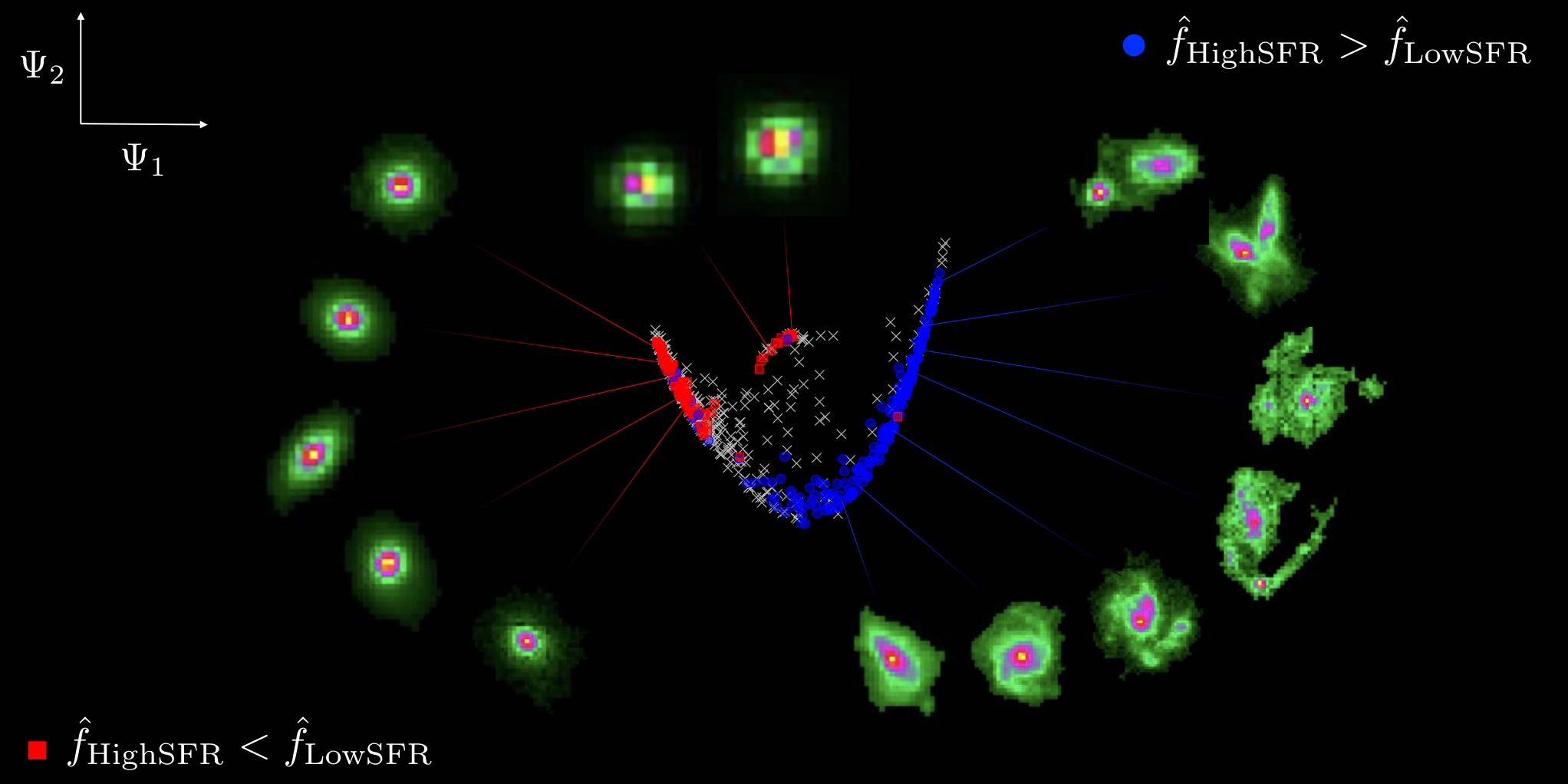
We illustrate the efficacy of the proposed global and local testing framework on the morphology statistics of two galaxy populations with high and low star-formation rate (SFR), respectively. The challenge here is not only that the problem involves multivariate data, but also that some of the morphological statistics are mixed discrete and continuous type with heavy outliers. We efficiently handle this issue by building on the success of random forests regression. The visualized local two-sample result is shown in Figure 1 and the details of the analysis can be found in Section 6.

In recent years, several attempts have been made to connect binary classification with two-sample testing. The main idea of this approach is to check whether the accuracy of a binary classifier is better than chance level and reject the null if the difference is significant. Such an approach, referred to as an accuracy or classification test, was conceptualized by Friedman, 2003 and has since been investigated by several authors (Ojala and Garriga, 2010; Olivetti et al., 2015; Kim et al., 2016; Rosenblatt et al., 2016; Gagnon-Bartsch and Shem-Tov, 2016; Lopez-Paz and Oquab, 2016; Hediger et al., 2019). In the same manner as our regression framework, a key strength of the accuracy test is that it offers a flexible way for the two-sample problem as it can utilize any existing classification procedure in the literature. However, the classification accuracy framework is not easily converted to a local two-sample test. In addition, many classifiers are estimated by dichotomizing regression estimators and the discrete nature of such classifiers may result in a less powerful test (see Section 5.2 and other simulation results).

For the global two-sample test, our framework can be viewed as an instance of goodness-of-fit testing for regression models (e.g. González-Manteiga and Crujeiras, 2013, for a review). There is a substantive literature on this topic including Hardle and Mammen, 1993, Weihrather, 1993, González-Manteiga and Cao, 1993, Zheng, 1996, Zhang and Dette, 2004, Hart, 2013 and among others. This line of work typically concentrates on comparing differences between parametric (e.g. linear regression) and nonparametric (e.g. kernel regression) fits from an asymptotic point of view. For example, Hardle and Mammen, 1993 consider the squared deviation between a parametric regression estimator and a kernel estimator. They show that their test statistic converges to a normal distribution under the null hypothesis and justify the use of the wild bootstrap procedure. However, this type of asymptotic approach is challenging to analyze beyond kernel-type estimators and often requires strong technical assumptions. In contrast, our framework is designed to compare any type of regression estimators with a specific constant fit by building upon the permutation principle. Hence the resulting test is valid in any finite sample sizes. Moreover we present a unified framework of studying the power of the regression test by taking advantage of existing results on the estimation error.

For the local two-sample test, our approach has similarities to independent work by Cazáis and Lhéritier, 2015 who estimate the Kullback-Leibler divergence between $\mathbb{P}(Y=1|X=x)$ and $\mathbb{P}(Y=1)$. Our procedure, however, identifies locally significant areas with statistical confidence whereas Cazáis and Lhéritier, 2015 graphically decide a threshold for the significance.

We outline the paper as follows: In Section 2, we introduce the proposed metrics, test statistics and algorithms for the global and local regression tests. In Section 3, we study theoretical properties of the global regression test. We begin by considering a simple scenario where two populations only differ in their means in Section 3.1. In this scenario, we show that the regression test based on Fisher’s linear discriminant analysis (LDA) achieves the same local optimality as the Hotelling’s $T^{2}$ test. Moving on to general regression settings in Section 3.2, we establish a connection between the testing error of the global regression test and the mean integrated square error (MISE) of the regression estimator. In Section 4, we turn to the local two-sample problem and investigate general properties of the local regression tests. In Section 4.1, we describe the testing error of the local regression test in terms of the mean square error (MSE) of the regression estimator. We further establish an optimality of the local regression tests over the Lipschitz class from a minimax point of view in Section 4.2. When data have intrinsic dimension, we show that the performance of the local regression tests based on kNN or kernel regression only depends on intrinsic dimension in Section 4.3. Section 4.4 studies the limiting distribution of the local permutation statistic to avoid a high computational cost from permutations for large sample size. In Section 5, simulation studies are provided to illustrate finite sample performance of the global and local regression tests. In Section 6, we apply the proposed approach to a problem in astronomy and demonstrate its efficacy. All the proofs are deferred to Appendix A.

A common metric for comparing two distributions is the difference between two density functions $f_{0}(x)$ and $f_{1}(x)$; this metric has been used for global and local two-sample testing by Anderson et al., 1994 and Duong, 2013. Another natural metric, suggested for global two-sample testing by Keziou and Leoni-Aubin, 2005, Fokianos, 2008 and Sugiyama et al., 2011, is the density ratio $f_{1}(x)/f_{0}(x)$. Although both the density difference and density ratio metrics are intuitive, there are several weaknesses associated with each of them. For example, the estimation of a density difference is largely limited to kernel density estimators, which are sensitive to the curse of dimensionality. The density ratio, on the other hand, could potentially be estimated using various regression methods thanks to the following reformulation:

$\displaystyle\frac{f_{1}(x)}{f_{0}(x)}=\frac{\pi_{0}}{\pi_{1}}\frac{m(x)}{1-m(x)},$

(Qin and Zhang, 1997, see, e.g.,). The main weakness of the ratio approach, however, is that the ratio is highly sensitive to the tail behavior of distributions, and it is not even well defined when $m(x)=1$. To overcome these limitations, we propose an alternative approach which instead compares the regression function with the class probability. More specifically, we consider

$\displaystyle\mathcal{T}_{global}=\int_{S}\{m(x)-\pi_{1}\}^{2}dP_{X}(x),\quad\mathcal{T}_{local}(x)=\{m(x)-\pi_{1}\}^{2}$

(2)

as global and local measures of the discrepancy between two distributions where we assume that $\pi_{1}$ is a fixed constant within $0<\pi_{1}<1$ throughout this paper. By construction, both $\mathcal{T}_{global}$ and $\mathcal{T}_{local}(x)$ are bounded between zero and one. More importantly, we can take advantage of numerous existing regression methods (see, e.g., Friedman et al., 2009, for popular methods and descriptions) when estimating $m(x)$. Hence, our approach maintains the flexibility of the density ratio approach while avoiding the problem of ill-defined quantities.

Suppose we observe $n$ pairs of samples $\{(X_{i},Y_{i})\}_{i=1}^{n}$, where $X_{i}\in\mathbb{R}^{D}$ and $Y_{i}\in\{0,1\}$. Let $\widehat{m}(x)$ be an estimate of $m(x)$ based on the samples, and $\widehat{\pi}_{1}=\frac{1}{n}\sum_{i=1}^{n}I(Y_{i}=1)$. Then by plugging these statistics into (2), we define our global and local test statistics as

$\displaystyle\widehat{\mathcal{T}}_{global}=\frac{1}{n}\sum_{i=1}^{n}\{\widehat{m}(X_{i})-\widehat{\pi}_{1}\}^{2},\quad\widehat{\mathcal{T}}_{local}(x)=\{\widehat{m}(x)-\widehat{\pi}_{1}\}^{2}.$

(3)

The null distributions of the proposed test statistics are typically unknown, and they depend on the choice of regression method as well as the distribution of the data. Hence, to keep our framework as general as possible, we use a permutation procedure to set a critical value that yields a valid level $\alpha$ test for any given regression estimator under any sampling scheme given in Section 2.3. The proposed permutation framework for global and local two-sample testing are summarized in Algorithm 1 and Algorithm 2, respectively.

In the two-sample problem, there are two common sampling schemes for obtaining the paired data set $\{(X_{i},Y_{i})\}_{i=1}^{n}$, namely i) i.i.d. sampling and ii) separate sampling defined as follows:

• •

  i.i.d. sampling. Under i.i.d. sampling, we observe $n$ pairs of i.i.d. samples $\{(X_{i},Y_{i})\}_{i=1}^{n}$ from the joint distribution $\pi_{1}[P_{1}\times\delta_{1}]+\pi_{0}[P_{0}\times\delta_{0}]$. Here we note that $n$ is fixed in advance. Then $n_{1}=\sum_{i=1}^{n}I(Y_{i}=1)$ and $n_{0}=n-n_{1}$ are $\text{Binomial}(n,\pi_{1})$ and $\text{Binomial}(n,\pi_{0})$, respectively. This setting is common in applications of supervised learning where the goal is to build a model that can successfully predict the class label $Y$ given the feature vector $X$ (Friedman et al., 2009, e.g.). Our goal, on the other hand, is to test whether the two distributions $P_{0}$ and $P_{1}$ are the same or not by leveraging existing methods in the regression literature.
  

• •

  Separate sampling. In the case of separate sampling, $n_{0}$ and $n_{1}$ are predetermined and they are not random. We then observe $n_{0}$ and $n_{1}$ independent sample points from $P_{0}$ and $P_{1}$ separately, which provides the data set $\{(X_{i},Y_{i})\}_{i=1}^{n}$ where $Y_{i}=1$ if $X_{i}$ was drawn from $P_{1}$ and $Y_{i}=0$ otherwise.

We can link the separate sampling to the i.i.d. sampling scheme by randomly ordering the $(X_{i},Y_{i})$ pairs, so that the data points are exchangeable and for each $i\in\{1,\ldots,n\}$, the conditional distribution of $Y_{i}$ given $X_{i}=x$ is $m(x)=\pi_{1}f_{1}(x)/\{\pi_{1}f_{1}(x)+\pi_{0}f_{0}(x)\}$ where the class probability is given by $\pi_{1}=n_{1}/n$. Therefore, although the joint distributions of $\{(X_{i},Y_{i})\}_{i=1}^{n}$ are different under i.i.d. and separate sampling schemes, they share the same regression function.

In this section, we consider a simple scenario of two sample normal mean to highlight the difference between our approach and the classification accuracy approach. In particular, we prove that the regression test based on Fisher’s LDA achieves the same local power as Hotelling’s $T^{2}$ test. This result has significance given that i) Hotelling’s test is optimal under the considered scenario and ii) the classification accuracy test based on Fisher’s LDA is usually underpowered (Kim et al., 2016; Rosenblatt et al., 2016). To facilitate comparison with the previous results, which are established under separate sampling, we also consider the case where $n_{0}$ and $n_{1}$ are predetermined throughout this subsection.

Suppose we observe $\{X_{i,0}\}_{i=1}^{n_{0}}\overset{i.i.d.}{\sim}N(\mu_{0},\Sigma)$ and independently $\{X_{i,1}\}_{i=1}^{n_{1}}\overset{i.i.d.}{\sim}N(\mu_{1},\Sigma)$. We denote the pooled samples by $\{X_{i}\}_{i=1}^{n}=\{X_{i,0}\}_{i=1}^{n_{0}}\cup\{X_{i,1}\}_{i=1}^{n_{1}}$ where $n=n_{0}+n_{1}$. The two-sample problem then becomes the problem of testing for mean differences as

$\displaystyle H_{0}:\mu_{0}=\mu_{1}\quad\text{versus}\quad H_{1}:\mu_{0}\neq\mu_{1}.$

(4)

For this particular problem, Fisher’s LDA is a natural choice for regression, assuming normality and equal class covariances. Let $\widehat{\mu}_{i}$ be the sample mean vector for each group, $\mathcal{S}$ be the covariance matrix of the combined samples, i.e. $\mathcal{S}=n^{-1}\sum_{i=1}^{n}(X_{i}-\widehat{\mu})(X_{i}-\widehat{\mu})^{\top}$ where $\widehat{\mu}=n^{-1}\sum_{i=1}^{n}X_{i}$. Then, by putting $\pi_{1}=n_{1}/n$, the regression estimator based on Fisher’s LDA is given by

$\displaystyle\widehat{m}_{\text{LDA}}(x)=\frac{\pi_{1}\exp\big\{-\frac{1}{2}(x-\widehat{\mu}_{1})^{\top}\mathcal{S}^{-1}(x-\widehat{\mu}_{1})\big\}}{\pi_{0}\exp\big\{-\frac{1}{2}(x-\widehat{\mu}_{0})^{\top}\mathcal{S}^{-1}(x-\widehat{\mu}_{0})\big\}+\pi_{1}\exp\big\{-\frac{1}{2}(x-\widehat{\mu}_{1})^{\top}\mathcal{S}^{-1}(x-\widehat{\mu}_{1})\big\}}.$

(5)

One of the most popular test statistics for testing (4) is Hotelling’s $T^{2}$ statistic, which yields optimal power for the normal means problem (Anderson, 2003, see, e.g.). For the two-sample problem, Hotelling’s $T^{2}$ statistic is defined by

$\displaystyle T^{2}_{\text{Hotelling}}=\frac{n_{0}n_{1}}{n_{0}+n_{1}}(\widehat{\mu}_{0}-\widehat{\mu}_{1})^{\top}\mathcal{S}_{p}^{-1}(\widehat{\mu}_{0}-\widehat{\mu}_{1}),$

where $\mathcal{S}_{p}$ is the pooled covariance matrix, that is

$\displaystyle\mathcal{S}_{p}=\frac{1}{n_{0}+n_{1}-2}\left(\sum_{i=1}^{n_{0}}(X_{i,0}-\widehat{\mu}_{0})(X_{i,0}-\widehat{\mu}_{0})^{\top}+\sum_{i=1}^{n_{1}}(X_{i,1}-\widehat{\mu}_{1})(X_{i,1}-\widehat{\mu}_{1})^{\top}\right).$

On the other hand, the regression test statistic based on Fisher’s LDA is given by

$\displaystyle\widehat{\mathcal{T}}_{\text{LDA}}=\frac{1}{n}\sum_{i=1}^{n}\Big(\widehat{m}_{\text{LDA}}(X_{i})-\pi_{1}\Big)^{2}.$

The next theorem provides a connection between the seemingly unrelated $\widehat{\mathcal{T}}_{\text{LDA}}$ and $T^{2}_{\text{Hotelling}}$ statistics. Specifically, it shows that $n{\pi_{0}^{-1}\pi_{1}^{-1}}\widehat{\mathcal{T}}_{\text{LDA}}$ is asymptotically identical to Hotelling’s $T^{2}$ statistic under the null. It is also worth pointing out that the theorem still holds without the normality assumption.

Let us now turn to the alternative hypothesis. To begin with, we consider a family of probability functions that satisfy the following smoothness condition.

Such q.m.d. families include fairly large parametric models such as exponential families in natural form. For our purpose, we focus on location q.m.d. families, denoted by $\{\mathbb{P}_{\mu},\mu\in\Omega\}$. Specifically, $\mathbb{P}_{\mu}$ is a member of $\{\mathbb{P}_{\mu},\mu\in\Omega\}$ if its density satisfies $f_{\mu}(x)=f(x-\mu)$ for which $f(x)$ has zero mean and covariance matrix $\Sigma$. Next, for given $\mathbb{P}_{\mu_{0}}$ and $\mathbb{P}_{\mu_{1}}$ from $\{\mathbb{P}_{\mu},\mu\in\Omega\}$, let us consider the local alternative

$\displaystyle H_{1,n}:\mu_{1}-\mu_{0}=h/\sqrt{n},$

(8)

where $h=(h_{1},\ldots,h_{D})^{\top}$. Then, under $H_{1,n}$, $\widehat{\mathcal{T}}_{\text{LDA}}$ has asymptotic behavior as follows.

The results from Theorem 3.1 and Theorem 3.2 imply that our regression test based on $\widehat{\mathcal{T}}_{\text{LDA}}$ has the same asymptotic local power as Hotelling’s $T^{2}$ test. As a result, the regression test based on $\widehat{\mathcal{T}}_{\text{LDA}}$ is asymptotically optimal against the local alternatives as Hotelling’s $T^{2}$ test.

To illustrate the main point of this section, we compare the performance of $\widehat{\mathcal{T}}_{\text{LDA}}$ with Hotelling’s $T^{2}$ test through Monte Carlo simulations. We randomly generate $n_{0}=n_{1}=100$ samples from $N((0,\ldots,0)^{\top},I_{D})$ and $N((\mu,\ldots,\mu)^{\top},I_{D})$, respectively and set $\mu^{2}=0.05$ for $D=5$ and $\mu^{2}=0.01$ for $D=20$. We also consider two versions of the accuracy-based tests via Fisher’s LDA: the in-sample (re-substitution) accuracy and the two-fold cross-validated accuracy. To calculate the cross-validated accuracy, we use the balanced sample splitting scheme in which the first part of data is used to train the LDA, and the second part is used to estimate the accuracy of the classifier (see, Definition 1 and 2 of Rosenblatt et al., 2016, for more details). To make a fair comparison, the critical values of the given tests were all decided by the permutation procedure. As shown in Figure 2, the regression test based on $\widehat{\mathcal{T}}_{\text{LDA}}$ has comparable power to Hotelling’s $T^{2}$ test that coincides with our theory. On the other hand, the accuracy tests have less power than Hotelling’s $T^{2}$ test.

We now turn to more general regression settings and investigate general properties of the global regression test in both separate and i.i.d. sampling cases. Let $\mathcal{M}$ be a certain class of regression $m(x):S\subseteq\mathbb{R}^{D}\mapsto[0,1]$ containing constant functions. Suppose that we have a regression estimator $\widehat{m}(x)$ that has the mean integrated square error as

$\displaystyle\sup_{m\in\mathcal{M}}\mathbb{E}\int_{S}\left(\widehat{m}(x)-m(x)\right)^{2}dP_{X}(x)\leq C_{0}\delta_{n},$

(9)

where $C_{0}$ is a positive constant and $\delta_{n}=o(1)$. In the case of i.i.d. sampling, we further assume $\delta_{n}\geq n^{-1}$, which is typical for nonparametric regression estimators. Our main interest here is in employing the above MISE to characterize the testing error of the global regression test. Note that the plug-in global statistic in (3) is typically a biased estimator of the MISE and the bias differs from case to case. To simplify our analysis, we consider sample splitting where the half of data is used to estimate the regression function and the other is used to evaluate the empirical squared error. In detail, given samples $(X_{1},Y_{1}),\ldots,(X_{2n},Y_{2n})$, the regression test statistic based on (random) sample splitting is defined by

$\displaystyle\widehat{\mathcal{T}}_{global}^{\prime}=\frac{1}{n}\sum_{i=n+1}^{2n}\left(\widehat{m}(X_{i})-\widehat{\pi}_{1}\right)^{2},$

(10)

where $\widehat{m}(\cdot)$ and $\widehat{\pi}_{1}$ are calculated based on the first half of the data $\{(X_{1},Y_{1}),\ldots,(X_{n},Y_{n})\}$. In the case of separate sampling, we assume a random ordering in the entire data set and similarly split it into two parts but with the additional restriction that class probabilities are the same in both parts. Based on $\widehat{\mathcal{T}}_{global}^{\prime}$, we argue that for sufficiently large $C_{1}>0$ and $n$, the testing error of the global regression test can be arbitrarily small against the class of global alternatives given by

$\displaystyle\mathcal{M}(C_{1}\delta_{n})=\Big\{m\in\mathcal{M}:\int_{S}\left(m(x)-\pi_{1}\right)^{2}dP_{X}(x)\geq C_{1}\delta_{n}\Big\}.$

Note that since $\pi_{1}$ is assumed to be fixed, the regression function $m(x)$ is completely determined by $f_{0}$ and $f_{1}$. Thus in the following theorem and hereafter, we use the notation $f_{0},f_{1}\in\mathcal{M}$ to represent $m(x)=\pi_{1}f_{1}(x)/\{\pi_{0}f_{0}(x)+\pi_{1}f_{1}(x)\}\in\mathcal{M}$. Similarly, we write $f_{0},f_{1}\in\mathcal{M}_{0}$ to signify that $\pi_{1}f_{1}(x)/\{\pi_{0}f_{0}(x)+\pi_{1}f_{1}(x)\}=\pi_{1}$ for all $x\in S$. With this notation in hand, we state the main theorem of this subsection.

Theorem 3.3 uses the assumption that the permutation critical value of the regression test is uniformly bounded by $\delta_{n}$ (up to some constant factor) with high probability. We end this subsection with a class of regression estimators, which satisfy this assumption. Let us consider a class of regression estimators with the following representation:

$\displaystyle\widehat{m}(x)=\sum_{i=1}^{n}w_{i}(x)Y_{i},$

where $w_{i}(x)\geq 0$ and $\sum_{i=1}^{n}w_{i}(x)=1$ for all $x$. In addition, we assume that $w_{i}(x)$ is a function of $\{X_{1},\ldots,X_{n}\}$ but not $\{Y_{1},\ldots,Y_{n}\}$. This class of estimators, often called linear smoothers, contains many popular regression methods such as k-nearest neighbor (kNN) regression, kernel regression and local polynomial regression. Focusing on linear smoothers, we provide the following corollary.

In the case of i.i.d. sampling, the convergence rate $\delta_{n}$ of commonly used regression estimators have been well-established and these results can be directly used to study the testing error of the global regression test. We list several known results here. More examples can be found in Györfi et al., 2002, Tsybakov, 2009 and Devroye et al., 2013.

• •

  kNN regression.  When $\mathcal{M}$ is a class of Lipschitz continuous functions, the convergence rate of kNN estimators satisfies $\delta_{n}=n^{-2/(2+D)}$ (Györfi et al., 2002). This can be generalized to a Hölder space with smooth parameter $\beta$ in which the rate becomes $\delta_{n}=n^{-2\beta/(2\beta+D)}$ (Györfi et al., 2002; Ayano, 2012) for $0<\beta\leq 1.5$. Furthermore, Kpotufe, 2011 shows that kNN estimators are adaptive to the intrinsic dimension $d\ll D$ under appropriate conditions. In this case, the convergence rate becomes much faster as $\delta_{n}=n^{-2/(2+d)}\ll n^{-2/(2+D)}$.
  

• •

  Kernel regression.  Kernel regression estimators also achieve the converge rate as $\delta_{n}=n^{-2/(2+D)}$ for Lipschitz continuous functions and more generally as $\delta_{n}=n^{-2\beta/(2\beta+D)}$ for a Hölder space with smooth parameter $0<\beta\leq 1.5$ (Györfi et al., 2002). The adaptivity of kernel regression to the intrinsic dimension has been proved by Kpotufe and Garg, 2013. Following their results, the convergence rate becomes $\delta_{n}=n^{-2/(2+d)}\ll n^{-2/(2+D)}$ when there exists a low-dimensional structure in the data.
  

• •

  Local polynomial regression.  Let $\mathcal{M}$ be a Sobolev space with smoothness $\alpha$. Then local polynomial regression estimators has the convergence rate as $\delta_{n}=n^{-\alpha/(\alpha+d)}$ where $d$ is manifold dimension smaller than the original dimension $D$ (Bickel and Li, 2007).
  

• •

  Random forests regression.  For Lipschitz continuous functions, Biau, 2012 shows that the random forest estimator converges at rate $\delta_{n}=n^{-\frac{0.75}{s\log 2+0.75}}$ where $s$ is the number of the relevant features. Hence, the convergence rate of the random forests becomes faster than $n^{-2/(2+D)}$ when $s\leq D/2$ under certain conditions. Wager and Walther, 2015 use the guess-and-check forest algorithm to show that the convergence rate of the random forest is $\delta_{n}=n^{-\log(\xi)/\log(2\xi)}$ where $\xi=1/(1-3/4s)$.

To the best of our knowledge, there has been no detailed investigation of the regression estimation error under separate sampling. In this case, we cannot directly take advantage of existing results on regression. However, as the sample size becomes larger, the difference between i.i.d. sampling and separate sampling becomes minor. Hence we expect that a reasonable regression estimator behaves similarly under both sampling schemes in large sample sizes, while a detailed analysis is necessary in future work. It is also worth noting that for certain regression methods, consistency results are not significantly affected by sampling scheme. For example, the consistency theory for $L_{1}$ penalized regression relies mainly on the assumption about a design matrix, which can be fulfilled under both sampling schemes (Van de Geer, 2008; Bühlmann and Van De Geer, 2011). In such a case, the same convergence rate can be established under both sampling schemes.

We start by establishing similar results in Section 3.2 for local regression tests. Given a local point $x\in S$ of interest, suppose that a regression estimator has the mean square error such that

$\displaystyle\sup_{m\in\mathcal{M}}\mathbb{E}\left[\left(\widehat{m}(x)-m(x)\right)^{2}\right]\leq C_{0,x}\delta_{n,x},$

(11)

where $C_{0,x}$ is a positive constant and $\delta_{n,x}=o(1)$. In addition, we assume $\delta_{n,x}\geq n^{-1}$ for i.i.d. sampling. Then the next theorem shows that for sufficiently large $C_{1,x}$ and $n$, the local testing error based on the given regression estimator can be arbitrarily small against the class of local alternatives given by

$\displaystyle\mathcal{M}(C_{1,x}\delta_{n,x})=\Big\{m\in\mathcal{M}:\left(m(x)-\pi_{1}\right)^{2}\geq C_{1,x}\delta_{n,x}\Big\}.$

In order to keep things as simple and concrete as possible, we next focus on the Lipschitz class and analyze the optimality of the local regression tests from a minimax point of view. In the rest of this section (Section 4.2–4.4), we concentrate on i.i.d. sampling scheme to take full advantage of known regression results. However, as we discussed in Section 3.3, similar results are expected to hold under separate sampling as well.

For a fixed constant $L>0$, let us denote the Lipschitz function class by

$\displaystyle\mathcal{M}_{Lip}=\Big\{m:|m(x)-m(y)|\leq L||x-y||_{2}~\text{for all $x,y\in S$}\Big\}.$

We also denote the collection of $\alpha$ level tests by $\Phi_{n,\alpha}=\{\phi:\sup_{f_{0},f_{1}\in\mathcal{M}_{0}}\mathbb{P}_{f_{0},f_{1}}(\phi=1)\leq\alpha\}$ and denote the class of Lipschitz local alternatives by

$\displaystyle\mathcal{M}_{Lip}(\delta_{n,x})=\Big\{m\in\mathcal{M}_{Lip}:\left(m(x)-\pi_{1}\right)^{2}\geq\delta_{n,x}\Big\}.$

(12)

With this notation and fixed $\alpha\in(0,1)$ and $\beta\in(0,1-\alpha)$, the minimum separation is defined by

$\displaystyle\delta_{n,x}^{\star}=\inf\Big\{\delta_{n,x}:\inf_{\phi\in\Phi_{n,\alpha}}\sup_{f_{0},f_{1}\in\mathcal{M}_{Lip}(\delta_{n,x})}\mathbb{P}_{f_{0},f_{1}}(\phi=0)\leq\beta\Big\},$

(13)

which is the smallest distance between $m(x)$ and $\pi_{1}$ such that the power becomes nontrivial. Then a test is called minimax rate optimal if it has power uniformly over $\mathcal{M}_{Lip}(\delta_{n,x})$ such that $\delta_{n,x}\asymp\delta_{n,x}^{\star}$.

In this section, we will investigate minimax rate optimality of local regression tests over the Lipschitz class under i.i.d. sampling. First we formally state an upper bound for the local estimation error based on kNN and kernel regression in Example 4.1 and Example 4.2, respectively. We then use these results to obtain the upper bound for the minimum separation in Corollary 4.1.

A similar result can be established for kernel regression estimators as follows.

References

- Anderson, (1972) Anderson, J. A. (1972). Separate sample logistic discrimination. Biometrika, 59(1):19–35.
- Anderson et al., (1994) Anderson, N. H., Hall, P., and Titterington, D. M. (1994). Two-sample test statistics for measuring discrepancies between two multivariate probability density functions using kernel-based density estimates. Journal of Multivariate Analysis, 50(1):41–54.
- Anderson, (2003) Anderson, T. W. (2003). An Introduction to Multivariate Statistical Analysis, volume 3. New York: Wiley-Interscience.
- Ayano, (2012) Ayano, T. (2012). Rates of convergence for the k-nearest neighbor estimators with smoother regression functions. Journal of Statistical Planning and Inference, 142(9):2530–2536.
- Baraud, (2002) Baraud, Y. (2002). Non-asymptotic minimax rates of testing in signal detection. Bernoulli, 8(5):577–606.
- Baringhaus and Franz, (2004) Baringhaus, L. and Franz, C. (2004). On a new multivariate two-sample test. Journal of Multivariate Analysis, 88(1):190–206.
- Biau, (2012) Biau, G. (2012). Analysis of a random forests model. Journal of Machine Learning Research, 13(Apr):1063–1095.
- Biau and Devroye, (2015) Biau, G. and Devroye, L. (2015). Lectures on the nearest neighbor method. Springer.
- Bickel and Li, (2007) Bickel, P. J. and Li, B. (2007). Local polynomial regression on unknown manifolds. Lecture Notes-Monograph Series, pages 177–186.
- Bolthausen, (1984) Bolthausen, E. (1984). An estimate of the remainder in a combinatorial central limit theorem. Zeitschrift für Wahrscheinlichkeitstheorie und verwandte Gebiete, 66(3):379–386.
- Breiman, (2001) Breiman, L. (2001). Random forests. Machine learning, 45(1):5–32.
- Bühlmann and Van De Geer, (2011) Bühlmann, P. and Van De Geer, S. (2011). Statistics for high-dimensional data: methods, theory and applications. Springer Science & Business Media.
- Bunea and Barbu, (2009) Bunea, F. and Barbu, A. (2009). Dimension reduction and variable selection in case control studies via regularized likelihood optimization. Electronic Journal of Statistics, 3:1257–1287.
- Cazáis and Lhéritier, (2015) Cazáis, F. and Lhéritier, A. (2015). Beyond two-sample-tests: Localizing data discrepancies in high-dimensional spaces. In Data Science and Advanced Analytics (DSAA), 2015. 36678 2015. IEEE International Conference on, pages 1–10. IEEE.
- Chen and Ishwaran, (2012) Chen, X. and Ishwaran, H. (2012). Random forests for genomic data analysis. Genomics, 99(6):323–329.
- Coifman and Lafon, (2006) Coifman, R. R. and Lafon, S. (2006). Diffusion maps. Applied and computational harmonic analysis, 21(1):5–30.
- Coifman et al., (2005) Coifman, R. R., Lafon, S., Lee, A. B., Maggioni, M., Nadler, B., Warner, F., and Zucker, S. W. (2005). Geometric diffusions as a tool for harmonic analysis and structure definition of data: Diffusion maps. Proceedings of the National Academy of Sciences of the United States of America, 102(21):7426–7431.
- Conselice, (2003) Conselice, C. J. (2003). The relationship between stellar light distributions of galaxies and their formation histories. The Astrophysical Journal Supplement Series, 147(1):1.
- Conselice, (2014) Conselice, C. J. (2014). The evolution of galaxy structure over cosmic time. Annual Review of Astronomy and Astrophysics, 52:291–337.
- Cutler et al., (2007) Cutler, D. R., Edwards, T. C., Beard, K. H., Cutler, A., Hess, K. T., Gibson, J., and Lawler, J. J. (2007). Random forests for classification in ecology. Ecology, 88(11):2783–2792.
- Devroye et al., (2013) Devroye, L., Györfi, L., and Lugosi, G. (2013). A probabilistic theory of pattern recognition, volume 31. Springer Science & Business Media.
- Díaz-Uriarte and De Andres, (2006) Díaz-Uriarte, R. and De Andres, S. A. (2006). Gene selection and classification of microarray data using random forest. BMC bioinformatics, 7(1):3.
- Duong, (2013) Duong, T. (2013). Local significant differences from nonparametric two-sample tests. Journal of Nonparametric Statistics, 25(3):635–645.
- Fokianos, (2008) Fokianos, K. (2008). Comparing two samples by penalized logistic regression. Electronic Journal of Statistics, 2:564–580.
- Freeman et al., (2013) Freeman, P., Izbicki, R., Lee, A., Newman, J., Conselice, C., Koekemoer, A., Lotz, J., and Mozena, M. (2013). New image statistics for detecting disturbed galaxy morphologies at high redshift. Monthly Notices of the Royal Astronomical Society, 434(1):282–295.
- Friedman et al., (2009) Friedman, J., Hastie, T., and Tibshirani, R. (2009). The Elements of Statistical Learning. Springer, New York.
- Friedman, (2003) Friedman, J. H. (2003). On multivariate goodness of fit and two sample testing. eConf, 30908(SLAC-PUB-10325):311–313.
- Gagnon-Bartsch and Shem-Tov, (2016) Gagnon-Bartsch, J. and Shem-Tov, Y. (2016). The classification permutation test: A nonparametric test for equality of multivariate distributions. arXiv preprint arXiv:1611.06408.
- González-Manteiga and Cao, (1993) González-Manteiga, W. and Cao, R. (1993). Testing the hypothesis of a general linear model using nonparametric regression estimation. Test, 2(1-2):161–188.
- González-Manteiga and Crujeiras, (2013) González-Manteiga, W. and Crujeiras, R. M. (2013). An updated review of goodness-of-fit tests for regression models. Test, 22(3):361–411.
- Gretton et al., (2012) Gretton, A., Borgwardt, K. M., Rasch, M. J., Schölkopf, B., and Smola, A. (2012). A kernel two-sample test. Journal of Machine Learning Research, 13(Mar):723–773.
- Györfi et al., (2002) Györfi, L., Kohler, M., Krzyzak, A., and Walk, H. (2002). A distribution-free theory of nonparametric regression. Springer Science & Business Media.
- Hamza and Larocque, (2005) Hamza, M. and Larocque, D. (2005). An empirical comparison of ensemble methods based on classification trees. Journal of Statistical Computation and Simulation, 75(8):629–643.
- Hardle and Mammen, (1993) Hardle, W. and Mammen, E. (1993). Comparing nonparametric versus parametric regression fits. The Annals of Statistics, 21(4):1926–1947.
- Hart, (2013) Hart, J. (2013). Nonparametric smoothing and lack-of-fit tests. Springer Science & Business Media.
- Hediger et al., (2019) Hediger, S., Michel, L., and Näf, J. (2019). On the use of random forest for two-sample testing. arXiv preprint arXiv:1903.06287.
- Hochberg, (1988) Hochberg, Y. (1988). A sharper bonferroni procedure for multiple tests of significance. Biometrika, 75(4):800–802.
- Hu and Bai, (2016) Hu, J. and Bai, Z. (2016). A review of 20 years of naive tests of significance for high-dimensional mean vectors and covariance matrices. Science China Mathematics, 59(12):2281–2300.
- Ingster, (1987) Ingster, Y. I. (1987). Minimax testing of nonparametric hypotheses on a distribution density in the l_p metrics. Theory of Probability & Its Applications, 31(2):333–337.
- Keziou and Leoni-Aubin, (2005) Keziou, A. and Leoni-Aubin, S. (2005). Test of homogeneity in semiparametric two-sample density ratio models. Comptes Rendus Mathématique, 340(12):905–910.
- Kim et al., (2016) Kim, I., Ramdas, A., Singh, A., and Wasserman, L. (2016). Classification Accuracy as a Proxy for Two Sample Testing. arXiv preprint arXiv:1602.02210.
- Kpotufe, (2011) Kpotufe, S. (2011). k-NN regression adapts to local intrinsic dimension. In Advances in Neural Information Processing Systems, pages 729–737.
- Kpotufe and Garg, (2013) Kpotufe, S. and Garg, V. (2013). Adaptivity to local smoothness and dimension in kernel regression. In Advances in neural information processing systems, pages 3075–3083.
- Lehmann and Romano, (2006) Lehmann, E. L. and Romano, J. P. (2006). Testing statistical hypotheses. Springer Science & Business Media.
- Lopez-Paz and Oquab, (2016) Lopez-Paz, D. and Oquab, M. (2016). Revisiting classifier two-sample tests. arXiv preprint arXiv:1610.06545.
- Lotz et al., (2004) Lotz, J. M., Primack, J., and Madau, P. (2004). A new nonparametric approach to galaxy morphological classification. The Astronomical Journal, 128(1):163.
- Mondal et al., (2015) Mondal, P. K., Biswas, M., and Ghosh, A. K. (2015). On high dimensional two-sample tests based on nearest neighbors. Journal of Multivariate Analysis, 141:168–178.
- Ojala and Garriga, (2010) Ojala, M. and Garriga, G. C. (2010). Permutation tests for studying classifier performance. Journal of Machine Learning Research, 11(Jun):1833–1863.
- Olivetti et al., (2015) Olivetti, E., Greiner, S., and Avesani, P. (2015). Statistical independence for the evaluation of classifier-based diagnosis. Brain Informatics, 2(1):13–19.
- Prentice and Pyke, (1979) Prentice, R. L. and Pyke, R. (1979). Logistic disease incidence models and case-control studies. Biometrika, 66(3):403–411.
- Qin and Zhang, (1997) Qin, J. and Zhang, B. (1997). A goodness-of-fit test for logistic regression models based on case-control data. Biometrika, pages 609–618.
- Ramdas et al., (2015) Ramdas, A., Reddi, S. J., Poczos, B., Singh, A., and Wasserman, L. (2015). Adaptivity and computation-statistics tradeoffs for kernel and distance based high dimensional two sample testing. arXiv preprint arXiv:1508.00655.
- Rosenblatt et al., (2016) Rosenblatt, J., Gilron, R., and Mukamel, R. (2016). Better-than-chance classification for signal detection. arXiv preprint arXiv:1608.08873.
- Scott and Wild, (2001) Scott, A. J. and Wild, C. (2001). Maximum likelihood for generalised case-control studies. Journal of Statistical Planning and Inference, 96(1):3–27.
- Snyder et al., (2015) Snyder, G. F., Torrey, P., Lotz, J. M., Genel, S., McBride, C. K., Vogelsberger, M., Pillepich, A., Nelson, D., Sales, L. V., and Sijacki, D. (2015). Galaxy morphology and star formation in the illustris simulation at z= 0. Monthly Notices of the Royal Astronomical Society, 454(2):1886–1908.
- Sugiyama et al., (2011) Sugiyama, M., Suzuki, T., Itoh, Y., Kanamori, T., and Kimura, M. (2011). Least-squares two-sample test. Neural Networks, 24(7):735–751.
- Székely and Rizzo, (2004) Székely, G. J. and Rizzo, M. L. (2004). Testing for equal distributions in high dimension. InterStat, 5:1–6.
- Thas, (2010) Thas, O. (2010). Comparing distributions. Springer.
- Tsybakov, (2009) Tsybakov, A. B. (2009). Introduction to nonparametric estimation. Revised and extended from the 2004 French original. Translated by Vladimir Zaiats. Springer Series in Statistics. Springer, New York.
- Van de Geer, (2008) Van de Geer, S. A. (2008). High-dimensional generalized linear models and the lasso. The Annals of Statistics, 36(2):614–645.
- Wager and Walther, (2015) Wager, S. and Walther, G. (2015). Adaptive concentration of regression trees, with application to random forests. arXiv preprint arXiv:1503.06388.
- Wang and Carroll, (1993) Wang, C. and Carroll, R. (1993). On robust estimation in logistic case-control studies. Biometrika, 80(1):237–241.
- Wang and Carroll, (1999) Wang, S. and Carroll, R. J. (1999). High-order accurate methods for retrospective sampling problems. Biometrika, 86(4):881–897.
- Wasserman, (2006) Wasserman, L. (2006). All of nonparametric statistics. Springer Science & Business Media.
- Weihrather, (1993) Weihrather, G. (1993). Testing a linear regression model against nonparametric alternatives. Metrika, 40(1):367–379.
- Yang and Barron, (1999) Yang, Y. and Barron, A. (1999). Information-theoretic determination of minimax rates of convergence. Annals of Statistics, 27(5):1564–1599.
- Zelnik-Manor and Perona, (2005) Zelnik-Manor, L. and Perona, P. (2005). Self-tuning spectral clustering. In Advances in neural information processing systems, pages 1601–1608.
- Zhang and Dette, (2004) Zhang, C. and Dette, H. (2004). A power comparison between nonparametric regression tests. Statistics & probability letters, 66(3):289–301.
- Zheng, (1996) Zheng, J. X. (1996). A consistent test of functional form via nonparametric estimation techniques. Journal of Econometrics, 75(2):263–289.
Appendix A Proofs
A.1 Proof of Theorem 3.1
We start by simplifying as
and write
For some , Taylor expansion of at provides
where is a universal constant. This implies that
Now based on and Cauchy-Schwarz inequality, it can be seen that
As a result, can be approximated by