Bayesian Manifold-Constrained-Prior Model for an Experiment to Locate Xce

The Calaway et al. 2013 first established which Xce allele was carried by a few unclassified strains. Based upon the observations, a provisional, semi-statistical classification was assumed, and this motivated the choice to classify additional strains. First, strains SJL/J (SJL) and ALS/LtJ (ALS) were analyzed because their sequences split the known region between $\mbox{\emph{Xce}}^{a}$ and $\mbox{\emph{Xce}}^{b}$. Then strains LEWES/EiJ (LEWES) and WLA/Pas (WLA) followed. Additional crosses with WSB/EiJ (WSB), PWK/PhJ (PWK) were generated and measured, including some RNA-seq measurements. Available frozen $\text{F}_{2}$ samples of crosses including DDK/Pas (DDK), ZALENDE/Ei (ZALENDE), PERA/EiJ (PERA) (Nishioka 1995) were acquired. Some successful breedings with PANCEVO/EiJ (PANCEVO) (Kim et al. 2005) were conducted to see if this second species of mouse had a different Xce profile. Only a subset of possible crosses were performed, and not all reciprocal crosses were generated. Count of replicates per unique crosses varied from 4 to 50.

For convenience, summarizing details for the inbred parental strains are given in Table 1. A statistical analysis must respect that the experiment is adaptive and sequential in nature, that many crosses which might have aided in the statistical estimate will be missing, and that we should provide a statistical criterion not only to assert that a given cross SJL $\times\texttt{B6}$ has an average “$50.1\%\pm 2.1\%$”, but that we should also be able to express how certain we are that SJL is an $a$ allele carrier. By choosing closely related potential $\mbox{\emph{Xce}}^{a}$ and $\mbox{\emph{Xce}}^{b}$ allele carriers, predominantly from mus domesticus,  Calaway et al. 2013 proceeded with an investigation that, aided by this statistical analysis, refined the Xce location from the 1.9 Mega-base (Mb) Chadwick et al. 2006 candidate interval to a 176 kilo-base (kb) region approximately 500 kb from the gene Xist whose expression causes X-inactivation. Calaway et al. 2013 established that allele $\mbox{\emph{Xce}}^{a}$ is rare in the wild and that most individuals within a sub-species share the same Xce allele. They found that Xce-allele strengths can potentially increase or decrease during speciation, which suggests Xce is mutated through copy number variation.

A partial Table 2 shows the challenges of the Calaway et al. 2013 data. Every mouse is a member of a single cross, which is coded to correspond to a unique hybrid combination of mother and father inbred strains. We encode every cross with a short code, such as “1Wl” for a 129 $\times$WLA cross, where 129 is the maternal strain. Note that a WLA $\times$129 hybrid, with WLA as maternal strain, would be coded “Wl1” and coded as a different reciprocal cross. The other columns are measurements of maternal proportion expressed for given tissue-gene combinations. Allele-specific proportion is measured in multiple tissue-genes, with considerable missingness: “NA” for genes that were either dropped at random for an individual mouse during experiment, or because they are not experimentally viable for the cross when no SNP exists on that gene to differentiate maternal and paternal copies. Since SNPs are single base-pair substitutions, between any three parental strains there is no single SNP that can be used to measure allele-specific expression for all three pairings of two strains.

If we naively take sample means of all observed gene expression in individuals stemming from one type of cross, we can summarize those averages in a table like Table 3, where we see that of candidates with historically established alleles $a$, $b$, $c$, there are similar behaviors encountered in crosses with previously unknown PWK, SJL, WSB strains. Reciprocal crosses, such as the $b\times a$ cross, have often not been measured. We inevitably hope for a statistical method that can establish the allele carried by unestablished strains.

Allele-specific expression could have been measured through Illumina RNA-seq (Morin et al. 2008) or microarrays (Chang 1983; Hall et al. 2007). RNA-seq whole-transcriptome sequencing enables simultaneous measurement of allele-specific expression of all 473 X-located genes. But typical RNA-seq will only have on order 500 read counts of any SNP region, offering less precision than pyrosequencing. A Bayesian method for estimating precision and bias with RNA-seq count data can be found in Graze et al. 2012. Both RNA-seq and pyrosequencing are unbiased at preserving true, initial allelic stoichiometry. But the non-linear relationship between expression and luminescence in microarrays can lead to biased estimation of allele-specific proportion.

Late in the Calaway et al. 2013 experiment, brain-tissue RNA-seq measurements were made available for 34 individuals from $\text{F}_{1}$ crosses between wild-derived sub-species representatives WSB, PWK, and CAST, about $6$ individuals of each cross, including reciprocal crosses. It was hoped that our statistical procedure designed for pyrosequencing output could accommodate RNA-seq data. As we show, RNA-seq measurements serve the same role in our model as pyrosequencing, although RNA-seq measurements often have less precision when baseline expression of a gene is low.

Our scientific objectives are served by a Bayesian hierarchical model. Observed data are proportions $Y_{ij}$, so a beta-distribution regression model (Ferrari and Cribari-Neto 2004) can model unimodal proportions. For our problem, the mean and mode for the beta densities should be constrained within $(0,1)$, excluding $0$ and $1$. Thus, we choose parameterized beta distributions of the form $\mbox{Beta}(\mathbb{A}+1,\mathbb{B}+1)$ where $\mathbb{A},\mathbb{B}\geq 0$. We first give the parameterized mathematical model, and then describe the purpose of the parameters in the model. Let:

In the above equation, we have latent, unobserved ratios $P_{i}$ for $i\in\{1,\ldots,n\}$ for each individual and parameter vectors $\overset{{}_{\mbox{\hskip 1.42262pt}\shortleftarrow}}{R},\overset{{}_{\mbox{\hskip 1.42262pt}\shortleftarrow}}{S}\in\mathbb{R}^{J}$, $\overset{{}_{\shortrightarrow}}{\alpha},\overset{{}_{\shortrightarrow}}{\mu}\in\mathbb{R}^{G}$ and a perturbation matrix $\bm{\eta}\in\mathbb{R}^{G\times J}$. In our notation, $\overset{{}_{\mbox{\hskip 1.42262pt}\shortleftarrow}}{R}$ and $\overset{{}_{\mbox{\hskip 1.42262pt}\shortleftarrow}}{S}$ are row-vectors each of length $J$, the number of columns of Table 2, while $\overset{{}_{\mbox{\hskip 1.42262pt}\shortrightarrow}}{P},\overset{{}_{\shortrightarrow}}{\mu},\overset{{}_{\shortrightarrow}}{\alpha}$ are column-vectors for the $n$ individuals or $G$ crosses. The matrix $\bm{\eta}$ is of dimension $G\times J$.

$R_{j}\in(0,1)$ represents bias for tissue-gene combination $j\in\{1,\ldots,J\}$. The value $R_{j}=.5$ suggests that this tissue-gene is relatively unbiased as a predictor of overall X-inactivation. If a tissue-gene has $R_{j}=.6$, then we expect this to push $Y_{ij}$, on average for all crosses, in the direction of maternal expression.

In contrast, $S_{j}\in(0,\infty)$, represent precision of measurements for a given tissue-gene combination $j$. Larger values of $S_{j}$ imply that tissue-gene $j$ is a more precise measurement of $P_{i}$. To add further difference in precision for certain crosses, parameters $\eta_{g,j}\in\{-\infty,\infty\}$ model deviation in precision for crosses $g$ oftissue-gene measurements $j$ as compared to other crosses. The precision for cross $g$ on tissue-gene $j$ will be $S_{j}\times e^{\eta_{g,j}}$. Because the Beta-distribution implies a Pòlya-urn model for cell proliferation, we can use measurement of $S_{j}$ to infer in some measure how many progenitor cells exist in each organ during the X-inactivation event. Let priors for $S_{j}$ be $\mbox{Gamma}(\chi_{S},\xi_{S})\propto e^{-x/\xi_{S}}x^{\chi_{S}-1}$ with prior for hyper-parameters $(\xi_{S},\chi_{S})\sim\mbox{Gamma}(.1,.1)$.

The $+1$ to both terms of $\mbox{Beta}(\mathbb{A}+1,\mathbb{B}+1)$ ensure stability of the posterior, keeping the beta density $\propto x^{\mathbb{A}+1-1}(1-x)^{\mathbb{B}+1-1}$ from having infinite boundary density if $P_{i},\mu_{g}\approx 1$ or if $P_{i},\mu_{g}\approx 0$. Since we restrict our population of genes and individuals to those expressing between $1\%$ and $99\%$ of the maternal X (individuals expressing more or less are presumed either males or XO females carrying only a single X-chromosome due to a XY separation error in the gamete), the $(+1,+1)$ information has negligible effect on mid-range values and reflects our sampling choices.

Hyperparameters $\mu_{g},\alpha_{g}$ represent the average and variance for $P_{i}$ within a cross group $g$. $\mu_{g}\in(0,1)$ reflects the average $P_{i}$ proportion of cross $g$, and is the most important parameter for establishing Xce membership. Nuisance parameter $\alpha_{g}\in(0,\infty)$ represents the variability of $P_{i}$ about $\mu_{g}$. For large $\alpha_{g}$ values, $P_{i}$ variation about $\mu_{g}$ will be less. We assign $\overset{{}_{\shortrightarrow}}{\mu}$ a hierarchical prior:

For Equation 2, the global mean and precision parameters, $\mu_{\mbox{\tiny{All}}},\alpha_{\mbox{\tiny{All}}}$ are assigned weak hyper-priors, $\mbox{Unif}(0,1)$ and $\mbox{Gamma}(.1,.1)$ respectively. For vector $\overset{{}_{\shortrightarrow}}{\alpha}$, which represents the spread of observed $P_{i}$ around their group mean $\mu_{g}$, we assign an i.i.d. $\mbox{Gamma}(1,1)$ exponential prior.

Due to identifiability, canonical i.i.d. priors do not suit our purposes for parameters $\overset{{}_{\mbox{\hskip 1.42262pt}\shortleftarrow}}{R}$ and $\bm{\eta}$. If all $J$ bias parameters $R_{j}$ deviated from $.5$ together, such as if $\bar{R}$$=$ $\frac{1}{J}\sum_{j}R_{j}=.6$, the model would shift $\hat{P}_{i}$ to the $\mbox{sign}(.5-\bar{R})$ direction of all $Y_{ij}$. But a global movement of $\hat{P}_{i}$ would shift all $\hat{\mu}_{g}$. Relative differences $\hat{\mu}_{g_{1}}-\hat{\mu}_{g_{2}}$ might be preserved, but we would not obtain a precise estimate of $\hat{\mu}_{g}$, if confounded with $\overset{{}_{\mbox{\hskip 1.42262pt}\shortleftarrow}}{R}$.

We explicitly assume (because we have no way of discovering otherwise) that tissue-gene combinations are “on-average” unbiased: $\sum_{j}\mbox{logit}(R_{j})=0$, where $\mbox{logit}(R_{j})=\log_{e}\frac{R_{j}}{1-R_{j}}$. We will report $\hat{\mu}_{g}$ given an assumption that $\mbox{logit}(R_{j})$ is on average unbiased. Since most decisions will be based upon the significance of differences $\hat{\mu}_{g^{\prime}}-\hat{\mu}_{g}$ we feel that this assumption is reasonable. We therefore model bias with a restricted prior of the form:

which we show in Section 3.3 is suitable for MCMC posterior exploration.

Model parameters $\eta_{g,j}$ represent deviation about parameter $S_{j}$. Since $\eta_{g,j}\in\{-\infty,\infty\}$, Gaussian priors $N(0,\tau^{2}_{\eta})$ might seem acceptable. Certainly, if all $\eta_{g,j}$ deviated from $0$ together, then the combination product $e^{\eta_{g,j}}S_{j}$ could support many values of $S_{j}$ to retain the same overall precision. Inferentially, this weakens our estimation ability of $S_{j}$. Instead, we define $\sum_{g}\eta_{g,j}=0$ for every $j$. Thus $S_{j}$ represents an average precision over all groups $g$. The prior for $\eta_{g,j}$ will be $\sum_{g}\eta_{g,j}=0$, but that $\eta_{g,j}\sim N(0,\tau^{2}_{\eta})$ marginally.

Constrained priors limit the parameter space to a lower-dimensional manifold. In Gaussian Gibbs-regression settings, such restrictions are commonly imposed (Gelfand et al. 1992). Vines et al. 1996 willingly accept a 10x slowdown in iteration speed to estimate regressions with constrained parameters for a mixed effects model, and observed reduced autocorrelation in the samples. In non-Gaussian settings,  Zhu et al. 2011; Shi et al. 2009; Zho et al. 2010 show advances in manifold exploration and suggest new ways to explore these parameter spaces. We demonstrate a slice-sampler suitable for our linear constraints in Section 3.3.

Due to orthogonality in design between $\overset{{}_{\mbox{\hskip 1.42262pt}\shortleftarrow}}{R}$ and $\mu_{g}$, we can approximate that for $J$ fixed and $n_{g}\rightarrow\infty$:

where $\sigma^{2}_{u}\approx\frac{\alpha_{g}+2}{(\alpha_{g}\mu_{g}+1)(\alpha_{g}(1-\mu_{g})+1)}$ and $\sigma^{2}_{e}$ behaves as $2/S_{j}$, are logit-scale linear mixed regression model group and noise variances respectively. With unconstrained priors, leaving $\overset{{}_{\mbox{\hskip 1.42262pt}\shortleftarrow}}{R}$ confounding, it is uncertain that $\hat{\mu}_{g}$ would converge.

Table 4 summarizes our parameters and prior choices. We next describe choices in MCMC algorithm that enables investigation of this model, including these constrained priors.

If $\bm{\Theta}$ represents the unknown model parameters, the product of our model-based likelihood, $P(\mathbf{Y}|\overset{{}_{\mbox{\hskip 1.42262pt}\shortrightarrow}}{P},\bm{\Theta})\times P(\overset{{}_{\mbox{\hskip 1.42262pt}\shortrightarrow}}{P}|\bm{\Theta})$ and the priors, $p(\bm{\Theta})$, gives an unnormalized function proportional to the desired posterior $\mathcal{P}(\bm{\Theta}|\mathbf{Y})$:

We use the technique of slice-sampling (Roberts et al. 2012; Neal 2003) to achieve MCMC random draws from the posterior distribution $\mathcal{P}(\overset{{}_{\shortrightarrow}}{\mu},\overset{{}_{\shortrightarrow}}{\alpha},\ldots|\mathbf{Y})$. Let group $g\in\{1,\ldots,G\}$, and let $\backslash g$ be $\mathcal{G}-\{g\}$, or the set $\{1,2,\ldots,g-1,g+1,\ldots,G\}$. In slice-sampling, a new parameter $\alpha_{j}^{(t+1)}$ is drawn given current $\alpha_{g}^{(t)}$ as well as fixed $\overset{{}_{\shortrightarrow}}{\mu}^{(t)},\overset{{}_{\shortrightarrow}}{\alpha}^{(t)}_{\mbox{\footnotesize{$\backslash g$}}},\overset{{}_{\mbox{\hskip 1.42262pt}\shortrightarrow}}{P}^{(t)}$, by considering the marginal, one dimensional function: $f_{\alpha_{g}}(\alpha_{g}|\overset{{}_{\shortrightarrow}}{\alpha}^{(t)}_{\mbox{\footnotesize{$\backslash g$}}},\overset{{}_{\shortrightarrow}}{\mu}^{(t)},\overset{{}_{\mbox{\hskip 1.42262pt}\shortrightarrow}}{P}^{(t)})$, which is the marginal unnormalized posterior at a given point $\alpha_{g}^{(t+1)}$ with other parameters fixed. In this case, given $\overset{{}_{\mbox{\hskip 1.42262pt}\shortrightarrow}}{P}$ and $\overset{{}_{\shortrightarrow}}{\mu}$, $\overset{{}_{\shortrightarrow}}{\alpha}$ is independent of the $\mu_{\mbox{\tiny{All}}}$, $\alpha_{\mbox{\tiny{All}}}$, $\overset{{}_{\mbox{\hskip 1.42262pt}\shortleftarrow}}{S}$, $\overset{{}_{\mbox{\hskip 1.42262pt}\shortleftarrow}}{R}$, $\bm{\eta}$, $\xi_{S}$, $\chi_{S}$, $u_{R}$, $\tau^{2}_{\eta}$ parameters.

To perform slice-sampling, first a uniform value $U_{1}$ is drawn from

Then the slice sampler seeks left and right from point $\alpha_{g}^{(t)}$ to find the points $\alpha^{-}$ below and $\alpha^{+}$ above s.t. $f_{\alpha_{g}}(\alpha^{-}|\overset{{}_{\shortrightarrow}}{\alpha}^{(t)}_{\mbox{\footnotesize{$\backslash g$}}},\overset{{}_{\shortrightarrow}}{\mu}^{(t)},\overset{{}_{\mbox{\hskip 1.42262pt}\shortrightarrow}}{P}^{(t)})$ $=$ $f_{\alpha_{g}}(\alpha^{+}|\overset{{}_{\shortrightarrow}}{\alpha}^{(t)}_{\mbox{\footnotesize{$\backslash g$}}},\overset{{}_{\shortrightarrow}}{\mu}^{(t)},\overset{{}_{\mbox{\hskip 1.42262pt}\shortrightarrow}}{P}^{(t)})$ $=$ $U_{1}$. To complete the draw, a second uniform is drawn from the interval $[\alpha_{g}^{-},\alpha_{g}^{+}]$. This draw serves as the new draw of $\alpha_{g}^{(t+1)}$. Looping this procedure for all parameters serves as the MCMC scheme. The algorithmic order can be understood to reflect the order of unobserved parameters in Table 4.

This procedure is well-known and has an advantage over Metropolis-Hastings procedures in not requiring tuning or a proposal density. Slice-sampling is the backbone to the all-purpose Bayesian integration software “JAGS” (Plummer 2003; Murphy 2007). For our purposes, we reimplemented this process explicitly in R SHLIB-compiled C (Developers et al.) for two reasons. First, we sought to gain efficiency in coding $f(\cdot|\cdot)$ densities by separating out conditionally independent parameters: for instance, conditional on $\overset{{}_{\mbox{\hskip 1.42262pt}\shortrightarrow}}{P}$, the posteriors for $\overset{{}_{\mbox{\hskip 1.42262pt}\shortleftarrow}}{S}$ and $\overset{{}_{\shortrightarrow}}{\mu}$ are independent. Efficiencies could be gained by using BLAS (Lawson et al. 1979) vector functions: conditional on $\mathbf{Y}$, the posterior for $P_{i}$ is proportional to the vector dot products $\sum_{j}S_{j}e^{\eta_{g(i),j}}R_{j}\log_{e}Y_{ij}$ and $\sum_{j}S_{j}e^{\eta_{g(i),j}}(1-R_{j})\log_{e}(1-Y_{ij})$, which are tabulated faster with block memory management.

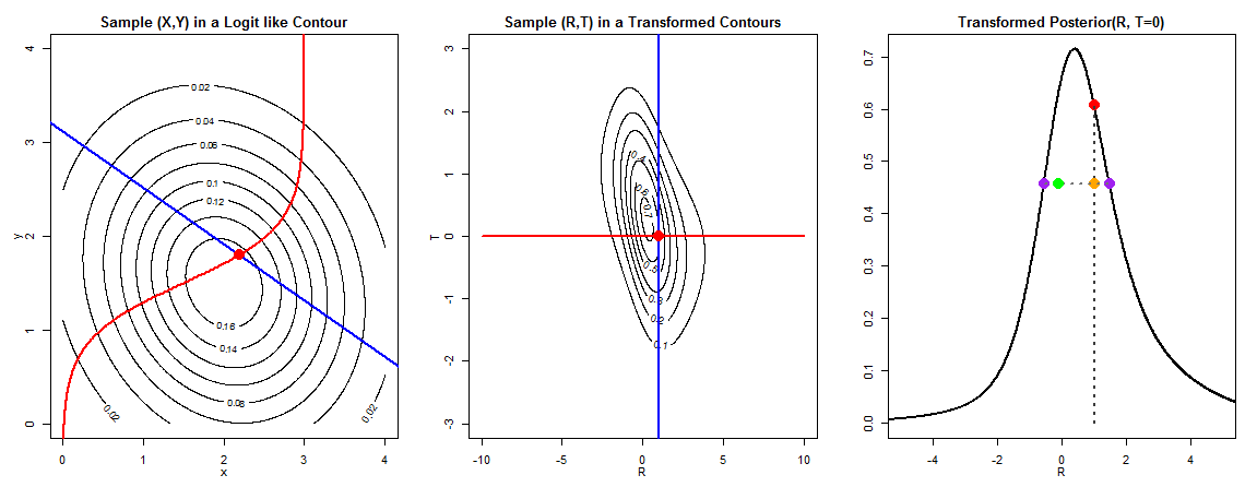
But, more crucially, we needed to modify the slice-sampler method to allow for multivariate constrained prior distributions on $\overset{{}_{\mbox{\hskip 1.42262pt}\shortleftarrow}}{R}$ and $\bm{\eta}$. Recalling that we require $\sum_{g}\eta_{g,j}=0$, we draw new samples for $\eta_{g,j}^{(t+1)}$ not by slice-sampling along the univariate density $f_{\eta_{g,j}}(\eta_{g,j}|\overset{{}_{\mbox{\hskip 1.42262pt}\shortleftarrow}}{R}^{(t)},\overset{{}_{\mbox{\hskip 1.42262pt}\shortleftarrow}}{S}^{(t)},\bm{\eta}_{,/j}^{(t)},\overset{{}_{\mbox{\hskip 1.42262pt}\shortrightarrow}}{P}^{(t)},\mathbf{Y})$ but along the full multivariate posterior density as defined along a vector, $\overset{{}_{\shortrightarrow}}{\eta}_{,j}^{(t)}(g,\Delta)$, which is perturbed by a $\frac{\Delta}{G-1}(Ge_{g}-\vec{1})$, where $e_{g}$ is the standard $g$th basis vector in $\mathbb{R}^{G}$ and $\vec{1}$ is a G-length vector of 1’s. In other words:

In this case our notation considers perturbation of a column vector $\overset{{}_{\shortrightarrow}}{\eta}_{,j}\in\mathbb{R}^{G}$ which represents all $\eta_{g,j}$ values for a single tissue-gene $j$ fixed and the crosses $g\in\{1,2,\ldots,G\}$.

To perturb $\overset{{}_{\mbox{\hskip 1.42262pt}\shortleftarrow}}{R}$, first define a logit basis reparameterization $L_{j}\equiv\log_{e}\frac{R_{j}}{1-R_{j}}$, and take a perturbation, $\frac{\Delta}{J-1}(Je_{j}-\overset{{}_{\mbox{\hskip 1.42262pt}\shortleftarrow}}{1})$, in the $\overset{{}_{\mbox{\hskip 1.42262pt}\shortleftarrow}}{L}$ logit space.

It is important to note a crucial difference in the densities used in slice-sampling of $\bm{\eta}$ versus sampling of $\overset{{}_{\mbox{\hskip 1.42262pt}\shortleftarrow}}{R}(\overset{{}_{\mbox{\hskip 1.42262pt}\shortleftarrow}}{L})$. One cannot slice-sample over arbitrary reparameterizations without changing measure. For instance, in a univariate case, if $e^{\omega}=\theta$, then, if $q_{\theta}(\theta)$ was the target density then $q_{\omega}(\omega)=q_{\theta}(e^{\omega})\times e^{\omega}$. It would be inappropriate to find the two $\omega^{+},\omega^{-}$ such that $f_{\theta}(e^{\omega^{+}})=f_{\theta}(e^{\omega^{-}})=\mbox{Unif}(0,f_{\theta}(e^{\omega^{(t-1)}}))$ and then sample $\omega^{(t)}=\mbox{Unif}(\omega^{-},\omega^{+})$. One would see a dramatically downward-biased distribution for $\theta(\omega)$. For transformations $\theta=\omega-5$ or $\theta=4\omega$, slice-sampling from $f_{\theta}(\theta(\omega))$ or $f_{\theta}(\theta)$ produces acceptably distributed samples because the linear transformation does not change the relative measure along $d\theta$.

In the multivariate setting, consider parameterization $\omega\in\mathbb{R}^{p^{\prime}}$ that transforms linearly onto the desired parameter space $\theta\in\mathbb{R}^{p}$ with $p^{\prime}\leq p$, such as $\theta=\mathbf{A}\omega+\vec{b}$. Let $\mathbf{A}_{1}$ be the top $p^{\prime}\times p^{\prime}$ square matrix of $\mathbf{A}$ and $\mathbf{A}_{2}$ be the remainder $(p-p^{\prime})\times p^{\prime}$ rectangular matrix of $\mathbf{A}$. If matrix $\mathbf{A}_{1}$ is invertible, then $\bm{\theta}_{1:p^{\prime}}$ or the first $p^{\prime}$ coefficients of $\bm{\theta}$ determine $\bm{\theta}_{(p^{\prime}+1):p}$ which are the last $p-p^{\prime}$ coefficients of $\bm{\theta}$.

If $q_{\bm{\theta}}(\bm{\theta})$ were a target density of $f_{\bm{\theta}}(\bm{\theta})$ of unknown integration constant, subject to constraints, then $q_{\bm{\theta}}(\bm{\theta})=\frac{f_{\bm{\theta}}(\bm{\theta}_{1:p^{\prime}},\bm{\theta}_{(p^{\prime}+1):p})}{\int f_{\bm{\theta}}(\bm{\theta}_{1:p^{\prime}}^{\prime},\bm{\theta}_{(p^{\prime}+1):p}^{\prime})d\theta_{1}^{\prime}\ldots d\theta_{p^{\prime}}^{\prime}}$. But also,

In Equation 8, the Jacobian $|\mathbf{A}_{1}|$ is part of the integration constant. Slice-sampling will automatically evaluate this constant.

In the case of $\overset{{}_{\shortrightarrow}}{\eta}_{,j}$, the rotation $\mathbf{A}_{1}$ is the matrix of $-1/(G-1)\vec{1}\vec{1}^{T}+\frac{G}{G-1}\mathbf{I}$ in $\mathbb{R}^{G-1}$. If $\mathbf{A}_{2}=1/(G-1)\vec{1}$ and $\vec{b}=\vec{0}$ then the reparameterized space $\overset{{}_{\shortrightarrow}}{\eta}_{,j}^{\prime}\in\mathbb{R}^{G-1}$ generates $\overset{{}_{\shortrightarrow}}{\eta}_{,j}=\{\mathbf{A}_{1}\overset{{}_{\shortrightarrow}}{\eta}_{,j}^{\prime},\mathbf{A}_{2}\overset{{}_{\shortrightarrow}}{\eta}_{,j}^{\prime}\}$ and we need not change measure.

In the case of $\overset{{}_{\mbox{\hskip 1.42262pt}\shortleftarrow}}{R}$, which includes a nonlinear transformation $\vec{L}\rightarrow\overset{{}_{\mbox{\hskip 1.42262pt}\shortleftarrow}}{R}$, the Jacobian matrix is of more consequence;

The change of variables from $\overset{{}_{\mbox{\hskip 1.42262pt}\shortleftarrow}}{R}$ to $\overset{{}_{\mbox{\hskip 1.42262pt}\shortleftarrow}}{L}$ measure is

As with $\overset{{}_{\shortrightarrow}}{\eta}_{,j}$, a linear transformation from $\overset{{}_{\mbox{\hskip 1.42262pt}\shortleftarrow}}{L}^{\prime}\in\mathbb{R}^{J-1}$, such that $\overset{{}_{\mbox{\hskip 1.42262pt}\shortleftarrow}}{L}_{1:(J-1)}=\mathbf{A}_{1}\vec{L}^{\prime}$ and $\overset{{}_{\mbox{\hskip 1.42262pt}\shortleftarrow}}{L}_{(p^{\prime}+1):p}=\mathbf{A}_{2}\overset{{}_{\mbox{\hskip 1.42262pt}\shortleftarrow}}{L}^{\prime}$, maintains the $\sum_{j}L_{j}=0$ constraint.

We note that not all $Y_{ij}$ are observed, sometimes because SNPs do not differentiate between crosses, and in other cases because of random experimental missingness. Imputation of the data missing at random is naturally accommodated in a Bayesian setting. After every iteration, the MCMC sampler draws new samples $Y_{ij}^{\mbox{\tiny{miss}}}$ missing data based upon current estimates of $P_{i}$ and $S_{j},R_{j},\eta_{g,j}$. Using these new draws of $Y^{\mbox{\tiny{miss}}}$ to make the data complete, samples of $P_{i},S_{j},R_{j},\eta_{g,j}|\mathbf{Y}^{\mbox{\tiny{complete}}}$ are drawn. When a gene is entirely excluded for a certain cross because of identical alleles, we do not impute $Y_{ij}^{\mbox{\tiny{miss}}}$ for that cross, and treat $\eta_{g,j}$ as essentially non-existent.

Because we vectorize and separate certain operations, computational costs are proportional to $\mathcal{O}(NJ)$ to update all $\overset{{}_{\mbox{\hskip 1.42262pt}\shortrightarrow}}{P},\overset{{}_{\mbox{\hskip 1.42262pt}\shortleftarrow}}{S}$ parameters, but $\mathcal{O}(NJ^{2})$ to update all $\overset{{}_{\mbox{\hskip 1.42262pt}\shortleftarrow}}{R}$ parameters and $\mathcal{O}(JGN)$ to update all $\bm{\eta}$ parameters, as well as $\mathcal{O}(G)$ to update $\overset{{}_{\shortrightarrow}}{\mu},\overset{{}_{\shortrightarrow}}{\alpha}$ parameters. Thus estimation of $\overset{{}_{\mbox{\hskip 1.42262pt}\shortleftarrow}}{R}$ seems to be the most inefficient step in the computation, where most of the computation costs come in calculation of beta values $\frac{\Gamma(R_{j}P_{i}S_{j}e^{\eta_{g,j}}+1)\Gamma((1-R_{j})(1-P_{i})S_{j}e^{\eta_{g,j}}+1)}{\Gamma((1-R_{j}-P_{j}+2R_{j}P_{j})S_{j}e^{\eta_{g,j}}+1)}$, which do not allow for the efficient separation of parameters.

Gibbs samples can be used to infer posterior mean, standard-deviation, and quantiles which we use as evidence to simultaneously test biologically relevant hypotheses, such as $\mathcal{H}_{\mu}\mbox{: }\mu_{g}=.5$, $\mathcal{H}_{S}\mbox{: }S_{j_{1}}=S_{j_{2}}$, and $\mathcal{H}_{\eta}\mbox{: }\sum_{g}(\eta_{g,j}-\bar{\eta}_{j})^{2}<10$. In particular, tests for hypotheses of the form $\mathcal{H}_{\mu_{1},\mu_{2}}\mbox{: }\mu_{g_{1}}=\mu_{g_{2}}$ are desired, and we hope to use posterior values to both defend and reject hypotheses of this type.

We can achieve roughly 50K samples in a day, and the Gelman-Rubin (Gelman and Rubin 1992) convergence measures reported in Section 5 using the complete data are quite low, so we conclude that the chain is optimized sufficiently for the purpose of testing our biological hypotheses.

Previous literature (Ruvinsky 2009; Kambere and Lane 2009; Wang et al. 2010) has suggested the alleles in Xce behave in a manner akin to a “weight-biased coin”. Consider a cross between mother carrying Xce allele “$a$” and the father with allele “$b$”. One could imagine putting a coin together with a mass $M_{a}$ for the heads face, and a mass $M_{b}$ for the tails face. If a physical model suggested $\mu(a\mbox{ $\times$ }b)=M_{a}/(M_{a}+M_{b})$, we could measure $M_{c}$ in a third allele and predict $\mu(a\mbox{ $\times$ }c)=M_{a}/(M_{a}+M_{c})$. This model is consistent with a hypothesis that Xce varies through copy number variation (CNV). Longer sequences with more copies attract nucleosomes and transcription factors to attach to the X-chromosome and deactivate it, suggesting that longer sequences at Xce are weaker alleles.

Now that we have declared multiple inbred strains of mice to carry $\mbox{\emph{Xce}}^{a}$, $\mbox{\emph{Xce}}^{b}$, $\mbox{\emph{Xce}}^{c}$, …alleles, we can implement this model within our framework. Denote the previous specification, where $\mu_{g}$ are given i.i.d. priors, our “Independence Assumption” (IA) model. After analysis, we can compare IA estimates, where no structure was assumed for $\mu_{g}$, with estimates from this weight-biased coin (WBC) model.

Consider $d(g)$ be the allele carried by the mother or “dam” for cross $g$, and $s(g)$ be the allele carried by the father or “sire” inbred-strain for cross $g$. We model $\mu_{g}$ as a function of additive allele parameters $a_{1},a_{2},\ldots,a_{K_{a}}$ for $K_{a}$ total alleles and parent-of-origin allele-specific parameters $m_{1},m_{2},\ldots,m_{K_{m}}$ for a total number of parent-of-origin alleles $K_{m}$. In our case we propose:

Having a larger $a_{d(g)}$ dam allele than the $a_{s(g)}$ sire allele pulls $\mu_{g}$ in the direction $\mu_{g}>.5$. Parent-of-origin effects $m_{d(g)}$ perturb this result based upon whether strains serve as dam or sire.

Again, we impose constraints $\sum_{k=1}^{K_{a}}a_{k}=0$ and $\sum_{k=1}^{K_{m}}m_{k}=0$. Vector-constrained slice sampling then allows for posterior sampling of these model parameters, along with the previously mentioned $\bm{\eta},\overset{{}_{\mbox{\hskip 1.42262pt}\shortleftarrow}}{R}$.

References

- Barr and Bertram (1949) Barr, M. L. and E. G. Bertram (1949). A Morphological Distinction between Neurones of the Male and Female, and the Behaviour of the Nucleolar Satellite during Accelerated Nucleoprotein Synthesis. Nature 163, 676–677.
- Bernardo and Val (1996) Bernardo, M. and U. D. Val (1996). The Concept of Exchangeability and its Applications. Far East Journal of Mathematical Science 4, 111–121.
- Brooks and Gelman (1998) Brooks, S. and A. Gelman (1998). General methods for monitoring convergence of iterative simulations. Journal of Computational and Graphical Statistics 7, 434–455.
- Calaway et al. (2013) Calaway, J., A. Lenarcic, J. P. Didion, J. R. Wang, J. B. Searle, L. McMillan, W. Valdar, and F. de Pardo (2013). Genetic architecture of skewed x inactivation in the laboratory mouse. PLoS Genetics 9(10).
- Cattanach and Isaacson (1967) Cattanach, B. and J. Isaacson (1967). Controlling elements in the mouse X-chromosome. Genetics 57(2), 331–346.
- Cattanach and Rasberry (1991) Cattanach, B. and C. Rasberry (1991). Identification of the Mus spretus Xce allele. Mouse Genome 89, 565–566.
- Cattanach and Rasberry (1994) Cattanach, B. and C. Rasberry (1994). Identification of the Mus castaneus Xce allele. Mouse Genome 92, 114.
- Cattanach and Isaacson (1965) Cattanach, B. M. and J. H. Isaacson (1965). Genetic control over the inactivation of autosomal genes attached to the X-chromosome. Molecular and General Genetics MGG 96(4), 313–323.
- Chadwick et al. (2006) Chadwick, L. H., L. M. Pertz, K. W. Broman, M. S. Bartolomei, and H. F. Willard (2006). Genetic Control of X Chromosome Inactivation in Mice: Definition of the Xce Candidate Interval. Genetics 173(4), 2103–2110.
- Chang (1983) Chang, T. (1983). Binding of cells to matrixes of distinct antibodies coated on solid surface. J Immunol Methods. 65, 17–23.
- Darvasi and Soller (1995) Darvasi, A. and M. Soller (1995). Advanced Intercross Lines, an Experimental Population for Fine Genetic Mapping. 141(3), 1199–1207.
- de Finneti (1937) de Finneti, B. (1937). Foresight: Its Logical Laws, Its Subjective Sources. Annales de l’Institut Henri Poincare 7.
- Developers et al. () Developers, R., R. A. Becker, Chambers, J. M., and A. R. Wilks. R documentation: Build shared object/dll for dynamic loading. http://stat.ethz.ch/R-manual/R-devel/library/utils/html/SHLIB.html. Accessed: 2013-09-13.
- Diaconis and Freedman (1980) Diaconis, P. and D. Freedman (1980). Finite exchangeable sequences. The Annals of Probability 8(4), 745–764.
- Efron and Morris (1977) Efron, B. and C. Morris (1977). Stein’s Paradox in Statistics. Scientific American 236, 119 – 127.
- Ferrari and Cribari-Neto (2004) Ferrari, S. and F. Cribari-Neto (2004, Aug). Beta Regression for Modelling Rates and Proportions. Journal of Applied Statistics 31(7), 799–815.
- Gelfand et al. (1992) Gelfand, A. E., A. F. M. Smith, T.-m. Lee, A. F. M. Smith, and A. E. Gelfand (1992). Bayesian Analysis of Constrained Parameter and Truncated Data Problems Using Gibbs Sampling. Journal of the American Statistical Association 87(418), 523–532.
- Gelman and Rubin (1992) Gelman, A. and D. Rubin (1992). Inference from iterative simulation using multiple sequences. Statistical Science 7, 457–511.
- Gendrel and Heard (2011) Gendrel, A.-V. and E. Heard (2011, Dec). Fifty years of X-inactivation research. Development (Cambridge, England) 138(23), 5049–55.
- Graze et al. (2012) Graze, R. M., L. L. Novelo, V. Amin, J. M. Fear, G. Casella, S. V. Nuzhdin, and L. M. McIntyre (2012, Jun). Allelic imbalance in Drosophila hybrid heads: exons, isoforms, and evolution. Molecular biology and evolution 29(6), 1521–32.
- Hall et al. (2007) Hall, D. A., J. Ptacek, and M. Snyder (2007). Protein Microarray Technology. Mech Ageing Dev. 128, 161–167.
- Hewitt et al. (1955) Hewitt, E., L. J. Savage, E. Hewitt, and L. J. Savage (1955). Symmetric Measures on Cartesian Products. Transactions of the American Mathematical Society 80(2), 470–501.
- Jackman (2009) Jackman, S. (2009). Bayesian Analysis for the Social Sciences (1 ed.). Chichester, West Sussex, UK: John Wiley & Sons, Ltd.
- Kambere and Lane (2009) Kambere, M. B. and R. P. Lane (2009, Feb). Exceptional LINE density at V1R loci: the Lyon repeat hypothesis revisited on autosomes. Journal of molecular evolution 68(2), 145–59.
- Kim et al. (2005) Kim, K., S. Thomas, I. B. Howard, T. A. Bell, H. E. Doherty, F. Ideraabdullah, D. A. Detwiler, and F. P.-m. Villena (2005). The genus Mus as a model for evolutionary studies Meiotic drive at the Om locus in wild-derived inbred mouse strains. Biological Journal of the Linnean Society 84, 487–492.
- Lawson et al. (1979) Lawson, C. L., R. J. Hanson, D. Kincaid, and F. T. Krogh (1979). Basic linear algebra subprograms for fortran usage. ACM Trans. Math. Soft. (5), 308–323.
- Lee (2011) Lee, J. (2011). Gracefully ageing at 50, X-chromosome inactivation becomes a paradigm for RNA and chromatin control. Nature Reviews Molecular Cell Biology (12), 815–826.
- Lindley and Phillips (1976) Lindley, D. and L. Phillips (1976). Inference For a Bernoulli Process ( a Bayesian View )*. The American Statistician 30(3), 112–119.
- Lindley and Smith (1972) Lindley, D. V. and A. F. M. Smith (1972). Bayes Estimates for the Linear Model. Journal of the Royal Statistical Society. Series B 34(1), 1–41.
- Lyon (1961) Lyon, M. F. (1961). Gene Action in the X-chromosome of the Mouse (Mus musculus L.). Nature 190, 372 – 373.
- Lyon (1962) Lyon, M. F. (1962, Jun). Sex chromatin and gene action in the mammalian X-chromosome. American journal of human genetics 14, 135–48.
- Mak et al. (2004) Mak, W., T. B. Nesterova, M. de Napoles, R. Appanah, S. Yamanaka, A. P. Otte, and N. Brockdorff (2004). Reactivation of the paternal x chromosome in early mouse embryos. Science 303(5658), 666–669.
- Morin et al. (2008) Morin, R., M. Bainbridge, A. Fejes, M. Hirst, M. Kryzwinski, T. Pugh, H. McDonald, R. Varhol, S. Jones, and M. Marra (2008). Whole Transciptome Shotgun Sequencing. Biotechniques 45(1), 81–94.
- Murphy (2007) Murphy, K. (2007). Software for Graphical models : a review. Isba Bulletin December, 1–3.
- Neal (2003) Neal, R. (2003). Slice Sampling Author. Annals of Applied Statistics 31(3), 705–741.
- Nishioka (1995) Nishioka, Y. (1995, Mar). The origin of common laboratory mice. Genome / National Research Council Canada = Génome / Conseil national de recherches Canada 38(1), 1–7.
- Parmigiani and Inoue (2009) Parmigiani, G. and L. Inoue (2009). Decision Theory: Principles and Approaches (1 ed.). Wiley.
- Plummer (2003) Plummer, M. (2003). JAGS : A program for analysis of Bayesian graphical models using Gibbs sampling JAGS : Just Another Gibbs Sampler. DSC 2003 Working Papers.
- Roberts et al. (2012) Roberts, G. O., J. S. Rosenthal, and S. Rosenthal (2012). Convergence of slice sampler Markov chains. Journal of the Royal Statistical Society. Series B 61(3), 643–660.
- Ronaghi et al. (1998) Ronaghi, M., M. Uhlén, and P. l. Nyrén (1998). A Sequencing Method Based on Real-Time Pyrophosphate. Science 281(5375), 363–365.
- Ruvinsky (2009) Ruvinsky, A. (2009). Genetics and Randomness. Boca Raton, FL: CRC Press.
- Sebat et al. (2004) Sebat, J., B. Lakshmi, J. Troge, J. Alexander, J. Young, P. Lundin, S. Må nér, H. Massa, M. Walker, M. C. Chi, N. Navin, R. Lucito, J. Healy, J. Hicks, K. Ye, A. Reiner, T. C. Gilliam, B. Trask, N. Patterson, A. Zetterberg, and M. Wigler (2004). LARGE-SCALE COPY NUMBER POLYMORPHISM IN THE HUMAN GENOME. Science 305(5683), 525–528.
- Shi et al. (2009) Shi, X., M. Styner, J. Lieberman, J. G. Ibrahim, W. Lin, and H. Zhu (2009, Jan). Intrinsic Regression Models for Manifold-Valued Data. Journal of the American Statistical Association 5762, 192–199.
- Stankiewicz and Lupski (2010) Stankiewicz, P. and J. R. Lupski (2010). Structural Variation in the Human Genome and its Role in Disease. Annual Review of Medicine 61, 437–455.
- Takagi et al. (1982) Takagi, N., O. Sugawara, and M. Sasaki (1982, January). Regional and temporal changes in the pattern of X-chromosome replication during the early post-implantation development of the female mouse. Chromosoma 85(2), 275–86.
- Thompson and Seber (1996) Thompson, S. K. and G. A. Seber (1996). Adaptive Sampling. John Wiley & Sons.
- Vines et al. (1996) Vines, S. K., W. R. Gilks, and P. Wild (1996). Fitting Bayesian multiple random effects models. Statistics And Computing 6, 337–346.
- Wang et al. (2010) Wang, X., P. D. Soloway, and A. G. Clark (2010, Jan). Paternally biased X inactivation in mouse neonatal brain. Genome biology 11(7), R79.
- Zho et al. (2010) Zho, H., Y. Chen, J. Ibrahim, Y. Li, C. Hall, and W. Lin (2010). Intrinsic Regression Models for Positive-Definite Matrices With Applications to Diffusion Tensor imaging. Journal of American Statistical Association 104(487), 1203–1212.
- Zhu et al. (2011) Zhu, H., J. G. Ibrahim, and N. Tang (2011, May). Bayesian influence analysis: a geometric approach. Biometrika 98(2), 307–323.