Freie Universität Berlin
Fachbereich Mathematik und Informatik
Diplomarbeit
On the Complexity of
Embeddable Simplicial Complexes
Anna Gundert
21. Oktober 2009
Betreut von Prof. Dr. Günter M. Ziegler
(Technische Universität Berlin)
Danksagung
Für die Bereitstellung des Themas, viele hilfreiche Hinweise und die Möglichkeit, Anschluß in seiner Arbeitsgruppe zu finden, möchte ich mich bei dem Betreuer dieser Arbeit Prof. Dr. Günter M. Ziegler bedanken.
Von der Arbeitsgruppe „Diskrete Geometrie“ der TU Berlin möchte ich insbesondere Ronald Wotzlaw und Raman Sanyal für ihre stetige Hilfsbereitschaft Dank aussprechen. Mein weiterer Dank gilt Mathias Schacht für das Beantworten vieler Fragen zur extremalen Hypergraphentheorie.
Desweiteren danke ich Frau Monika Seid und Frau Sandra Breiter-Staufenbiel, die in gewissem Sinne die Voraussetzungen für das Verfassen dieser Arbeit geschaffen haben, sowie meinen Eltern für ihre immer bedingungslose Unterstützung.
Zu guter Letzt möchte ich Frederik von Heymann für das gewissenhafte Lesen meiner Arbeit und ständigen Beistand danken.
Eidesstattliche Erklärung
Hiermit versichere ich, die vorliegende Arbeit selbständig und unter ausschließlicher Verwendung der angegebenen Literatur und Hilfsmittel erstellt zu haben.
Diese Arbeit wurde bisher in gleicher oder ähnlicher Form keiner anderen Prüfungskommission vorgelegt und auch nicht veröffentlicht.
Berlin, den 21. Oktober 2009 Anna Gundert
Abstract
This thesis addresses the question of the maximal number of -simplices for a simplicial complex which is embeddable into for some .
A lower bound of , which might even be sharp, is given by the cyclic polytopes. To find an upper bound for the case we look for forbidden subcomplexes. A generalization of the theorem of van Kampen and Flores yields those. Then the problem can be tackled with the methods of extremal hypergraph theory, which gives an upper bound of .
We also consider whether these bounds can be improved by simple means.
Introduction
Questions on embeddability of simplicial complexes into Euclidean space are not only connected to topology but also to combinatorics. Sarkaria’s coloring/embedding theorem (Theorem 5.8.2 [Mat03]), e.g., links the non-embeddability of a complex into Euclidean space of certain dimensions with the chromatic number of a graph associated with this complex.
The most well-studied such embeddability question is that of planar graphs, which can be considered as -dimensional simplicial complexes that allow an embedding into . Analogous questions for higher dimensions are far less understood and seem to get more complicated. Several problems that are tractable for the case of planar graphs, are far more complex and partly open in higher dimensions. Here are a few examples:
While every graph that embeds into the plane also has a straight-line embedding, there are examples of simplicial complexes of higher dimension that admit a topological embedding into some , but not a linear (or piecewise linear) embedding into this space (e.g., [Bre83], [BGdO00], [Sch06], [MTW09, p.858]). On the other hand, the planar case is not the only one in which different embeddability properties agree: It is, e.g., known that every -dimensional simplicial complex that embeds topologically into for some with is also piecewise linearly embeddable into [Bry72].
Also the algorithmic complexity of deciding whether a given -dimensional simplicial complex embeds into some is not solved for all pairs . For planarity testing polynomial algorithms have been developed. Some of the higher-dimensional cases also have polynomial complexity, in others the question is known to be NP-hard, or even undecidable [MTW09].
For the graph case it is well-known that the graphs and characterize non-planarity and are minimal non-planar graphs, i.e., all of their subgraphs are planar. The question of minimal non-embeddable complexes for higher dimensions is more complicated. While classes of such complexes are known (e.g., [Grü69], [Zak69a], [Sar91], [Sch93]), it is also known that for and no characterization via a finite set of minimal non-embeddable complexes is possible ([Umm73], [Zak69b]).
It is well-known and not hard to show that a planar graph on vertices can have at most edges. We will be interested in higher-dimensional analogues of this result, i.e., in the maximal size of complexes of dimension that are embeddable into a certain Euclidean space.
More precisely, we study the following question:
-
For fixed and , what is the maximal number of -simplices for a complex on vertices that embeds into ?
Because the complete -complex embeds into , for the maximal number of -simplices one can get when embedding a complex on vertices into is .
For the case this yields for embeddability into . One can also show that a complex which embeds into can have at most triangles. What happens in is an open question. Apart from two related conjectures ([Kal02, Conjecture 27], [Kal08]) it seems this question has not been discussed in the prior literature.
We will address the general question for . Our goal is to find lower and upper bounds. Chapter 1 will give a more detailed presentation of the problem. Chapter 2 addresses the lower, Chapter 3 the upper bounds.
We will need basic notions from quite a few areas of mathematics. Instead of explaining all necessary basic concepts in one starting chapter, I decided to introduce things whenever they are needed as we go along .
In Chapter 2 we achieve a lower bound of the order for every instance of the problem by looking at examples of embeddable complexes. These are given by the boundary complexes of polytopes. We will see that the cyclic polytopes yield the largest examples coming from polytopes, even from simplicial spheres. We then show that in the case these examples cannot be improved by simply adding further simplices.
Chapter 3 gives an upper bound for the case , where the lower bound is of the order . The smallest interesting case here is and . We approach the question of how many -simplices a complex embeddable into can have at most by looking for forbidden subcomplexes. We exclude Schild’s class of minimal non-embeddable complexes [Sch93], which seems to include all known examples of such complexes.
Turning to the methods of extremal hypergraph theory, we use a result of Erdős [Erd64] on complete -partite -graphs with partition sets of fixed size. This yields an upper bound of the order , which improves the trivial upper bound of . As Erdős’ result only estimates the extremal quantity in question, we then consider how much could be gained by a better estimate. We see that in this way the bound could not be improved to yield more than .
Chapter 1 Embedding Simplicial Complexes
This chapter introduces the main question that will be addressed in this thesis. We will first explore the notions needed to phrase the problem, namely simplicial complexes and their embeddings into Euclidean space. Then we will pose the question and discuss some first aspects.
1.1 Simplicial Complexes
Simplicial complexes are combinatorial objects that can be used to model certain topological spaces in a discrete setting. The combinatorial concept of abstract simplicial complexes has a geometric counterpart, geometric simplicial complexes: subspaces of that are built from simple building blocks. These give the connection to topology. We will only be dealing with finite simplicial complexes. Good sources for more information on this are, e.g., [Mat03] and [Mun93]. Since we will rarely consider any other types of complexes (e.g., polytopal, - or CW-complexes) the term “complex” without further specification will always refer to a simplicial complex.
Let us begin with the definition of an abstract simplicial complex.
Definition 1.1.1 (abstract simplicial complex).
Let be a finite set. An abstract simplicial complex on the vertex set is a non-empty family of subsets of that is hereditary, i.e.:
Members of are called simplices.
The dimension of a simplex is . The dimension of is . Simplices and complexes of dimension are called -simplices and -complexes respectively.
Observe that, as a simplicial complex is non-empty, it will always contain the empty set. To define the corresponding geometric concept we need some basic terminology:
Definition 1.1.2 (affine independence, geometric simplex, face).
Let .
- 1.
The set is called affinely independent if for the equations and imply that for all .
- 2.
If is affinely independent, its convex hull is a (geometric) simplex of dimension (or an -simplex). The points are the vertices of . Note that an -simplex has vertices.
- 3.
For an affinely independent set , any subset is also affinely independent and hence its convex hull is also a simplex. It is called a face of . In particular, every simplex has the empty set as a face.
The affine hull of finitely many points can be described as the set . Thus, for a set to be affinely dependent means that at least one point in , w.l.o.g. , lies in the affine hull of the others. Because this is equivalent to the linear dependence of the set , this shows that the maximal size of an affinely independent set in is . This is equivalent to asking for the affine hull of to have dimension .
Let us consider some examples of simplices: A -simplex is just a point. Any two distinct points are affinely independent. A set of three points is affinely independent if the three points do not lie on a common line. Thus, any line segment can be considered as a -simplex, a triangle as a -simplex. A -simplex is a tetrahedron, the convex hull of four points that do not lie in a common plane.

Simplices are the building blocks for geometric simplicial complexes:
Definition 1.1.3 (geometric simplicial complex).
A geometric simplicial complex in is a non-empty family of geometric simplices in that fulfills the following conditions:
- 1.
If and is a face of , then .
- 2.
If , then is a face of both and .
The dimension of a simplicial complex is ; its vertex set consists of all vertices of simplices of .

A simple example for a geometric simplicial complex is the set of all faces of a simplex , called the boundary of the simplex. Also the simplex itself can be considered as a simplicial complex: Take its boundary and add the simplex. For a -simplex, the corresponding abstract complex is simply the set of all subsets of its vertices, which is isomorphic to the power set of and is denoted by .
How are abstract and geometric simplicial complexes connected in general? A geometric simplicial complex gives rise to an abstract complex in a straight-forward way: The vertices of are just the vertices of : . A set forms a simplex of if is the vertex set of a simplex in . That means we just use the underlying set structure. For any that is isomorphic to , the geometric complex is called a geometric realization of .
In this context “isomorphic” means the following:
Definition 1.1.4 (simplicial map, isomorphism).
Let be two abstract simplicial complexes. A map between the vertex sets of the two complexes is a simplicial map from to if for all . A simplicial map from to is an isomorphism if it is bijective on the vertex sets and if its inverse is also simplicial, i.e., a map that induces a bijection between the simplices of and .
For any abstract simplicial complex with we can find a geometric realization in by identifying its vertices with the vertices of a geometric -simplex in . We can consider two geometric simplicial complexes as (combinatorially) equivalent if they are geometric realizations of isomorphic abstract complexes. With this notion, all geometric realizations of an abstract complex are equivalent, even though they might lie in surrounding spaces of different dimensions.
The union of all simplices in a geometric simplicial complex is a topological space. We will see that equivalent complexes yield homeomorphic spaces.
Definition 1.1.5 (polyhedron of a geometric simplicial complex, triangulation).
Let be a geometric simplicial complex in .
- 1.
The polyhedron of is the topological space on the set endowed with the following topology: A set is open if and only if is open in for every , where every carries the subspace topology inherited from .
- 2.
If is a topological space that is homeomorphic to , we call a triangulation of .
Note that in the case of finite complexes , which we are considering, the topology on agrees with the subspace topology inherited from .
Simple examples for spaces that admit a triangulation are the -ball, which is homeomorphic to the polyhedron of any -simplex, and the -sphere, homeomorphic to the polyhedron of the boundary of a -simplex.
With an abstract simplicial complex we can now associate for a geometric realization of . A complex might (and will) have several realizations, do these yield different topological spaces? We will see that this cannot happen: Any two isomorphic abstract complexes give rise to homeomorphic spaces.
From a simplicial map between two abstract simplicial complexes we get a map between the polyhedra of the corresponding geometric complexes:
Definition 1.1.6 (affine extension of a simplicial map).
Let and be two geometric simplicial complexes and let be the abstract complex corresponding to .
For any simplicial map from to its affine extension
is defined by
for . Here we use that every point in has a unique representation as a convex combination of the vertices of the minimal simplex in that contains it.
This map is continuous and for isomorphic complexes it is a homeomorphism:
Proposition 1.1.7 (e.g., [Mat03, Proposition 1.5.4]).
For any simplicial map its affine extension is continuous. If is an isomorphism, is a homeomorphism.
Thus, if and are two geometric realizations of the same abstract simplicial complex , the map certifies that and are homeomorphic. This shows that, up to homeomorphism, an abstract simplicial complex gives rise to a unique topological space, the polyhedron of , which we will denote by .
We can therefore stop to distinguish between abstract and geometric complexes and will from now on only talk of abstract complexes and their realizations.
We now introduce some more notions connected to simplicial complexes. In most of our considerations we will restrict our attention to complexes consisting of the faces of simplices of a fixed dimension. These are called “pure”:
Definition 1.1.8 (pure complex).
A -dimensional simplicial complex is pure if every simplex of is a face of some -simplex in . Consequently, all maximal simplices of a pure complex have the same dimension.

In what is to come we will often consider subcomplexes of simplicial complexes. One of our most important examples will be the -skeleton, a special subcomplex, of a certain complex.
Definition 1.1.9 (subcomplex, -skeleton).
Let be a simplicial complex.
- 1.
A subcomplex of is a subset of such that is also a simplicial complex, i.e.,
- 2.
For the -skeleton of is the subcomplex consisting of all simplices of dimension at most :
In addition to subcomplexes, we will also consider minors of simplicial complexes. For the definition of minors and also for several notions from piecewise-linear topology, we will need the concept of a subdivision of a simplicial complex.
Definition 1.1.10 (subdivision).
A simplicial complex is a subdivision of if there are geometric realizations and of and such that and each simplex of is contained in some simplex of .
As the last definition in this section, we will now introduce an operation for topological spaces, the join, which has certain advantages over the Cartesian product when working with simplicial complexes (e.g., [Mat03, Section 4.2]). The Cartesian product of two (geometric) simplices of dimension at least is, e.g., not a simplex, whereas the join of two simplices is. In the next section, we will encounter a family of complexes that consists of joins of certain complexes. As we will simply state results on their topological properties and only study combinatorial aspects, we now just introduce the combinatorial version of this operation: the join of two abstract simplicial complexes.
Definition 1.1.11 (join).
Let be two abstract simplicial complexes. The simplicial complex defined by the following data is called the join of and :
- •
As vertex set it has the disjoint union of the vertex sets of and :
- •
Its simplices are given by disjoint unions of simplices in and simplices in :
The disjoint union of two sets and can, e.g., be considered as the set Note that for a -complex and a -complex the dimension of the join is
1.2 Embeddings
In this section, we study embeddings of simplicial complexes into Euclidean space. We will discuss different types of embeddability and consider the minimal dimension in which a fixed complex can be embedded.
As a start remember the definition of an embedding for general topological spaces:
Definition 1.2.1 (embedding).
Let and be topological spaces.
An embedding of into is a map that is a homeomorphism onto its image . This means that with the induced topology on is bijective, continuous and the inverse function is also continuous.
In this thesis we consider embeddings of the form for -dimensional simplicial complexes . From now on, will always refer to the dimension of the complex, whereas will be the dimension of the Euclidean space in which we want to embed the complex. If embeds into we denote this by and often just say that embeds into .
Geometric realizations are of course examples of such embeddings. They can be considered as linear embeddings, where linear for a map of a simplicial complex into means that it is linear on each simplex.
A piecewise linear (PL) embedding of a simplicial complex into is a map that is a linear map of some subdivision of into as well as an embedding.

A complex that admits a topological embedding into some does not necessarily also admit a PL (or a linear) embedding into this space. In [MTW09] Matoušek, Tancer and Wagner study the computational complexity of deciding whether a given -dimensional simplicial complex embeds piecewise linearly into . They also compare linear, PL and topological embeddability; we repeat parts of their discussion here.
There are some cases where there is no difference: Every -dimensional simplicial complex that embeds topologically into for some with is also PL embeddable into [Bry72]. The same is true for and [MTW09, p.858] and also for planar graphs (i.e., -dimensional simplicial complexes that embed into ) (e.g., [Bol02, p.21]). A well-known fact from graph theory, Fáry’s Theorem (e.g., [Wes01, p.246/247]), states that for every simple planar graph there even exists a straight-line (i.e., linear) embedding.
But there are examples which show that in general these embeddability properties are not the same: There is a -dimensional complex that embeds topologically, but not PL into [MTW09, p.858]. In [Bre83] Brehm presents a -dimensional simplicial complex (a triangulated Möbius strip) that embeds into but not linearly. It has also been shown that, while trivially embedding topologically into , no triangulation of a surface of genus using only vertices admits a linear embedding in : [BGdO00] proves this for one example, [Sch06] for all. For higher dimensions, Brehm and Sarkaria [BS92] showed that for every and every such that there is a finite -dimensional complex that admits a topological but no linear embedding into . For given , it is even possible to construct such that can be embedded into , but the -th barycentric subdivision cannot be embedded linearly into .
Although our main interest will lie in topological embeddings, we will occasionally point out where our results are relevant to questions concerning the other embeddability properties.
Let us now consider the minimal dimension in which we can embed a given complex. We have already seen that a simplicial complex on vertices always has a geometric realization in . Here is a better result which depends only on the dimension of the complex, not on the number of vertices:
Theorem 1.2.2 (e.g., [Mat03, Theorem 1.6.1]).
Every finite -dimensional simplicial complex has a geometric realization in .
To prove this we will use the moment curve which will also be of use later on.
Definition 1.2.3 (moment curve).
The curve defined by
is called the moment curve in .
Lemma 1.2.4 (e.g., [Mat03, Lemma 1.6.2]).
Any distinct points on the moment curve in are affinely independent.
Proof.
To check affine dependence of points we have to solve the system of linear equations , . For points on the moment curve this leads to determining the rank of the matrix
a Vandermonde matrix. Its determinant is known to be and therefore non-zero for pairwise distinct . Thus, the zero vector is the only solution. ∎
Proof of Theorem 1.2.2.
Let be a finite -dimensional simplicial complex.
Place its vertices on the moment curve in via some . Because a simplex in has at most vertices, it corresponds to an affinely independent set. Thus, by taking the convex hulls of sets corresponding to simplices in , we get a collection of geometric simplices.
To see that this collection is a simplicial complex, we have to show that for two simplices and in the intersection of the corresponding simplices is a face of both and .
But , so the set of involved vertices is affinely independent. This means and are faces of a bigger simplex and their intersection is a face of both. ∎
Thus, every -dimensional complex can be embedded in . The following theorem by van Kampen [vK32b, vK32a] and Flores [Flo33, Flo34] shows that for some complexes this is the best possible dimension. A modern treatment can be found in [Mat03].
Theorem 1.2.5 (Van Kampen-Flores Theorem).
Let .
Then does not embed into .
More precisely, for every continuous map there exist two disjoint simplices such that .
Of course there are -dimensional complexes that can be embedded in some with . A trivial example is the -simplex which embeds into . Later we will consider (the -dimensional) boundaries of simplicial -polytopes which lie in .
We will be especially interested in -dimensional simplicial complexes that admit an embedding into . For these are planar simple graphs for which there are well-known characterizations via forbidden subgraphs and minors (e.g., [Wes01, Section 6.2]):
Theorem 1.2.6 (Kuratowski’s Theorem).
A simple graph is planar if and only if it does not contain a subdivision of or of as a subgraph.
Theorem 1.2.7 (Wagner’s Theorem).
A simple graph is planar if and only if it does not have or as a minor.
Here a minor of a graph is a graph that can be obtained from by deleting and/or contracting edges of . A subdivision of is a graph that is obtained by replacing edges of with pairwise internally-disjoint paths. With we denote the complete graph on vertices, and refers to the complete bipartite graph on two vertex sets of three elements each. (See Figure 1.5)

The graphs and are minimal non-planar graphs: All of their subgraphs are planar. Moreover, we just saw that these two graphs and all of their subdivisions are the only minimal non-planar graphs. Any other graph that does not embed into the plane contains a (proper) subgraph that is homeomorphic to one of the two and is hence non-planar.
In the case for an example of a minimal non-embeddable complex is , the complex appearing in the Theorem of van Kampen and Flores. All of its subcomplexes embed into because , where is a maximal simplex, is the complex on vertices consisting of all possible -simplices except for one. This is the -skeleton of the boundary complex of , the cyclic -polytope on vertices, as we will, e.g., see in the proof of Lemma 2.4.7.
Further classes of minimal non-embeddable complexes in higher dimensions were presented by Grünbaum [Grü69], Zaks [Zak69a], Sarkaria [Sar91] and Schild [Sch93]. Schild’s class of complexes, presented in the theorem below, contains all of these examples.
Definition 1.2.8 (nice complex).
Let be a simplicial complex on at most vertices, with a vertex set identified with some . We call nice on if the following condition holds:
The complex from the Theorem of van Kampen and Flores (Theorem 1.2.5) is one example of a nice complex: For with , the complement has elements and is thus in . In Schild’s paper the definition of a nice complex is slightly different from the definition we are using. Where we use , he instead puts , the vertex set of which is a subset of in our setting. The condition on a nice complex becomes
The only case of a complex that is nice on in which is the -simplex which Schild in his paper adds as an exception by looking at the simplex with an additional “virtual” vertex.
Here’s a short proof for this being the only case: If there exists such that , then because is nice on . This means is the only maximal simplex of .
With this definition we can now present Schild’s class of non-embeddable complexes:
Theorem 1.2.9 (Schild [Sch93, Theorem 3.1]).
Let be simplicial complexes and suppose there are such that is nice on . Then is not embeddable in for .
Except for the following two cases the complex is minimal non-embeddable, i.e., every proper subcomplex is linearly embeddable in :
- 1.
All are simplices.
- 2.
is the boundary of a simplex with an additional vertex ().
Note that this implies the statement of the Theorem of van Kampen and Flores (Theorem 1.2.5) that the complex does not embed into , as is nice on .
Can these complexes play the same role as and for planar graphs, i.e., do they describe all complexes that are embeddable in the respective dimension?
Besides the case , of planar graphs there are other classes of complexes that can be characterized by a finite set of forbidden subcomplexes or minors. Halin and Jung in [HJ64] give a characterization for -dimensional complexes that embed in by forbidden subcomplexes. A sufficient condition for embeddability of -complexes in is given in [MTW09, Corollary 5.1].
For the case and no such characterization is possible. Zaks ([Zak69b] for ) and Ummel ([Umm73] for ) showed that there are infinitely many pairwise non-homeomorphic -complexes each of which does not embed into while all of their proper subcomplexes are (even linearly) embeddable.
There is also a concept of minors for these higher dimensional cases, inspired by graph minors. In [Nev07] Nevo introduces minors for finite simplicial complexes, establishes a connection with embeddability and also shows that this concept cannot yield a characterization of embeddable graphs: He proves that for any there exist infinitely many pairwise non-homeomorphic simplicial complexes of dimension that do not embed in the -sphere while all of their proper minors are embeddable. We will introduce his concept of a minor in Section 2.4.2.
This concludes our general explorations of the embeddability of simplicial complexes. We will now turn to the question of the size of embeddable complexes.
1.3 Size of Embeddable Complexes
This section introduces the main topic of this thesis: the maximal size of complexes that are embeddable into a certain Euclidean space. More precisely, we will address the following question:
-
Let be a simplicial complex of dimension on vertices that admits a (topological) embedding into for . How many -simplices (in terms of , and ) can contain at most?
To be able to phrase the question shorter and more formally, we introduce the following notation for the numbers of simplices in a complex:
Definition 1.3.1 (-vector of a simplicial complex).
For a -complex and we denote the number of -simplices of by . The -vector of is the vector
With this we can now rephrase our question:
Problem 1.3.2.
For fixed such that and , what is (in terms of , and )
In his blog [Kal08], Gil Kalai proposes a conjecture, which he attributes to Sarkaria, concerning this question:
Conjecture 1.3.3 (Kalai, Sarkaria [Kal08]).
Let be a -dimensional simplicial complex with . Then cannot be embedded to .
The type of embeddability, linear, piecewise-linear or topological, is not specified in this conjecture. Note that, while we will be studying bounds depending on the number of vertices of a complex, here the number of maximal simplices is bounded in terms of the number of edges. Kalai also remarks that there are similar conjectures for higher dimensions. At the end of this section, we will discuss Conjecture 1.3.3 in a little more detail.
In Section 1.4 we will look into a further conjecture by Kalai and Sarkaria on the shifted complexes of embeddable complexes [Kal02, Conjecture 27] that yields a similar conjecture on this question. Problem 1.3.2 is also discussed briefly in [Mat03, Notes in Section 5.1]. A treatment of the case and , which we will study later in this section, can be found in [DE94]. The case for linear embeddings is solved in [DP98], where an upper bound for the case for linearly embeddable complexes is also presented.
We will now first explore some details of the question. Then we answer it for low values of and , where it is directly tractable, and present Dey’s and Pach’s results on the cases and for linear complexes [DP98], before we turn to a discussion of the already mentioned conjectures on Problem 1.3.2.
As a first remark, observe that, because for all simplicial complexes on vertices and all , the set
is finite, and we can thus consider its maximum.
Furthermore, note that we can restrict our attention to pure -dimensional complexes: Embeddability of a complex implies embeddability for all subcomplexes of . Thus, for any embeddable complex with the maximum number of -simplices, the pure complex
also yields an example that has the same number of -simplices.
If a simplicial complex embeds into , it can also be embedded into using inverse stereographic projection. For the converse is also true: An embedding of a -dimensional complex into some with cannot be surjective (otherwise it would be a homeomorphism between and ). So via the stereographic projection a complex that admits such an embedding can also be embedded into . This means we can (and will sometimes) consider embeddability into instead of if .
Why do we restrict the question to with ? We saw that any -complex is embeddable into . The complete -complex on vertices (with all possible simplices) thus shows that for any dimension the answer to our question is , the maximal possible one. For the complete complex does not embed into by the theorem of van Kampen and Flores. Because a -complex cannot be embeddded into , the interesting range for hence lies between and .
It is moreover sufficient to ask for to be at least , as the complete -complex on vertices is the -skeleton of the -simplex, which clearly embeds into for .
As mentioned in Section 1.2, in some cases the existence of a topological embedding implies the existence of a PL embedding: For this range is , for it is the case . In all other cases, asking for the complex to embed piecewise linearly (or linearly) and not only topologically might change the outcome of the question.
This concludes our discussion of details concerning Problem 1.3.2. After considering directly tractable cases for , , in this section, we will set out to find lower and upper bounds in higher dimensions, where the question seems to become more complicated. We present lower bounds for all instances of the problem in Chapter 2 and upper bounds for the cases in Chapter 3. As linear or PL embeddability implies topological embeddability, the upper bounds naturally also apply for the variations of the question mentioned above. The lower bounds do likewise because they come from linearly embeddable examples.
Let us now study the directly tractable cases. As examples we will use the cyclic polytopes, even though we only introduce polytopes in general and cyclic polytopes in particular in Sections 2.1 and 2.2. The face numbers of the cyclic polytopes we are using here will be calculated in Section 2.3.
Graphs
Simplicial complexes of dimension are simple graphs. As all graphs embed into , we will consider as either or . In both cases there is no difference between topological, PL and linear embeddability.
Lemma 1.3.4.
A simple graph on vertices that embeds into has at most edges.
Proof.
If a graph is embeddable into , it is a disjoint union of paths. ∎
The path of length proves this bound for to be tight. For we consider planar graphs, for which the maximum number of edges is known:
Lemma 1.3.5 (e.g., [Wes01, Theorem 6.1.23]).
A simple planar graph on vertices has at most edges.
Proof.
Let be a simple planar graph with vertices and edges.
Euler’s formula states that for any crossing-free drawing of , where is the number of faces. (A face is a maximal region of the plane which contains no point used in the drawing.)
If is connected and not a path of length 2, every face has at least edges on its boundary. Since every edge lies in the boundary of exactly two faces we get
where is the number of edges in the boundary of the -th face. With Euler’s formula this yields
If is not connected, one can simply add edges to get a connected graph with more edges but the same number of vertices. For the path of length 2 the statement is obviously true. ∎
Graphs attaining this bound are maximal planar in the sense that adding an edge will make them non-planar. All of their faces (even the outer one) are triangles.
2-Complexes
For we consider simplicial complexes that are collections of triangles and look at in the range .
Let us first consider -complexes that admit an embedding into . The -skeleton of such a complex is a planar graph. We can use our knowledge on planar graphs to attain a bound in this case:
Lemma 1.3.6.
A -dimensional simplicial complex on vertices that embeds into can have at most simplices of dimension .
Proof.
Let be a -dimensional simplicial complex that embeds into the plane. Let be the -skeleton of . In the drawing of given by the embedding, the -simplices of are among the inner faces of . Euler’s formula together with the upper bound for the number of edges gives a maximum number of (inner and outer) faces for a planar graph on vertices. Hence, we get . ∎
This bound is realized by any triangulation of the 2-simplex that has vertices and no additional vertices on the boundary. As there are complexes of this kind that embed linearly into the plane, in this case asking for linear or PL embeddings doesn’t change the outcome of the question.
The following elementary treatment of the case and can be found in [DE94]. As remarked earlier, in this case the class of PL embeddable complexes equals the class of topologically embeddable ones.
Lemma 1.3.7 (Dey, Edelsbrunner [DE94, (2.3)]).
A -dimensional simplicial complex on vertices that embeds piecewise linearly into can have at most -simplices.
Proof.
Let be a -dimensional simplicial complex on vertices with a piecewise linear embedding .
For a vertex of we can estimate the number of adjacent triangles by considering a sphere centered at . If its radius is small enough, the intersection of the sphere with the triangles (and edges) adjacent to forms a planar graph.
This graph cannot have more than vertices. Thus, by Theorem 1.3.5 it has at most edges.
This means that every vertex in is adjacent to at most triangles. Taking into account that we counted every triangle three times, we thus can see that has at most triangles. ∎
The -skeleton of the cyclic -polytopes show that this bound is tight. Again, as these are linearly embeddable complexes, in this case the answer to our question stays the same when asking for linear or PL embeddings.
The case and is the smallest for which no direct approach seems to be known. What can we say asymptotically about the maximal number of triangles among all -complexes that embed in ? The complete complex yields the trivial upper bound of in this case.
3-Complexes
We will only present a direct treatment of the case of -complexes that admit a PL-embedding into . The idea that yielded an upper bound for -complexes in can be used to deal with this case:
Lemma 1.3.8.
A -dimensional simplicial complex on vertices that embeds piecewise linearly into can have at most simplices of dimension .
Proof.
Let be a -complex with a piecewise linear embedding , and a vertex of . We can again consider a small enough sphere around the vertex . As above, the -skeleton of yields a planar graph on the sphere. Every tetrahedron of containing corresponds to a face of . Thus, .
To get a more precise bound, we can use the fact that there are at least four outer vertices of , i.e., vertices for which any neighborhood of contains points not in . For these vertices at least one face of the planar graph does not correspond to a tetrahedron of . So what we get is:
∎
This bound is attained by the boundary complex of the cyclic 4-polytope minus a facet, which admits a linear embedding into . For Problem 1.3.2 thus has the same answer for linear and for PL embeddable complexes.
This concludes the discussion of the easily approachable cases. All results are summarized in Table 1.1.
∗ This holds for -complexes that PL-embed into .
Linear embeddings of -complexes in and
In [DP98] Dey and Peach treat the cases and for linear embeddings with elementary methods. They prove more general statements; we now state their results in a reduced version.
Theorem 1.3.9 ([DP98, Theorem 2.1]).
One can select at most -dimensional simplices induced by points in with the property that no of them share a common interior point. This bound cannot be improved.
Theorem 1.3.10 ([DP98, Theorem 3.1]).
Let be a family of -simplices induced by an -element point set such that no members of have a common interior point. Then .
As two maximal simplices of a simplicial complex are not allowed to share a common interior point, these upper bounds apply to the class of simplicial complexes with geometric realizations in , resp. .
The example showing the asymptotic tightness in the proof of Theorem 1.3.9 is a simplicial complex. Actually, it is the same example that will give us our lower bound in Section 2. Hence, the tightness also holds for simplicial complexes:
The bound in Theorem 1.3.10 is asymptotically tight for , as we saw in Lemma 1.3.7 above. For we will see a lower bound of order .
1.4 Algebraic Shifting and the Kalai-Sarkaria-Conjecture
Before we address the questions of lower and upper bounds, we now present a conjecture by Kalai and Sarkaria on shifted complexes which implies a conjecture concerning Problem 1.3.2 and also examine Conjecture 1.3.3 a little closer.
Let us first look at Conjecture 1.3.3. First, note that the bound on the number of triangles in this conjecture can be rephrased as a bound on the average number of triangles per edge: Let denote the number of edge-triangle incidences in a complex , i.e., . Then the condition is equivalent to asking for
The -skeleton of the boundary of the cyclic -polytope shows that strengthening the conjecture by asking for with is not possible: For we have that embeds into and that
which shows that for every and large enough.
Originally, Kalai had also proposed a stronger version of this conjecture, which would apply to if it satisfies .
The following example, found by Raman Sanyal and myself, contradicts the strengthening: The boundary of a bipyramid over a triangle with the missing triangle added has vertices, edges and triangles and thereby fulfills the strengthened inequality. At the same time it is clearly embeddable into and, indeed, into . (See Figure 1.6.)

A further conjecture concerning Problem 1.3.2 can be derived from a conjecture by Kalai and Sarkaria on shifted complexes. To phrase this statement we first need to learn a little bit about algebraic shifting, a prominent tool in -vector theory. More details on and references to proofs for the results stated here can be found in [Kal02] and [BK88].
Definition 1.4.1 (shifted complex).
A simplicial complex on the vertex set is called shifted if for any , and we also have .
This means in a shifted complex we can exchange any vertex of a simplex with a “smaller” one and still get a simplex of the complex.
There are several shifting operations which assign to a simplicial complex a shifted complex with the same -vector as . Algebraic shifting, introduced by Kalai [Kal84, Kal85], is based on algebraic constructions. It preserves not only the -vector but among other topological properties also the Betti-numbers (i.e., the ranks of the homology groups) of the complex. Since every shifted complex is homotopy equivalent to a wedge of spheres, no shifting operation can preserve the homotopy type in general.
Algebraic shifting comes in two versions: exterior and symmetric algebraic shifting. For both operations, the resulting shifted complexes and of a simplicial complex depend on the characteristic of the field that is used in the construction. These two operations do not coincide: For a simplicial complex the shifted complexes and are generally not the same.
The conjecture we are interested in involves , the boundary complex of the cyclic -polytope , which we use here again before defining it in Section 2.2. For this complex, exterior and symmetric algebraic shifting coincide and the shifted complex is the complex that is defined as follows (see [Kal91] for symmetric, [Mur07] for exterior shifting):
Definition 1.4.2 ().
The pure -dimensional simplicial complex with vertex set and the set of maximal simplices
is denoted by .
Kalai and Sarkaria independently stated the following conjecture:
Conjecture 1.4.3 (Kalai, Sarkaria [Kal02, Conjecture 27]).
If a simplicial complex on vertices admits an embedding into , then .
The type of algebraic shifting, exterior or symmetric, is not specified in [Kal02]. Because shifting preserves -vectors, it follows from that for all . Thus, the above conjecture would immediately imply the following:
Conjecture 1.4.4.
Let such that and let . Let furthermore be a -complex on vertices that embeds into .
Then has at most as many -simplices as , the boundary complex of the cyclic ()-polytope with vertices. Moreover, for all . Thus,
Note that the combinatorial constraints on the complexes in Conjecture 1.4.4 and Conjecture 1.3.3 are not equivalent: For a -dimensional simplicial complex on vertices that admits an embedding into , Conjecture 1.4.4 would yield
This does neither directly imply nor directly follow from .
Lemma 1.4.5.
If is -dimensional and shifted, then
Proof.
We first determine the set of -simplices of . A maximal simplex of is a set with , satisfying the following constraints:
The set of maximal simplices of is hence
where we write for the set . It follows from this that has the following -simplices:
where, again, denotes the set .
Now let be a shifted subcomplex of . Every -simplex of is of the form with and . If denotes the set of -simplices of and the set of edges, we consider the map that maps the -simplex to the edge , which is in because is in . A fixed edge in is the image of at most four -simplices. Hence, .
Because is shifted and contains some -simplex, the simplex and with it the edges and are in . The map doesn’t map any -simplex to these two edges. This shows that
∎
If Conjecture 1.4.3 would hold, a -complex admitting an embedding into would satisfy , and hence
To see that the combinatorial constraint on the complexes from Conjecture 1.3.3 does not imply the statement of Conjecture 1.4.3 consider the simplicial complex . This complex is shifted and fulfills
where the second inequality holds by Lemma 1.4.5 and the third because we have .
Chapter 2 Lower Bounds
This chapter will be devoted to finding lower bounds for all instances of Problem 1.3.2. We first introduce polytopes in general and, as an example, the aforementioned cyclic polytopes. We will see that certain polytopes can be used as examples of embeddable complexes and that the cyclic polytopes have maximal -vectors among them. These will then yield the promised lower bound. For the case we afterwards consider why this bound cannot be improved by simple means.
2.1 Polytopes
Convex polytopes are geometric objects with a lot of underlying combinatorial structure. Spanning a whole area of mathematics, they are interesting on their own right and are not treated fairly when just considered as examples of simplicial complexes. But as this is the focus of this thesis, we will have to make do with a very short introduction into the topic of convex polytopes, focusing on their combinatorial aspects, especially, of course, on the numbers of faces, and possible embeddings. We will mainly follow [Zie98].
Let us begin with the definition of a convex polytope. We will from now on just speak of “polytopes” as we will not consider non-convex polytopes.
Definition 2.1.1 (polytope).
A polytope in is the convex hull of finitely many points in . The dimension of is the dimension of its affine hull. If is -dimensional it is called a -polytope.
This tells us that we already saw examples of polytopes: -simplices, which are convex hulls of points in for . The -cube is another elementary example of a polytope. It is the convex hull of all points with -coordinates in . Further examples are the cyclic polytopes which we will consider in the next section.
A major basic theorem in polytope theory states that a polytope can equivalently be defined as a bounded intersection of a finite family of closed halfspaces in some (e.g., [Zie98, Theorem 1.1]). Here, “bounded” means not containing any ray of the form .
We will now define the faces of a polytope which connect the geometric object with a combinatorial structure.
Definition 2.1.2 (face of a polytope).
Let be a polytope in . If is a hyperplane for which lies entirely in one of the halfspaces determined by , the intersection of and is called a face of . The intersection of with the entire space , i.e., itself, is also considered as a face of . All other faces are referred to as proper faces.
For every polytope it is possible to find a hyperplane that doesn’t intersect . Thus, the empty set is a face of every polytope.
One can also quickly see that every face of is itself a polytope: Let be a hyperplane defining . Then is the intersection of with the halfspace determined by that does not contain entirely and hence an intersection of finitely many halfspaces.
Thus, we have a notion of dimension for the faces of a polytope. Faces of dimension are referred to as vertices. A -dimensional face of a -polytope is called a facet.
One can also show the following basic properties of faces of polytopes:
Proposition 2.1.3 ([Zie98, Proposition 2.2, Proposition 2.3 and Exercise 2.4]).
Let be a polytope.
- •
Let be the set of vertices of . Then .
- •
If is finite and , then contains the vertices of .
- •
Every proper face of is contained in a facet of .
- •
For a face of , every face of is also a face of .
- •
The intersection of two faces of is again a face of .
Let be a polytope for which all proper faces are simplices. The last two statements in Proposition 2.1.3 show that the set of all proper faces of is then a simplicial complex. Polytopes with this property are called simplicial:
Definition 2.1.4 (simplicial polytope).
A polytope is simplicial if every facet of is a simplex.
Note that, as all faces of a simplex are again simplices, by Proposition 2.1.3 it is enough to ask for the facets of to be simplices. See Figure 2.1 for an example of a simplicial and a non-simplicial polytope.

We will be interested in simplicial polytopes with an additional property, neighborliness. The Upper Bound Theorem, which we will consider in more detail in Section 2.2, states that these have maximal numbers of faces.
Definition 2.1.5 (neighborly polytope).
A polytope is -neighborly if any subset of at most of its vertices is the vertex set of a face of . A -neighborly -polytope is also just called neighborly.
The -simplex, e.g., is -neighborly. It is not hard to see that any other polytope can be at most -neighborly (e.g., [Grü03, Section 7.1]). The cyclic polytopes will turn out to be examples of neighborly simplicial polytopes.
The set of proper faces of a polytope always forms a sort of complex; it might just not consist of simplices, but of other polytopes. There is a generalization of the concept of simplicial complexes capturing this situation:
Definition 2.1.6 (polytopal complex).
A polytopal complex in is a non-empty family of polytopes in with:
- 1.
If and is a face of , then .
- 2.
is a face of both and .
The dimension of a polytopal complex is . The set is called the underlying set of .
With a polytope we can associate , the boundary complex of , which consists of all proper faces of and by Proposition 2.1.3 is a polytopal complex. Of course itself can also be considered as a polytopal complex. As remarked earlier, for simplicial polytopes the boundary complex is a simplicial complex.
To be able to compare and equate polytopal complexes we need a concept of equivalence:
Definition 2.1.7 (combinatorial equivalence).
Two polytopal complexes are combinatorially equivalent if there exists a bijective map such that if and only if for .
Note that this notion is a generalization of the concept of isomorphisms for simplicial complexes: A bijective simplicial map with simplicial inverse induces a map like this on the simplicial complexes.
By interpreting a polytope as a polytopal complex consisting of all of its faces, one gains from this definition a notion of combinatorial equivalence for polytopes. For polytopes (and also for polytopal complexes) there is also a second, geometric notion of equivalence: Two polytopes and in and respectively are affinely isomorphic if there is an affine map such that is bijective onto .
Observe that this is a stronger notion: While the existence of an affine isomorphism implies combinatorial equivalence, two combinatorially equivalent polytopes do not have to be affinely isomorphic. Any affine isomorphism maps, e.g., the square , which is combinatorially equivalent to any -polytope with vertices, onto a parallelogram. As we are more interested in the combinatorial aspects of polytopes, we will use the combinatorial concept.
Before we move on to the introduction of cyclic polytopes we will now consider the embeddability of the simplicial complexes that arise from simplicial polytopes.
Let be a -polytope. Like every -polytope, can be embedded into . By projecting from an inner point of onto a surrounding sphere, one can see that the underlying set of is homeomorphic to a -sphere. Thus, if we take out a facet (even one point would be enough, but we want to maintain the structure of a complex), the stereographic projection maps homeomorphically onto some subset of .
Another way to see this, which even yields a linear embedding, is via the technique of Schlegel diagrams (e.g., [Zie98, Chapter 5]). This gives us the following result:
Theorem 2.1.8 (e.g., [Zie98, Proposition 5.6]).
For every -polytope and every facet of there exists a polytopal complex in that is combinatorially equivalent to .
In summary, the main result of this section is that we can get examples for embeddable complexes from simplicial polytopes: For a simplicial -polytope and every facet of we have the simplicial complex . This complex is isomorphic to a (geometric) simplicial complex in and thus admits a linear embedding into .
2.2 The Cyclic Polytopes and the Upper Bound Theorem
In this section, having mentioned them several times already, we finally introduce cyclic polytopes. After seeing their definition and some of their properties, we will encounter the promised Upper Bound Theorem which states that for every , the cyclic -polytope on vertices has the maximal number of -faces among all -dimensional polytopes with .
To define cyclic polytopes we need to recall the definition of the moment curve, introduced in Section 1.2. For and , let be the moment curve in , i.e., , and choose . What can we say about the polytope ?
We saw in Lemma 1.2.4 that no distinct points on can lie in a common hyperplane. This immediately tells us two things: Firstly, the affine hull of must be all of because . This makes a -dimensional polytope.
Furthermore, as a facet is the intersection of with a hyperplane, no facet of can contain more than points of . A facet, as a -polytope, has to have at least vertices which by Proposition 2.1.3 have to be among the . Thus, every facet of has affinely independent vertices and is hence a simplex. This shows that is a simplicial -polytope. With a little more effort one can say much more about the combinatorial properties:
Theorem 2.2.1 (Gale’s Evenness Condition, e.g., [Zie98, Theorem 0.7]).
Let , , choose and set
Identify with and choose with . Then the following two statements are equivalent:
- 1.
is the vertex set of a facet of .
- 2.
For all with the number of between and is even.
This tells us for example that the vertex set of is : For every one can find a set such that satisfies the evenness condition. Thus, every is contained in a vertex set of a facet of and is hence a vertex of .
Actually, Gale’s Evenness Condition determines the complete combinatorics of , independently of the choice of parameters , which justifies the following definition:
Definition 2.2.2 (cyclic polytope).
For and , the notation refers to any member of the combinatorial equivalence class of for some choice of parameters . We call the cyclic -polytope on vertices. Its vertex set is identified with by .
The evenness condition can easily be extended to describe all proper faces of (e.g., [Zie98, Exercise 0.8]), which then shows that the cyclic polytope is neighborly, i.e., that any subset of at most vertices forms the vertex set of a face.
We already mentioned before that, for all , the cyclic polytope has the maximal number of -faces among all -polytopes on vertices. This result is known as the Upper Bound Theorem for polytopes. For us this means that cyclic polytopes will yield the best examples we can obtain from polytopes.
To be able to phrase the theorem more compactly, we first introduce a notation for the numbers of faces of a polytope. Just as for simplicial complexes this is the -vector of a polytope:
Definition 2.2.3 (-vector of a polytope).
The -vector of a -dimensional polytope is the vector where denotes the number of -faces of .
Note that for some purposes it is convenient to add , corresponding to the empty face, as first entry of the -vector. For our intentions this is not necessary.
Theorem 2.2.4 (Upper Bound Theorem, e.g., [Zie98, Theorem 8.23]).
Let be a -polytope on vertices and let . Then can have at most as many -faces as the cyclic polytope : .
If for some with , then is neighborly.
The first complete proof of the Upper Bound Theorem for all polytopes was given by McMullen [McM70]. McMullen’s proof, also given in [Zie98], which involves deeper results of polytope theory than we have at hands, also shows that all simplicial neighborly -polytopes on vertices have the same -vector as and yields the exact number of faces:
Proposition 2.2.5 (e.g., [Zie98, Corollary 8.28]).
Let be a simplicial neighborly -polytope with vertices and let .
Then , where
That the Upper Bound Theorem holds is known not only for polytopes, but also for several classes of simplicial complexes, see, e.g., [Nov03] for a list of such classes. Stanley proved that it holds for all simplicial spheres, i.e., simplicial complexes that have a triangulated sphere as geometric realization ([Sta75], also see chapter II.3 in [Sta96]). This means that
if is a simplicial complex with and . This really is a stronger statement than Theorem 2.2.4 as not all triangulations of spheres are polytopal; actually most are not [Kal88].
2.3 A Lower Bound via Simplicial Polytopes
The last sections showed that simplicial polytopes yield examples of simplicial complexes which are embeddable into a certain Euclidean space and that the neighborly ones among them, in particular the cyclic polytopes, will give maximal -vectors. We will now apply these insights to Problem 1.3.2. Recall that we are interested in the maximal number of -simplices for a -dimensional simplicial complex on vertices that embeds into for some . Theorem 2.1.8 and Proposition 2.2.5 yield the following lower bound for this:
Proposition 2.3.1.
Let such that and let . Then
These bounds can be attained by simplicial complexes that admit a linear embedding into . For the case , the same asymptotic lower bound also holds for embeddability into :
Proof.
First, consider the case . The results of the last two sections show that the complex is a -dimensional simplicial complex on vertices which, by Theorem 2.1.8, admits a linear embedding into .
By Proposition 2.2.5 the number of -simplices of is
For the case consider for some facet of . embeds linearly into and has
-simplices. The complex embeds into and has one more simplex. ∎
Note that Conjecture 1.4.4 together with Proposition 2.3.1 would imply that is the solution to Problem 1.3.2. As the complexes yielding the lower bound in Proposition 2.3.1 embed linearly and any upper bound for the problem on topological embeddability also applies for the linear version of the question, this would also mean that the answer to Problem 1.3.2 doesn’t change when considered for linear or PL embeddable complexes.
In Section 1.3 we considered Problem 1.3.2 for several low values of and . For and , we already referred to the cyclic polytope as an example attaining the presented upper bounds. Now, we can see that it actually has
faces of dimension and
-simplices.
As remarked, the case and seems to be the simplest that is yet unsolved. Here we consider the complex for which we can calculate in a similar fashion that it has triangles, a fact we already used when discussing the different conjectures concerning Problem 1.3.2. For this case, we thus get a lower bound of . The trivial upper bound given by the complete complex in this case is . In the forthcoming sections we will see that it is not possible to push up the lower bound by adding further -simplices to while preserving embeddability into . Furthermore, the chapter on upper bounds will present an upper bound of which slightly improves the trivial bound but is still far from this lower bound.
For the more general case the complex yields a lower bound of . For all these cases we will show in the remainder of this part on lower bounds that the examples given by neighborly simplicial polytopes cannot be improved in the fashion described above.
The Upper Bound Theorem shows that this is the best lower bound we can achieve by considering simplicial polytopes, and also simplicial spheres in general, as examples of embeddable complexes.
2.4 Improving the Lower Bound (for the Case )?
In the previous section we attained a lower bound for the maximal number of faces of a complex that is embeddable into a certain Euclidean space by presenting the boundary complex of the cyclic polytope as an example of such a complex. Now we want to study whether this bound can be improved by adding further simplices to the complex without adding new vertices and such that it still stays embeddable into .
For the cases we will show that this is not possible. First, we will present a theorem that considers this situation in a more general context and gives the negative answer for our case. Then we will try to see more directly why the embeddability is destroyed when adding an additional simplex, by looking for subcomplexes and minors of which we know that they are not embeddable.
The methods we will you use do not apply for the cases where , hence the question remains to be answered for these cases.
2.4.1 Adding Missing Faces to Skeleta of PL-Spheres
Consider the following theorem by Nevo and Wagner:
Theorem 2.4.1 (Nevo, Wagner [NW08, Theorem 1.2]).
Let be a piecewise linear -sphere and a missing -face of . Then does not embed into .
To see why this theorem captures our situation, we first have to explain some of the terms that appear in the theorem.
- •
Let be a -subset of the vertices of a simplicial complex . We call a missing -face of if is not contained in but its boundary is: , .
- •
Two simplicial complexes are piecewise linearly homeomorphic (PL-homeomorphic) if they have subdivisions that are isomorphic as simplicial complexes. A piecewise linear -sphere (PL--sphere) is then a simplicial complex that is piecewise linearly homeomorphic to .
A PL--sphere thus has a subdivision that is isomorphic to some subdivision of . (See [Lic99] for an introduction to piecewise linear topology.)
Let us now check whether we have the right ingredients for Theorem 2.4.1: The complex is a piecewise linear -sphere because any simplicial subdivision of the boundary of an -polytope is PL-homeomorphic to (e.g., [Lic99, Lemma 4.2]) and thus a PL--sphere.
Furthermore is -neighborly, which means that its boundary complex contains all possible -simplices. So any -subset of that is not the vertex set of a -simplex of is a missing -face.
And, as mentioned before, for a -complex embeddability into is equivalent to embeddability into . Therefore, this theorem yields that the complex does not admit an embedding into for any -set that is not the vertex set of a -face of .
This reasoning obviously works for any simplicial neighborly polytope:
Corollary 2.4.2.
Let be a simplicial neighborly -polytope and let be a set of vertices of that does not correspond to a -face of . Then does not embed into .
Of course this doesn’t mean that one could not get a bigger complex than by starting off with a non-neighborly simplicial polytope (or simplicial sphere) with less -faces and adding “non-missing” non-faces to it.
Since not all simplicial spheres are piecewise linear (e.g., [Lic99], p.302), the most general statement we can achieve for our purposes with similar reasoning is the following:
Corollary 2.4.3.
Let be a -dimensional simplicial complex on vertices that admits an embedding into and assume, furthermore, that there exists a subcomplex with such that for some neighborly PL--sphere . Then and .
Note that neighborliness for simplicial complexes has exactly the same meaning as for polytopes.
In [NW08] Nevo and Wagner conjecture that Theorem 2.4.1 holds for general simplicial spheres. For our question, this would mean that no example coming from a neighborly simplicial sphere, also not the ones coming from non-PL-spheres, can be extended to yield a higher bound than .
For the other cases, when , Theorem 2.4.1 doesn’t answer our question: The complex is a piecewise linear -sphere, but to apply Theorem 2.4.1 we first of all need to be even. Furthermore we have to add some missing -face by adding the additional -simplex.
For even , the complex is -neighborly, which means that any -subset of that is not the vertex set of a -simplex is a missing -face. Thus, if the boundary of the -simplex that we want to add to does not contain all possible -simplices, adding the -simplex would also mean adding a missing -face. But for general even , not all -faces of have this form: , for example, has missing 3-faces.
2.4.2 An Elementary Approach
Is it possible to see directly why adding an additional simplex makes the complex no longer embeddable into ?
One possibility would be to find in the resulting complex a subcomplex of which we know that it is not embeddable. In Section 1.2 we saw examples of non-embeddable complexes: the joins of nice complexes (Theorem 1.2.9). They will be studied more deeply in an upcoming section.
Let us consider the case . In Section 3.3 we will see that there are only three possibilities for a join of nice complexes where the dimension of the complex is and the dimension of the Euclidean space is (Lemma 3.3.3). These complexes are
- •
(the threefold join of the complex consisting of only three vertices, i.e., the join of the complete bipartite graph with the complex consisting of three vertices),
- •
(the join of the complete graph with the complex consisting of three vertices) and
- •
(the -skeleton of the -simplex, i.e., all possible triangles on vertices).

We will now see that these do not have to appear when an additional -simplex is added to the -skeleton of a cyclic -polytope. This shows that as subcomplexes the non-embeddable complexes from Theorem 1.2.9 do not yield a clearer picture of the non-embeddability of for a missing -face .
Lemma 2.4.4.
There is a missing -face of such that the complex contains none of the three complexes , and as a subcomplex.
Proof.
Let us first consider which sets with are not a vertex set of a -face of . By Proposition 2.1.3 this is the case if and only if there is no facet of that contains the vertices and .
By Gale’s Evenness Condition a set with corresponds to a facet of if and only if for all with the number of between and is even. This means that all maximal intervals in that contain neither nor have even length, where “maximal interval” refers to a set for which neither nor are subsets of .
We will now check when a set with can be extended to such a -set . Let us for the moment call an element of a set isolated if , and . If there is no isolated vertex in , it is possible to add two additional vertices such that the resulting set satisfies the above criterion for a facet. Also if only one or two of , and are isolated, we can add neighbors of the isolated vertex or vertices to create a facet. These cases occur precisely if or or at least two of are adjacent.
If all three vertices , and are isolated, we would need at least three additional vertices to make all maximal intervals not containing or have even length. This shows that is not a -face if and only if , and are isolated, i.e., if and .
The complete list of missing 2-faces of is therefore (with written as ):
Remember that every set that does not correspond to a -face of our polytope is a missing -face as the neighborly polytope has a complete -skeleton.
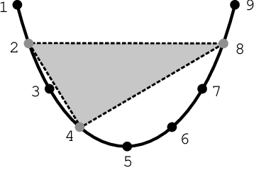
We will now show that does not contain any of the three non-embeddable subcomplexes:
-
The nine vertices of this complex are partitioned into three sets of three vertices each, such that the complex contains precisely those -sets that have one vertex in each of the three sets.
For to be one of the simplices, each of the three sets would hence have to contain one of the vertices and . In which of the sets could we then put the vertex ? (We have to use all vertices!) Because and are missing, cannot be contained in any of the three sets.
-
This complex has eight vertices, partitioned into one set of five and another set of three vertices. The simplices are exactly the sets that contain two vertices in and one in .
We thus have to have and .
The vertex cannot be a vertex of the subcomplex: If it was, it would have to form a simplex with two of the vertices and . The missing faces and prevent this.
This means we have to use all other vertices: and . We distinguish two cases:
-
Because is missing, has to be in the same partition set as . The same is true for and (). This means that and are not in the same set ( and are not!). So would have to be a simplex!
-
Then and, because of the missing faces and , we would have . This would mean that and thus . But then would have to be a simplex!
-
To find this complex as a subcomplex of , we have to choose four further vertices such that is the only missing -face on these seven vertices. Because and are missing, we cannot pick or . This leaves us with the seven vertices and . But is also not a face of .
This shows that does not contain any of the three complexes , and as a subcomplex. ∎
So we see that, when trying to understand why for a missing -face is not embeddable, it doesn’t suffice to consider the non-embeddable complexes from Theorem 1.2.9 as subcomplexes.
We can, however, use a concept of minors for simplicial complexes to gain more insight into the non-embeddability of these complexes. As already mentioned in Section 1.2, Nevo introduces a notion of minors for finite simplicial complexes and explores their connection with embeddability in [Nev07].
This is his definition of a minor:
Definition 2.4.5 (minor).
Let and be simplicial complexes.
- •
If is a subcomplex of , the operation of replacing by is called a deletion.
- •
If is obtained from by identifying two distinct vertices that are not contained in any missing -face of with , the operation of replacing by is called an admissible contraction. See Figure 2.4 for an example. If are identified, the resulting complex is
We call a minor of if can be obtained from by a (finite) sequence of admissible contractions and deletions. We denote this situation by .

Nevo proves, among other things, the following statement about the -skeleton of the -simplex which, by the Theorem of van Kampen and Flores (Theorem 1.2.5), does not allow an embedding into and is also contained in the class of non-embeddable complexes of Theorem 1.2.9.
Theorem 2.4.6 (Nevo [Nev07, Corollary 1.2]).
For let be a simplicial complex such that . Then cannot be embedded into .
We now apply this to our question by showing that adding an additional simplex to creates as a minor and thus destroys embeddability into . [NW08, Remark 6.4] states this without proof. Note that this proof of the non-embeddability of for a missing -face is independent of Theorem 2.4.1.
Lemma 2.4.7.
Let be a missing -face of for . Then is a minor of .
Proof.
Let us first identify the missing -faces of . By Gale’s Evenness Condition and Proposition 2.1.3 we know that with is a -face if and only if there are additional vertices such that these vertices are arranged in one block of odd length containing either or and possibly several blocks of even length. Phrased with the terminology from the proof of Lemma 2.4.4 this means that the maximal intervals formed by these vertices that do not contain or are of even length.
It follows from this that is a -face if and only if , or it contains two adjacent vertices , as these are the cases when there are vertices that might need a neighbor. Thus, for our missing face we have with , and for . Again with the terminology of Lemma 2.4.4 this means that all elements of are isolated vertices.

Let . By the above arguments, for there is no missing -face of containing the vertices and . Because is -neighborly, this means that identifying two vertices with , if such vertices exist, is an admissible contraction in .
Let us now look at the resulting complex . Just like it contains all possible -simplices for . Which -simplices are in ? Certainly all -simplices of not containing remain. Of the others, the ones that have and as elements turn into -simplices. The ones that do not contain become -simplices of the new complex, now containing instead of .
This means for with we get
which proves that is isomorphic to the -skeleton of the cyclic -polytope on vertices with as an additional simplex.
We can proceed to contract vertices in this manner until there is no more such that , and . This is the case if we are left with vertices and our missing face contains every second vertex.
Thus, it suffices to consider the case and where is the only missing -face and hence the complete complex on vertices: . ∎
This concludes the part on lower bounds. We achieved a lower bound by looking at the cyclic polytopes as examples of embeddable complexes and could see that these examples cannot be improved by just adding more simplices.
Chapter 3 Upper Bounds
In this chapter, we now turn to upper bounds for Problem 1.3.2. The idea we will pursue is to exclude certain non-embeddable complexes as subcomplexes. In Section 1.2 we already introduced a class of complexes, which seems to contain all known examples of minimal non-embeddable complexes. We will recall their definition in Section 3.3. A complex that has such a complex as a subcomplex is itself non-embeddable. Thus, if a certain number of simplices enforces these complexes as subcomplexes, it also enforces non-embeddability.
To this end, we will consider simplicial complexes as hypergraphs, a generalization of graphs which will be introduced at the start of this chapter. We will then use results from extremal hypergraph theory to estimate the number of edges that enforces as subgraphs the hypergraphs corresponding to our forbidden complexes. We only get a result for certain instances: We show that for large enough , a -dimensional simplicial complex on vertices that embeds in can have at most -simplices, which slightly improves the trivial upper bound of .
In the last part we will see that a better estimate for the number of edges enforcing these forbidden subgraphs could not improve this bound by much.
3.1 Hypergraphs
We start by quickly introducing hypergraphs. While edges of a graph always contain exactly two vertices, the edges of a hypergraph are arbitrary subsets of the set of vertices:
Definition 3.1.1 (hypergraph).
A (finite) hypergraph is a pair where is a finite set and is a collection of subsets of : . Elements of are called vertices; the edges of are the elements of . We will denote the number of vertices of a hypergraph by and its number of edges by .
A subhypergraph of a hypergraph is a hypergraph with and .
Note that the edges of a hypergraph can have different cardinalities. Hypergraphs where all edges have the same cardinality are called regular:
Definition 3.1.2 (-regular, -graph).
Let . A hypergraph is -regular or simply a -graph if all of its edges have cardinality : for all .
The objects of standard graph theory could, e.g., in this context be referred to as 2-graphs. We will continue calling them graphs where there is no ambiguity.
Comparing hypergraphs and abstract simplicial complexes ,which are also collections of subsets of some vertex set, one can observe one difference: Simplicial complexes are hereditary, i.e., for each edge they also contain all of its subsets. Hypergraphs don’t have to be: a hypergraph could for example contain a “triangle” along with the edge but not the other two edges. One could consider simplicial complexes as (non-regular) hereditary hypergraphs. Pure -dimensional simplicial complexes are in one-to-one correspondence with -graphs: The set of all -simplices of a pure -dimensional complex , denoted by , is the edge set of a -graph, and by adding all subsets of edges we can regain from it.
We will mostly be interested in -regular hypergraphs with an additional property, a generalization of bipartite (2-)graphs:
Definition 3.1.3 (-partite -graph, complete -partite -graph).
A -graph is called -partite if its vertex set can be partitioned into pairwise disjoint sets , for , such that for every and every .
The complete -partite -graph has a vertex set that can be partitioned into pairwise disjoint sets with such that its edge set consists of all possible -sets that contain exactly one element from each of the : .
3.2 Some Extremal Hypergraph Theory
We now turn to extremal problems on hypergraphs. The kind of question we are interested in is the following: With fixed and , what is the maximal number of edges a -graph on vertices can have without containing certain subgraphs? To address these questions we first introduce some terminology:
Definition 3.2.1 ().
Let and let be a family of -graphs. A -graph that contains no copy of any as a subgraph is called -free. By we denote the maximal number of edges for an -free -graph on vertices:
While calculating for a given is in general very difficult, it is often possible to estimate by lower and upper bounds. We will now collect a few simple observations that are helpful to find estimates.
Observe that for every an -free graph is in particular -free. This proves the following lemma:
Lemma 3.2.2.
For every family of -graphs .
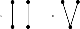
Note that there are families for which . Consider, e.g., the two graphs and depicted in Figure 3.1.
It is easy to see that
and , while for all .
For families of -graphs not containing any -partite hypergraphs, there is the following simple but strong lower bound:
Lemma 3.2.3.
If a family of -graphs has no -partite member, there is a such that for large enough .
Proof.
Consider the complete -partite -graph with which has vertices. It is called the complete equipartite -graph on vertices. This -graph is -free because all of its subgraphs are -partite. It has edges for some . ∎
As a -graph on vertices can have at most as many edges as the complete -graph, we have a trivial upper bound of . Note that the lower bound for non--partite -graphs above is of the same order.
For complete -partite -graphs with partition sets of fixed size, Erdős [Erd64] proved the following upper bound which we will later use:
Theorem 3.2.4 (Erdős [Erd64, Theorem 1]).
Let . Then there is such that for all .
A survey on extremal hypergraph theory is [Für91], where this result can be found (without proof) in Chapter .
3.3 An Upper Bound for the Case
We now use the above concepts to achieve an upper bound on the size of a simplicial complex not containing as subcomplexes any of the non-embeddable complexes we introduced in Section 1.2, which is then also an upper bound for Problem 1.3.2. Recall Theorem 1.2.9:
Theorem 1.2.9 (Schild [Sch93, Theorem 3.1]).
Let be simplicial complexes and suppose there are such that is nice on . Then is not embeddable in for .
Except for the following two cases the complex is minimal non-embeddable, i.e., every proper subcomplex is linearly embeddable in :
- 1.
All are simplices.
- 2.
is the boundary of a simplex with an additional vertex ().
Remember that a simplicial complex on at most vertices, with a vertex set identified with some is called nice on if the following condition holds:
We will consider the -graphs corresponding to the complexes that appear in Theorem 1.2.9. The last section showed that the -partite ones among them are of particular interest. For the case , where is the dimension of , we can show that these complexes have a certain form. This enables us to characterize those among them that correspond to -partite -graphs. For it seems harder to find such a characterization. This is why, from now on, we will only consider the case .
With the notation introduced in the last section we are thus interested in where is the following family of hypergraphs:
Definition 3.3.1 ().
Let . Denote by the family of hypergraphs induced by -dimensional joins of nice complexes that by Theorem 1.2.9 do not embed in :
Let us now try to find a different description of . First, we observe that the dimension of a nice complex is bounded:
Lemma 3.3.2.
If a simplicial complex with is nice on , we have .
Proof.
Let be a simplicial complex with that is nice on .
A -dimensional complex does not contain any simplex with . This means that has to contain all simplices with . Hence, and therefore . Furthermore, cannot contain because . Thus, . ∎
With this lemma we can now determine the structure of those joins of nice complexes for which where is the dimension of the join:
Lemma 3.3.3.
For let be a complex that is nice on . Set
where , and suppose that
Then for , and therefore
Proof.
This determines : Let with . Then cannot be an element of because . Since is nice, it hence has to contain all such . Therefore, . ∎
This also shows that all complexes in are minimal non-embeddable, since none of the two exceptional cases in Theorem 1.2.9 applies.
For this shows that in there are only three complexes: , and . We already used this in Section 2.4 where we showed that none of these three appears as a subcomplex when a missing face is added to the boundary of .
For , the case of planar graphs, this yields that consists exactly of the two graphs and that characterize the planarity of graphs.
By Lemma 3.2.3 only the -partite -graphs in can yield interesting upper bounds. The following lemma characterizes these:
Lemma 3.3.4.
For let and . Furthermore, set .
Then corresponds to a -partite hypergraph if and only if for all .
Proof.
Suppose that at least one of the is not -dimensional. We can assume w.l.o.g. that there is such that for and for .
To show -partiteness we would have to partition the vertices of into subsets such that for any two vertices in a common subset there is no simplex containing both vertices. For such a partition we have:
- •
Any two vertices in different constitute a simplex of the join and hence have to be contained in different :
- •
For the complex has a complete -skeleton, therefore its vertices each need to be contained in different :
Thus, the number of parts of the partition would at least have to be
This shows that, if such a exists, cannot be -partite. Hence, all of the have to be -dimensional for to be -partite.
Now assume that for all . Then , the -fold join of the complex consisting of only three vertices. This complex has dimension . Because no simplex of can contain two vertices from the same copy of , its vertex set can be partitioned into subsets each containing the three vertices of one . ∎
Thus, there is only one hypergraph we can exclude in search for an upper bound: the one corresponding to . We just proved that this hypergraph is -partite, where the partition of the vertex set consists of sets of size . Given this partition, every set containing exactly one vertex from each partition set is an edge. This shows that this hypergraph is the complete -partite -graph . (See Figure 3.2.)

Proposition 3.3.5.
Let and . Then
Proof.
This bound slightly improves the trivial upper bound of , but does not get near the conjectured bound in Conjecture 1.4.4 and the lower bound of that we achieved in Chapter 2.
Our estimate for is hence not very precise. In the case we now have:
for large enough .
Observe that for graphs () we get an upper bound of the order . One might think that is linear in . But remember that we are only excluding and as subgraphs, not as subdivisions or minors! Actually, we will see in the upcoming sections that .
3.4 Improving the Upper Bound?
In the previous section, we bounded the number of maximal simplices in a -complex that embeds into by giving an upper bound for . We now want to study how much could be gained by estimating more precisely.
To achieve this, we will, by means of the probabilistic method, prove a lower bound for for any finite family of -graphs in which each member has at least edges. This will show that for each and for large enough , there has to be an -free -graph with vertices and at least edges for some . We first introduce the concept of random hypergraphs and state a few basic results which we will need for the proof.
3.4.1 Random Hypergraphs
Introductions to random (2-)graphs can be found in [AS00, Chapter 10] and [MU05, Chapter 5]. A concept for random hypergraphs is mentioned in [JŁR00]. We assume knowledge of basic probability theory.
We first describe the Erdős-Rényi model for random hypergraphs, as this is the model that we will be using. The idea is to build a random -graph on the vertex set edge by edge, including each edge with probability . Formally, this works as follows:
Definition 3.4.1 ().
Let , and .
For a set , we consider the Bernoulli trial with sample space
and measure where
Running this trial independently for every set yields the probability space (, which we denote by .
Its sample space can be identified with the set of all possible -graphs on the vertex set . The underlying measure is
We will write to denote that we consider the -graph as an elementary event in .
The number of “successes” in this series of Bernoulli trials is the number of edges of the resulting hypergraph. We thus get:
Lemma 3.4.2.
Let and . Let denote the number of edges of . Then is a binomially distributed random variable with parameters and and hence .
We will also need an estimate for the expected number of subgraphs of a random -graph that are isomorphic to a certain fixed hypergraph.
Lemma 3.4.3.
Let , and a -graph with vertices and edges. Let denote the number of subgraphs of that are isomorphic to .
Then where .
Proof.
For let be the indicator function of , i.e., for we have
Then
With this notation we can express as the sum over for all that are isomorphic to . We thus get:
where the sums range over all that are isomorphic to . The number of such is where is the number of subsets of that are isomorphic to . Thus for we have
∎
We will furthermore need two well known inequalities, Markov’s inequality and Chernoff’s inequality, to estimate the probability of events describing the difference of a random value and its expected value.
Theorem 3.4.4 (Markov’s inequality, e.g., [MU05, Theorem 3.1]).
Let be a random variable with only non-negative values and let . Then
Theorem 3.4.5 (Chernoff’s inequality, e.g., [MU05, Corollary 4.6]).
Let be a binomially distributed random variable and . Then
The following lemma, with which we conclude this section, is a statement on general probability spaces, the generalization of the simple rule
Lemma 3.4.6.
Let be a probability space and events with for all . Then the intersection of the has positive probability: .
Proof.
For an event let denote the complementary event . We have and therefore Hence,
∎
3.4.2 A Lower Bound on
Let be a finite family of -graphs in which each member has at least edges. We will now use the probabilistic tools we just introduced to prove a lower bound for for large enough . We will show that if every hypergraph in has less than vertices and more than edges, there is a such that for large there has to be an -free -graph with vertices and at least edges.
At the end of this section we will then apply this to the family , achieving
for some and for large enough .
The idea for the proof of the general lower bound is similar to the one for proving the existence of graphs with large girth and large chromatic number (e.g., [AS00, p. 38]): We will show that there is a hypergraph which only contains “few” of the forbidden subgraphs in while having “a lot” of edges, by proving that the probability of the event “ has many edges and only few forbidden subgraphs” is greater than zero. We can choose the numbers of edges and subgraphs such that we can then delete one edge from every forbidden subgraph in and still keep sufficiently many edges.
Proposition 3.4.7 ([Sch08]).
For let be a finite family of -uniform hypergraphs and , with such that
Then there is and such that for every there exists an -free -graph on vertices that has at least edges, i.e.,
Proof.
Let for some such that for all . For and let denote the number of subgraphs of that are isomorphic to ; shall denote the number of edges of .
We want to show that we can choose and such that a suitable event of the form “ is large and is small for all ” has positive probability. Lemma 3.4.6 shows that such an intersection of events has probability greater than zero if each of the events occurs with a certain probability. Markov’s Inequality (Theorem 3.4.4) and Chernoff’s Inequality (Theorem 3.4.5) are the tools we will use to estimate the probabilities of the single events.
Let . The events we want to consider are for and .
If the intersection of these events occurs, i.e., , then contains at most copies of each and has at least edges.
Do these events have large enough probability? For , Markov’s Inequality shows that
To estimate the probability of the event we first consider its complementary event. Because is a binomially distributed random variable with parameters and (Lemma 3.4.2), Chernoff’s Inequality yields
Hence, if and is large enough, we get
Lemma 3.4.6 now tells us that
Thus, for and large enough there is a -graph on vertices that contains at most copies of each and has at least edges.
Now, we want to choose and such that after removing one edge from every forbidden subgraph sufficiently many edges remain. The number of edges we have to remove is at most . So, if we want to keep at least half of the edges we have to have
| (3.1) |
How large is ? Lemma 3.4.3 tells us that for there exists such that
Therefore, setting , we have
What about the other side of (3.1)? With we get
Hence, (3.1) is fulfilled if , which is equivalent to
Because ,
This means, we want to find values for and such that
| (3.2) |
If we choose
we have and the left side of (3.2) is . Thus, (3.2), and therefore also (3.1), is fulfilled.
Is this an admissible choice of these parameters? Two things have to be considered: We need and, to guarantee that is large enough, .
If we choose we have . Since
we also get that . The last condition is also fulfilled because by assumption which is equivalent to
Thus, for and suitable after removing at most half of the edges of we get an -free graph that has at least edges for . ∎
Remark 3.4.8.
Proving for some is a little bit easier. One can simply set and, by proceeding as above, get to which is fulfilled for and large enough .
To apply this result to the family , we need to know an upper bound for the number of vertices and a lower bound for the number of edges of the hypergraphs in . The following lemma shows that the hypergraph , which corresponds to the complex , determines both of these bounds.
Lemma 3.4.9.
Let . Among all -complexes corresponding to hypergraphs in the complex has the maximal number of vertices and the minimal number of -simplices.
Proof.
Let be a simplicial complex that corresponds to an element of . By Lemma 3.3.3 there are and with such that where .
We have . Hence, the number of vertices of is maximal if is maximal. But . So, is maximal if for all . The number of -simplices of is . The sequence is strictly increasing because
Hence, each of the factors is minimal for . ∎
With this we get the desired lower bound for :
Proof.
To conclude the part on upper bounds let us summarize our results. For all and for large we now have:
which shows that improving the upper bound on, or even determining could not close the gap between the upper bound of and the lower bound of for by much. For we get
for large enough . Observe that for the case we proved the existence of a graph containing neither nor with at least edges for large . However, simple explicit constructions for such graphs are already known. One example is the following: Since both and contain a quadrilateral , quadrilateral-free graphs are examples of - and -free graphs. It is known that for any prime power there is a graph with vertices and edges, defined by the points and lines of the projective plane over the field , that doesn’t contain a quadrilateral ([ERS66], [Bro66]).
Further Thoughts
We could achieve a lower bound of for all such that in Chapter 2. For we could also prove that this bound can not be improved by simply adding simplices.
In Chapter 3 we could improve the trivial upper bound of by giving an upper bound of
We could also see that a better estimate of would not improve this bound considerably by showing that
To conclude, we now collect some ideas that could be pursued to get better results for Problem 1.3.2. To get Corollary 3.4.10 we proved the existence of an -free -graph on vertices with at least
edges for large . For the case this shows that for large there is a graph not containing and with at least edges. By Wagner’s Theorem (Theorem 1.2.7) these two graphs characterize planar graphs as excluded minors; Kuratowski’s Theorem (Theorem 1.2.6) states that excluding subdivisions of and gives all planar graphs. As the maximum size of a planar graph is of linear order (Lemma 1.3.5), this shows that in this case the order of the maximal number of edges changes if one excludes subdivisions or minors instead of subgraphs.
This gives rise to hopes that excluding subdivisions of the hypergraphs in or excluding themselves as minors might lead to a better upper bound than the one achieved in Proposition 3.3.5. However, while the concepts of subdivisions and minors are well understood for graphs, they appear to be not as clear and are less studied in the context of hypergraphs. In addition to that, the connection to embeddability is not as obvious. Nevo’s concept of minors for simplicial complexes, which was used in this thesis, (Definition 2.4.5) doesn’t seem to translate easily to hypergraphs.
Another idea which doesn’t seem easy to rule out is to use the Upper Bound Theorem for spheres in the following way: If a -complex on vertices is a subcomplex of some simplicial -sphere with vertices, we know that by the Upper Bound Theorem for spheres. Suppose we would know that every -complex on vertices that embeds into is a subcomplex of such a sphere. This seems unlikely, but there also seems to be no counterexample yet. If it were true, we would have an upper bound of for Problem 1.3.2, which would at least be of the same order as the one in Conjecture 1.4.4.
Furthermore, it might be possible to show that it suffices to prove Conjecture 1.4.4 for all even . The approach to this draws on the idea of the proof of Lemma 1.3.7, the solution for the case and , which depends on the solution for the case and (planar graphs).
In this proof, the lower dimensional case gives upper bounds for the -vectors of the vertex links of the complex. These bounds are then, via double counting, used to determine an upper bound for the whole complex. An adaptation of this proof for higher odd dimensions seems possible. For odd , we have , while . Thus, the additional factor of , which arises by summing over all vertices, conserves the right order in the odd case, whereas this inductive idea clearly fails for even . This idea might also work for reasonable upper bounds in even dimensions, other than .
References
- [AS00] Noga Alon and Joel Spencer, The Probabilistic Method, second ed., Wiley-Interscience Series in Discrete Mathematics and Optimization, John Wiley & Sons Inc., 2000.
- [BGdO00] Jürgen Bokowski and António Guedes de Oliveira, On the generation of oriented matroids, Discrete Comput. Geom. 24 (2000), no. 2-3, 197–208.
- [BK88] Anders Björner and Gil Kalai, An extended Euler-Poincaré theorem, Acta Math. 161 (1988), no. 1, 279–303.
- [Bol02] Béla Bollobás, Modern Graph Theory, Graduate Texts in Mathematics, Springer-Verlag, 2002.
- [Bre83] Ulrich Brehm, A nonpolyhedral triangulated Möbius strip, Proc. Amer. Math. Soc. 89 (1983), no. 3, 519–522.
- [Bro66] William G. Brown, On graphs that do not contain a Thomsen graph, Canad. Math. Bull. 9 (1966), no. 3, 281–285.
- [Bry72] John L. Bryant, Approximating embeddings of polyhedra in codimension three, Trans. Amer. Math. Soc. 170 (1972), 85–95.
- [BS92] Ulrich Brehm and Karanbir S. Sarkaria, Linear vs. piecewise linear embeddability of simplicial complexes, Tech. Report 92/52, Max-Planck-Institut f. Mathematik, Bonn, Germany, 1992.
- [DE94] Tamal K. Dey and Herbert Edelsbrunner, Counting triangle crossings and halving planes, Discrete Comput. Geom. 12 (1994), 281–289.
- [DP98] Tamal K. Dey and János Pach, Extremal problems for geometric hypergraphs, Discrete Comput. Geom. 19 (1998), 473–484.
- [Erd64] Paul Erdős, On extremal problems of graphs and generalised graphs, Israel J. Math. 2 (1964), no. 3, 183–190.
- [ERS66] Paul Erdős, Alfréd Rényi, and Vera T. Sós, On a problem of graph theory, Studia Sci. Math. Hungar. 1 (1966), 215–235.
- [Flo33] A. Flores, Über -dimensionale Komplexe, die nicht in den topologisch einbettbar sind, Ergebnisse eines mathematischen Kolloquiums 5 (1932/1933), 17–24.
- [Flo34] , Über -dimensionale Komplexe, die im absolut selbstverschlungen sind, Ergebnisse eines mathematischen Kolloquiums 6 (1933/1934), 4–7.
- [Für91] Zoltán Füredi, Turán type problems, Surveys in Combinatorics, 1991 (A. D. Keedwell, ed.), London Mathematical Society Lecture Note Series, vol. 166, Cambridge Univ. Press, 1991.
- [Grü69] Branko Grünbaum, Imbeddings of simplicial complexes, Comment. Math. Helv. 44 (1969), 502–513.
- [Grü03] , Convex Polytopes : Second Edition Prepared by Volker Kaibel, Victor Klee, and Günter Ziegler (Graduate Texts in Mathematics), Springer-Verlag, New York, 2003.
- [HJ64] Rudolf Halin and Heinz A. Jung, Charakterisierung der Komplexe der Ebene und der -Sphäre, Arch. Math. 15 (1964), 466–469.
- [JŁR00] Svante Janson, Tomasz Łuczak, and Andrzej Ruciński, Random Graphs, Wiley-Interscience Series in Discrete Mathematics and Optimization, John Wiley & Sons Inc., 2000.
- [Kal84] Gil Kalai, Characterization of -vectors of families of convex sets in , Part I: Necessity of Eckhoff’s conditions, Israel J. Math. 48 (1984), no. 2, 175–195.
- [Kal85] , -Vectors of acyclic complexes, Discrete Math. 55 (1985), no. 1, 97–99.
- [Kal88] , Many triangulated spheres, Discrete Comput. Geom. 3 (1988), no. 1, 1–14.
- [Kal91] , The diameter of graphs of convex polytopes and -vector theory, Applied Geometry and Discrete Mathematics, The Victor Klee Festschrift (Peter Gritzmann and Bernd Sturmfels, eds.), DIMACS Series in Discrete Mathematics and Theoretical Computer Science, vol. 4, 1991, pp. 387–411.
- [Kal02] , Algebraic shifting, Computational Commutative Algebra and Combinatorics, Advanced Studies in Pure Mathematics, vol. 33, Mathematical Society of Japan, 2002, pp. 121–163.
- [Kal08] , Extermal [sic] combinatorics ii: Some geometry and number theory, Combinatorics and more - Gil Kalai’s blog, July 2008, http://gilkalai.wordpress.com/2008/07/17/extermal-combinatorics-ii-some-geometry-and-number-theory/.
- [Lic99] W. B. Raymond Lickorish, Simplicial moves on complexes and manifolds, Geometry and Topology Monographs 2 (1999), 299–320.
- [Mat03] Jiří Matoušek, Using the Borsuk–Ulam theorem: Lectures on Topological Methods in Combinatorics and Geometry, Universitext, Springer-Verlag, Berlin, 2003.
- [McM70] Peter McMullen, The maximum numbers of faces of a convex polytope, Mathematika 17 (1970), 179–184.
- [MTW09] Jiří Matoušek, Martin Tancer, and Uli Wagner, Hardness of embedding simplicial complexes in , SODA ’09: Proceedings of the Nineteenth Annual ACM -SIAM Symposium on Discrete Algorithms, Society for Industrial and Applied Mathematics, 2009, pp. 855–864.
- [MU05] Michael Mitzenmacher and Eli Upfal, Probability and Computing: Randomized Algorithms and Probabilistic Analysis, Cambridge University Press, 2005.
- [Mun93] James R. Munkres, Elements of Algebraic Topology, Perseus Books, New York, 1993.
- [Mur07] Satoshi Murai, Algebraic shifting of cyclic polytopes and stacked polytopes, Discr. Mathematics 307 (2007), no. 14, 1707–1721.
- [Nev07] Eran Nevo, Higher minors and Van Kampen’s obstruction, Math. Scand. 101 (2007), 161–176.
- [Nov03] Isabella Novik, Remarks on the upper bound theorem, Combin. Theory Ser. A 104 (2003), no. 1, 201–206.
- [NW08] Eran Nevo and Uli Wagner, On the embeddability of skeleta of spheres, 2008, to appear in Israel J. Math.
- [Sar91] Karanbir S. Sarkaria, Kuratowski complexes, Topology 30 (1991), no. 1, 67–76.
- [Sch93] Göran Schild, Some minimal nonembeddable complexes, Topology Appl. 53 (1993), 177–185.
- [Sch06] Lars Schewe, Generation of oriented matroids using satisfiability solvers, Mathematical Software - ICMS 2006, Lecture Notes in Computer Science, vol. 4151/2006, Springer Berlin/Heidelberg, 2006, pp. 216–218.
- [Sch08] Mathias Schacht, Personal communication, February 2008.
- [Sta75] Richard P. Stanley, The Upper Bound Conjecture and Cohen-Macaulay rings, Stud. Appl. Math. 54 (1975), 135–142.
- [Sta96] , Combinatorics and Commutative Algebra, second ed., Progress in Mathematics, vol. 41, Birkhäuser, 1996.
- [Umm73] Brian R. Ummel, Imbedding classes and -minimal complexes, Proc. Amer. Math. Soc. 38 (1973), 201–206.
- [vK32a] Egbert Rudolf van Kampen, Berichtigung zu Komplexe in euklidischen Räumen, Abh. Math. Sem. Hamburg 9 (1932), 152–153.
- [vK32b] , Komplexe in euklidischen Räumen, Abh. Math. Sem. Hamburg 9 (1932), 72–78.
- [Wes01] Douglas B. West, Introduction to Graph Theory, second ed., Prentice Hall, 2001.
- [Zak69a] Joseph Zaks, On a minimality property of complexes, Proc. Amer. Math. Soc. 20 (1969), no. 2, 439–444.
- [Zak69b] , On minimal complexes, Pacif. J. Math. 28 (1969), no. 3, 721–727.
- [Zie98] Günter M. Ziegler, Lectures on Polytopes, second ed., Graduate Texts in Mathematics, Springer-Verlag, 1998.
Zusammenfassung
Es ist nicht schwer zu zeigen, dass jeder -dimensionale Simplizialkomplex eine Einbettung in den besitzt. Demzufolge ist die maximale Anzahl von -Simplizes für einen in diesen Raum einbettbaren Komplex, der Ecken besitzt, .
Für dem Fall liefert dies für Einbettbarkeit in den . Mit elementaren Methoden kann auch gezeigt werden, dass ein -dimensionaler Simplizialkomplex auf Ecken, der in den eingebettet werden kann, höchstens aus Dreiecken besteht. Für in den eingebettete -Komplexe ist die Frage der maximalen Anzahl an Dreiecken ungeklärt.
Diese Arbeit befasst sich mit der allgemeineren Frage, wieviele maximale Simplizes ein -dimensionaler Simplizialkomplex, der sich in den , für , einbetten lässt, höchstens enthalten kann. Mit Hilfe von zyklischen Polytopen, deren Randkomplexe Beispiele einbettbarer Komplexe bilden, erhält man die untere Schranke .
Es wird gezeigt, dass das Hinzufügen eines weiteren Simplizes zu dem Komplex bei Verwendung der vorhandenen Ecken zu einem nicht mehr in den einbettbaren Komplex führt. Die Schranke kann also nicht auf diesem einfachen Wege verbessert werden.
Um eine obere Schranke zu bekommen, wird hier die Idee auszuschließender Unterkomplexe verfolgt. Eine Verallgemeinerung des Satzes von van Kampen und Flores liefert eine Klasse von nicht in den einbettbarer Komplexen. Ein Simplizialkomplex, der einen solchen als Unterkomplex besitzt, kann ebenfalls nicht einbettbar sein. Demzufolge enthält die Klasse der Komplexe, die kein Oberkomplex eines dieser nicht einbettbaren Komplexe sind, die Klasse der in den einbettbaren Komplexe.
Für den Fall kann mit den Methoden der extremalen Hypergraphentheorie eine obere Schranke für die maximale Anzahl von Simplizes in einem Simplizialkomplex, in dem die gegebenen nicht einbettbaren Komplexe als Unterkomplexe verboten sind, gefunden werden. Diese ist also auch eine obere Schranke für die eigentliche Fragestellung im Fall und hat die Größenordnung . Desweiteren wird gezeigt, dass man auf diesem Wege keine bessere Abschätzung als erhalten kann.