subject
Article\Year2018 \MonthDecember \Vol62 \No1 \DOI10.1007/s11432-016-0037-0 \ArtNo000000 \ReceiveDateNovember 20, 2018 \AcceptDateDecember 6, 2018
Condensation of Eigen Microstate in Statistical Ensemble and Phase Transition
chenxs@bnu.edu.cn
Hu G K
Hu G K, Liu T, Liu M X, et al
05.50.+q, 05.70.Fh
Condensation of Eigen Microstate in Statistical Ensemble and Phase Transition
Abstract
In a statistical ensemble with microstates, we introduce an correlation matrix with the correlations between microstates as its elements. Using eigenvectors of the correlation matrix, we can define eigen microstates of the ensemble. The normalized eigenvalue by represents the weight factor in the ensemble of the corresponding eigen microstate. In the limit , weight factors go to zero in the ensemble without localization of microstate. The finite limit of weight factor when indicates a condensation of the corresponding eigen microstate. This indicates a phase transition with new phase characterized by the condensed eigen microstate. We propose a finite-size scaling relation of weight factors near critical point, which can be used to identify the phase transition and its universality class of general complex systems. The condensation of eigen microstate and the finite-size scaling relation of weight factors have been confirmed by the Monte Carlo data of one-dimensional and two-dimensional Ising models.
1 Introduction
In statistical physics, the concept of ensemble in phase space serves as a starting point. An ensemble in phase space is composed of the microstates of system under some thermodynamic conditions. Thermodynamic quantities of system can be obtained by the ensemble-average with the summation over all microstates of the ensemble.
Three important thermodynamic ensembles were defined by J. W. Gibbs [1]. They are the micro-canonical ensemble, the canonical ensemble, and the grand canonical ensemble. The micro-canonical ensemble is under the\Authorfootnote
thermodynamic conditions that the number of particles , the volume , and the total energy of system are fixed. In the canonical ensemble, the energy of system is not known exactly. In place of the energy, the temperature is specified. In the grand canonical ensemble, neither the energy nor particle number are fixed. In their place, the temperature and chemical potential are specified.
In computer simulations or experimental investigations of complex systems under some conditions, snapshots of system can be taken. From these snapshots, we can obtain at first microstates and then a statistical ensemble of the system. In this paper, we study the correlations between microstates in the statistical ensemble. With the correlations between microstates as its elements, we can get a correlation matrix of microstate in the statistical ensemble. Using the eigenvectors of the correlation matrix, the eigen microstates of the statistical ensemble can be defined. The normalized eigenvalues by the number of microstate represent the weight factors of the corresponding eigen microstates in the ensemble. The distribution of eigen microstate in the statistical ensemble can be described by all weight factors.
Our paper is organized as follows. In Section 2, we introduce the correlation between microstate and a correlation matrix. Using its eigenvectors, the eigen microstates of the ensemble are calculated. In one-dimensional and two-dimensional Ising models, their eigen microstates and eigenvalues are studied using the Monte Carlo (MC) simulations. In Section 3, we propose a finite-size scaling relation of the weight factors near critical point, which is confirmed by MC simulation data of Ising models. We make some conclusions finally in Section 4.
2 Eigen microstates of statistical ensemble and condensation
We consider an Ising model with the Hamiltonian
| (1) |
where is the spin on site and is the interaction between spins and . For the Ising model with spins, a microstate of system can be described by a vector with components as
which is normalized and . The total energy of system at microstate can be written as with the interaction matrix defined by .
At temperature , the microstate has a probability
| (7) |
where and is the Boltzmann constant. In MC simulations, different microstates of system can be sampled with the probability factor. microstates from simulation are taken to build up an ensemble. The correlation between microstates and is defined as
| (8) |
If , . When , . We have in general.
With as its elements, an correlation matrix is obtained. We suppose that has eigenvectors with associated eigenvalues . We arrange all eigenvalues in the order . There is a relation
| (9) |
where
The normalized eigenvectors are orthogonal each other and follow the relation
| (15) |
where is the Kronecker delta. The trace of the correlation matrix is .
From the eigenvectors, we can define an matrix
| (16) |
with elements . is an orthogonal matrix and satisfies the condition . After the transformation of the correlation matrix, we have , where is a diagonal matrix with elements .
Using the components of an eigenvector , we can introduce an eigen microstate
| (17) |
which satisfies the relation . The correlation between eigen microstates and is
| (18) |
Therefore, the correlation matrix is diagonal and there is no correlation between eigen microstates.
In the ensemble consisting of original microstates, all microstates have the same weight. The weight factor of microstate
| (19) |
which satisfies the normalization condition .
In the ensemble consisting of eigen microstates, different microstates have different weights. We define the weight factor of eigen microstate as
| (20) |
which satisfies a normalization condition .
In an ensemble without localization of microstate, all weight factors in the limit . If the largest weight factor becomes finite in the limit , this indicates a condensation of eigen microstate in the ensemble. This condensation of microstate is similar to the Bose-Einstein condensation [2]. Now system has a phase transition with the new phase characterized by the eigen microstate .
The eigenvalue depends on , , and and . In the limit at fixed , an eigenvalue function is obtained. The normalized condition of eigenvalue function is
| (21) |
In the limit , the finite implies that the eigenvalue function when .
Original microstates can be expressed by eigen microstates as
| (22) |
Since , a normalized eigen microstate is introduced. With normalized eigen microstates, We have
| (23) |
In the ensemble of original microstate, the magnetization of system can be calculated as
| (24) |
where
| (25) |
is the magnetization of original microstate .
Equivalently, we can write the magnetization of system according to Eq. (22) as
| (26) |
where
| (27) | |||||
| (28) |
Other thermodynamics quantities of system can be calculated in a similar way.
In the following, we will study the eigen microstates and their weight factors in the statistical ensembles of one-domensional and two-dimensional Ising models.
2.1 One-dimensional Ising model
The one-dimensional (1d) Ising model with the nearest-neighbour interaction has the Hamiltonian
| (29) |
Under the periodic boundary condition , this model can be solved exactly [3]. In the thermodynamic limit , its correlation function has an exponential form
| (30) |
with the correlation length
| (31) |
where is the lattice spacing and . In a finite 1d-Ising chain with periodic boundary condition, the system has susceptibility [4]
| (32) |
where . The correlation length when . Although it has been well acknowledged that there is no phase transition in such an 1d-Ising model, we can still consider the zero temperature as a critical point since the correlation length diverges. The thermodynamic quantities of 1d-Ising model should have similar critical behaviors above as that of -dimensional Ising model with . Near , the susceptibility satisfies asymptotically a finite-size scaling relation
| (33) |
with [3] and the finite-size scaling function
| (34) |
Using the hyperscaling relation for 1d-Ising model, we obtain , which is in agreement with that of Ref. [3].
We simulate the microstates of 1d-Ising model using the Wolff algorithm [5]. Simulations are started with all spins aligned. To get the microstates in equilibrium, the first microstates are not used. The subsequent microstates are chosen at an interval of 205 MC steps to keep their independence. Using the microstates obtained, we can get the correlation matrix . With the eigenvectors and eigenvalues of , we can obtain eigen microstates according to Eq. (17).
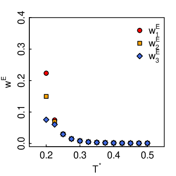
The -dependence of eigenvalue has been studied. At , the -dependence of the largest three normalized eigenvalues can be neglected. We show the largest three normalized eigenvalues at in Fig. 1.
We can see from Fig. 1 that the weight factor become finite with the decrease of temperature. This indicates that there will be a phase transition. To identify the new phase of system, the corresponding eigen microstates should be studied.

At , the eigen microstates of the largest three eigevalues are shown in Fig. 2. In these eigen microstates, spin clusters are of micro scales and distributed with alternate orientation in the real space.

The largest three eigen microstates at are presented in Fig. 3. The sizes of clusters are comparable to that of system. Only one cluster exists in the largest eigen microstate. The second largest eigen microstate has two clusters with opposite orientation. In the third largest eigen microstate, there are four clusters with alternate orientations.
For an overview of the weight distribution of eigen microstate, we define the cumulant
| (35) |

In Fig. 4, the weight cumulants of 1d-Ising model are plotted. At , the cumulant reaches nearly at . So the original microstates are constituted actually by about eigen microstates. At , becomes nearly at , which is still much less than .
2.2 Two-dimensional Ising model
In a two-dimensional (2d) Ising model with linear length and periodic boundary conditions, there are spins in this system. With the nearest neighbor interaction and square lattice, this model has a ferromagnetic phase transition at the reduced temperature [6].
The microstates of the 2d-Ising model are simulated using the Wolff algorithm [5] also. In our simulations, we start with all spins aligned. The first microstates are used to reach the equilibrium. From the subsequent microstates, microstates at each temperature are taken at an interval of 250 MC steps. From the microstates, we can calculate the correlation matrix at first and then its eigenvalues and eigenvectors. The eigen microstates are obtained using the eigenvectors.
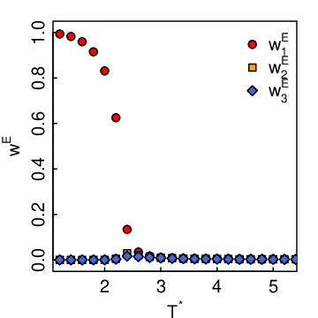
The largest three eigenvalues around the critical point are presented in Fig. 5. The normalized eigenvalue by is equivalent to the weight factor. At temperatures above , the largest three weight factors are quite small. There is no localization of eigen microstate. The weights of eigen microstates are distributed widely. At temperatures below , the largest eigenvalues become finite. This indicates a condensation of the eigen microstate . There is now a phase transition, whose nature is characterized by the condensed eigen microstate.
The largest three eigen microstates at are shown in Fig. 6. The sizes of the spin clusters in the eigen microstates are much smaller than system size.


In Fig. 7, the eigen microstates of the largest three eigenvalues at are presented. There is only one cluster in the eigen microstate of the largest eigenvalue.
We plot in Fig. 8 the eigen microstates of the largest three eigenvalues at . In the largest eigen microstate, there is only one spin cluster. The large- limit of its weight factor is larger than , as shown in Fig. 10. There is a ferromagnetic phase transition. The second largest eigen microstate has two clusters with opposite orientation. There are four spin clusters in the third largest eigen microstate.

With the further decrease of temperature, the largest eigen microstate with one spin cluster becomes more dominant. The weight factor of the largest eigen microstate at is larger than , which can be seen in Fig. 10. Other eigen microstates have many small clusters, as shown in Fig. 9.
The weight cumulants of eigen microstate at are shown in Fig. 10. The weight cumulants reach nearly at . The original microstates are composed of eigen microstates approximately.
3 Finite-size scaling of weight factor near critical point
In the region near a critical point, thermodynamic functions of finite system are proposed to satisfy finite-size scaling relations [7, 8, 9]. For the order parameter, its finite-size relation is
| (36) |
where is the reduced temperature, is the critical exponent of order parameter, and is the critical exponent of bulk correlation length . The scaling variable is related to the size ratio .
The correlation length follows the finite-size scaling form [8]. Recently, a finite-size scaling relation of correlation function was proposed [10]. Using this finite-size relation, the finite-size scaling form of correlation length can be naturally derived. For the principal fluctuation modes of complex system, there is also a finite-size scaling relation [11], which has been confirmed in 2d-Ising model.
Basing on the relation between the weight factor of eigen microstate and the order parameter, we propose a finite-size scaling form
| (37) |
In one-dimensional Ising model, the critical exponent and , where is given in Eq. (31). We present the largest two weight factors with respect to and scaling variable in Fig. 11. The finite-size scaling form of Eq. (37) is confirmed in 1d-Ising model.

In two-dimensional Ising model, the critical exponents and [6]. On the left side of Fig. 12, the largest weight factor of are plotted with respect to . The finite-scaling form is presented with respect to on the right side. The different curves for different collapse together. The finite-size relation of Eq. (37) is confirmed in 2d-Ising model.


In Figs. 13 and 14, the second and third largest weight factors and their finite-size scaling form are presented.
After taking logarithm of Eq. (37), we obtain
| (38) |
which depends on linearly at . This property can be used to determine the critical point and the critical exponent ratio .

In Fig. 15, the log-log plot of the largest weight factor with respect to is presented at different reduced temperatures. The curves are curved upward at and downward at . From the straight line at , we can obtain , which is in agreement with the exact value [6].
We introduce the ratio of weight factor , which follows the finite-size scaling form
| (39) |
At the critical point, the ratio is independent of . This can be used to determine the critical point also.

The ratio of 2d-Ising model is plotted in Fig. 16. With as the variable, curves of different have a fixed point at . Using as the variable, the curves collapse together.
Therefore, the finite-size scaling relation of weight factor in Eq. (37) has been verified in one-dimensional and two-dimensional Ising models. We anticipate that this finite-size relation is valid for general complex systems.
4 Conclusions
In the phase space of a complex system, we introduce the eigen microstates of its statistical ensemble. The microstates of the complex system under some conditions can be obtained from computer simulations or experimental studies. We introduce a correlation matrix with correlations between microstates as its elements. Using the eigenvectors of the correlation matrix, the eigen microstates of the ensemble can be defined. The normalized eigenvalues by the number of microstate can be considered as the weight factor in the ensemble of the corresponding eigen microstates.
In an ensemble without localization of microstate, weight factors of eigen microstate go to zero when . If the largest weight factor becomes finite in the limit , there is a condensation of the eigen microstate in the ensemble. This condensation indicates a phase transition with the new phase characterized by the eigen microstate corresponding to the finite weight factor. We propose a finite-size scaling relation of the weight factors near critical point using the critical exponents of order parameter and correlation length.
The eigen microstates and their weight factors in an ensemble of one-dimensional and two-dimensional Ising models have been studied using Monte Carlo simulation. The condensation of eigen microstate in the one-dimensional Ising model appears when . All spins of the condensed eigen microstate have the same orientation and there is a ferromagnetic phase transition. In two-dimensional Ising model, condensations of eigen microstate are found at the reduced temperatures . In the condensed eigen microstate, all spins have the same orientation and there is a ferromagnetic phase transition in two-dimensional Ising model. The finite-size scaling relation of weight factors is confirmed by the Monte Carlo simulation results of one-dimensional and two-dimensional Ising models. Further, we will study the eigen microstates and their weight factors of statistical ensemble for complex systems such as confined fluids [12], networks with long-range connections [13], and climate systems [14].
In the studies of phase transitions of complex systems, the definition of order parameter is sometimes a challenge. We can take collective motion as an example. Collective motion exists at almost every scale in nature, from unicellular organisms to bird flocks, fish schools, and human crowds [15]. The simple model of collective motion was introduced by Vicsek and collaborators [16].The transition to collective motion in the Vicsek model (VM) is thought to be critical [16] and discontinuous [17]. More phases such as ordered ”Toner-Tu” phase [18] and band phases [19, 20, 21] are suggested to exist in the VM. A global understanding and the real order parameter of the transition to collective motion is still lacking. Using the method proposed here, we can determine the critical point, the order parameter, and the critical exponents of complex system at the same time. Our method of analysis is not restricted to systems in equilibrium.
This work was support by Key Research Program of Frontier Sciences, Chinese Academy of Sciences (Grant No. QYZD-SSW-SYS019). Our Monte Carlo simulations are supported by HPC Cluster of ITP-CAS. We are grateful to insight discussions with Prof. Jinghai Li.
The authors declare that they have no conflict of interest.
References
- [1] J. Willard Gibbs. Elementary Principles in Statistical Mechanics. New York: Charles Scribner’s Sons, 1902.
- [2] Lev Petrovich Pitaevskiĭ and S Stringari. Bose-Einstein Condensation. Clarendon Press, 2003.
- [3] Rodney J Baxter. Exactly Solved Models in Statistical Mechanics. Academic Press, London, 1982.
- [4] XiaoSong Chen and Volker Dohm. Relation between bulk order-parameter correlation function and finite-size scaling. The European Physical Journal B - Condensed Matter and Complex Systems, 15(2):283–296, 2000.
- [5] Ulli Wolff. Collective monte carlo updating for spin systems. Phys. Rev. Lett., 62(4):361–364, 1989.
- [6] Lars Onsager. Crystal statistics. i. a two-dimensional model with an order-disorder transition. Phys. Rev., 65(3-4):117–149, Feb 1944.
- [7] Michael E. Fisher and Michael N. Barber. Scaling theory for finite-size effects in the critical region. Phys. Rev. Lett., 28(23):8–11, 1972.
- [8] Vladimir Privman and Michael E. Fisher. Universal critical amplitudes in finite-size scaling. Phys. Rev. B, 30:322–327, Jul 1984.
- [9] Vladimir Privman, Ammon Aharony, and P.C. Hohenberg. Universal critical-point amplitude relations. In Cyril Domb and Joel Louis Lebowitz, editors, Phase Transitions and Critical Phenomena, volume 14, page 1. Academic, New York, 1991.
- [10] Xin Zhang, GaoKe Hu, YongWen Zhang, XiaoTeng Li, and XiaoSong Chen. Finite-size scaling of correlation functions in finite systems. Science China Physics, Mechanics & Astronomy, 61(12):120511, Oct 2018.
- [11] XiaoTeng Li and XiaoSong Chen. Critical behaviors and finite-size scaling of principal fluctuation modes in complex systems. Commun. Theor. Phys., 66(3):355, 2016.
- [12] Wei Dong and XiaoSong Chen. Scaled particle theory for bulk and confined fluids: A review. Science China Physics, Mechanics & Astronomy, 61(7):070501, Jul 2018.
- [13] ZiQing Yang, MaoXin Liu and XiaoSong Chen. Criticality of networks with long-range connections. Science China Physics, Mechanics & Astronomy, 60(2):020521, Feb 2017.
- [14] JingFang Fan, Jun Meng, XiaoSong Chen, Yosef Ashkenazy, and Shlomo Havlin. Network approaches to climate science. Science China Physics, Mechanics & Astronomy, 60(1):010531, Jan 2017.
- [15] Tamás Vicsek and Anna Zafeiris. Collective motion. Physics Reports, 517(3-4):71–140, Aug 2012.
- [16] Tams Vicsek, Andrs Czirk, Eshel Ben-Jacob, Inon Cohen, and Ofer Shochet. Novel type of phase transition in a system of self-driven particles. Phys. Rev. Lett., 75(6):1226–1229, Aug 1995.
- [17] Guillaume Grégoire and Hugues Chaté. Onset of Collective and Cohesive Motion. Phys. Rev. Lett., 92(2):025702, Jan 2004.
- [18] John Toner and Yuhai Tu. Long-range order in a two-dimensional dynamical XY model: How birds fly together. Phys. Rev. Lett., 75(23):4326, Dec 1995.
- [19] Eric Bertin, Michel Droz, and Guillaume Grégoire. Boltzmann and hydrodynamic description for self-propelled particles. Phys. Rev. E, 74(2):022101, Aug 2006.
- [20] Shradha Mishra, Aparna Baskaran, and M. Cristina Marchetti. Fluctuations and pattern formation in self-propelled particles. Phys. Rev. E , 81(6):061916, Jun 2010.
- [21] Thomas Ihle. Kinetic theory of flocking: Derivation of hydrodynamic equations. Phys. Rev. E , 83(3):030901, Mar 2011.