Controlling Dispersive Hydrodynamic Wavebreaking in a Viscous Fluid Conduit
Abstract
The driven, cylindrical, free interface between two miscible, Stokes fluids with high viscosity contrast have been shown to exhibit dispersive hydrodynamics. A hallmark feature of dispersive hydrodynamic media is the dispersive resolution of wavebreaking that results in a dispersive shock wave. In the context of the viscous fluid conduit system, the present work introduces a simple, practical method to precisely control the location, time, and spatial profile of wavebreaking in dispersive hydrodynamic systems with only boundary control. The method is based on tracking the dispersionless characteristics backward from the desired wavebreaking profile to the boundary. In addition to the generation of approximately step-like Riemann and box problems, the method is generalized to other, approximately piecewise-linear dispersive hydrodynamic profiles including the triangle wave and N-wave. A definition of dispersive hydrodynamic wavebreaking is used to obtain quantitative agreement between the predicted location and time of wavebreaking, viscous fluid conduit experiment, and direct numerical simulations for a range of flow conditions. Observed space-time characteristics also agree with triangle and N-wave predictions. The characteristic boundary control method introduced here enables the experimental investigation of a variety of wavebreaking profiles and is expected to be useful in other dispersive hydrodynamic media. As an application of this approach, soliton fission from a large, box-like disturbance is observed both experimentally and numerically, motivating future analytical treatment.
Keywords:
Dispersive shock wavesI Introduction
The interfacial dynamics of a viscous fluid conduit exhibit a wide range of dispersive hydrodynamic behavior observable in other geophysical, superfluidic, optical, and condensed matter media El and Hoefer 2016. A viscous fluid rises buoyantly through a more viscous, stationary fluid and, under appropriate conditions, the interface resembles that of a deformable pipe. The interface’s dynamics can be accurately described by the conduit equation Olson and Christensen 1986; Lowman and Hoefer 2013; Whitehead and Helfrich 1988, a nonlinear dispersive partial differential equation that has been shown to admit a rich zoology of multiscale coherent wave solutions Maiden and Hoefer 2016. Experimentally, solitons Scott et al. 1986; Olson and Christensen 1986; Helfrich and Whitehead 1990, dispersive shock waves (DSWs), and the interactions between them Lowman et al. 2013; Maiden et al. 2016; Maiden et al. 2018 have been observed to be in excellent agreement with conduit equation predictions. In this sense, the viscous fluid conduit is an ideal laboratory environment for the study of dispersive hydrodynamics.
Dispersive shock waves are coherent structures that are fundamental to dispersive hydrodynamics El and Hoefer 2016. A DSW is an expanding, oscillating train of amplitude-ordered nonlinear waves composed of a large amplitude solitary wave adjacent to a monotonically decreasing wave envelope that terminates with a packet of small amplitude dispersive waves. DSWs result when nonlinear self-steepening is compensated by conservative wave dispersion in contrast to the viscous shock waves of dissipative media. The model problem for shock generation is the Riemann problem that consists of an initial, sharp step in amplitude.
A major challenge for the experimental study of DSWs is the controlled realization of wavebreaking that involves the spontaneous generation of oscillations when nonlinear self-steepening enhances small-scale dispersive processes. One obstacle to the laboratory generation of a desired wavebreaking profile is its reliable initiation from only boundary control. Laboratory nonlinear dispersive wave environments constrained by boundary control include fluids such as shallow water wave tanks (see, e.g. Trillo et al. 2016) and viscous fluid conduits Scott et al. 1986. Also included are non-fluid systems such as intense laser light propagation in optical fibers Xu et al. 2017, magnetic spin waves Janantha et al. 2017, and granular crystals Chong et al. 2017. It can be difficult to achieve controlled wavebreaking conditions without boundary interactions. Here, we report on a simple mathematical observation that yields a feasible way to achieve a variety of wavebreaking profiles away from boundaries. We track the (long-wave) characteristics of the dispersionless conduit equation backwards in time from the desired wavebreaking profile. The resulting solution is then used as a boundary condition for conduit experiments to realize a variety of wavebreaking profiles at desired spatial locations. This technique was used to generate dispersive hydrodynamic flows in a viscous fluid conduit Maiden et al. 2016; Maiden et al. 2018. In a related work in laser propagation through a nonlinear fiber Wetzel et al. 2016, experimentalists created hyperbolic simple waves aided by the corresponding dispersionless long-wave shallow water model.
Changing between boundary and initial conditions is a useful tool in the study of nonlinear waves. The piston shock problem is a canonical boundary value problem in the theory of classical shock waves. G. B. Whitham reformulated the problem by tracing characteristics back from the piston to an equivalent initial value problem that was then solved via the method of characteristics Whitham 1965. Here, we do the reverse by converting a desired initial value problem into a boundary value problem in the context of dispersive shock waves. We use this approach to precisely realize several wavebreaking profiles in experiment: step, box, triangle, and N-wave configurations. We find that, despite neglecting short-wave dispersion, we can precisely control the location and time of wavebreaking as well as the long-wave characteristics that lead up to breaking. This is supported both theoretically by numerical simulations of the conduit equation and experimentally with our viscous conduit setup. This control method is also used to generate a large number of solitary waves (soliton fission) from a box profile. This relatively simple approach turns out to be quite effective and could be applied to other dispersive hydrodynamic media. Indeed, dispersive hydrodynamic wavebreaking and its control have played a decisive role in recent shallow water experiments Trillo et al.; Trillo et al. 2016 and intense light propagation in defocusing, optical media Ghofraniha et al.; Wetzel et al. 2016.
The paper is organized as follows. Section II is the theoretical section and includes background information on the conduit equation and the mathematical procedure for converting the initial value problem into a boundary value problem. Section III is the experimental section and covers both numerical and experimental methods and analysis. Conclusions are in Section IV.
II Theory
II.1 Conduit Equation
Conduits generated by the low Reynolds number, buoyant dynamics of two miscible fluids with differing densities and viscosities were first studied in the context of geological and geophysical processes Whitehead and Luther 1975. We create viscous fluid conduits with glycerine as the exterior fluid and dyed, diluted glycerine as the interior fluid. Long-wave, slowly varying perturbations to a uniform background conduit result in the conduit equation Olson and Christensen 1986; Lowman and Hoefer 2013
| (1) |
where is the interior dynamic viscosity, is the exterior dynamic viscosity, is the difference in exterior to interior fluid densities, and is gravitational acceleration. This equation approximately governs the evolution of the circular interface with cross-sectional area at vertical height and time . The simplest wavebreaking configuration is a step decrease in conduit area
| (2) |
for some , where is the conduit radius, is the breaking location, and is the breaking time. We can nondimensionalize the equation and rescale the leading area to unity via the scalings
| (3) |
where is the interior to exterior viscosity ratio. Then, the conduit equation in nondimensional form is
| (4) |
We represent the desired wavebreaking profile via the data . For example the step profile (2) is
| (5) |
where is the jump ratio and , are the nondimensional breaking height and time, respectively. We also consider the box profile of amplitude and width ,
| (6) |
the triangle profile of amplitude , width , and hypotenuse slope ,
| (7) |
and the N-wave profile of maximum amplitude , minimum amplitude , width , and slope ,
| (8) |
For example profiles, see Fig. 1.
II.2 Inviscid Burgers Equation
In order to approximately realize the breaking confirgurations that give rise to , e.g. (5)–(8), we seek to identify the spatio-temporal profile for times prior to breaking . We assume that prior to DSW formation, the third order dispersive term is negligible. A dimensional analysis of eq. (1) shows that the nonlinear advective term dominates the dispersive term prior to breaking if
| (9) |
where and are the dimensional breaking height and time, respectively. For the experiments reported here, , , and . Therefore, we are well within the expected regime of validity. We will further justify the assumption of dispersionless dynamics with numerical and physical experiments. This is a long-wave assumption that is valid when , when nonlinearity exceeds wave dispersion. We therefore neglect the dispersive term, in (4), and reverse time and shift space via
| (10) |
where now satisfies the time-reversed inviscid Burgers Equation,
| (11) | |||
| (12) |
which has the implicit solution
| (13) |
Then, converting (13) back to conduit equation variables and evaluating at the boundary , we have an implicit form of the boundary condition in terms of the known initial condition ,
| (14) |
A necessary condition that precludes breaking for is for all .

We now consider the specific case of step data (5). For this case, the self-similar, rarefaction wave solution is operable
| (15) |
The substitution (10) along with
| (16) |
yields the sought for boundary condition
| (17) |
This solution and its evolution are shown in Fig. 2. Note that we have chosen the specific breaking time in (16) so that for . Any desired breaking time can be achieved by a simple time shift.
II.3 Definition of Dispersive Wavebreaking Point
In order to compare the predicted versus actual dispersive wavebreaking profile, we have performed direct numerical simulations of the conduit equation (4) with the boundary condition (17) for , , and . A space-time contour plot of the simulation and its comparison with the predicted step profile are shown in Fig. 3. Near the point of breaking, dispersion is no longer negligible; as a result, a perfect Riemann step is not realized in the conduit equation. Therefore, we introduce a definition of dispersive wavebreaking as follows.
By an analysis of numerical simulations of the conduit equation (4) for a variety of breaking points and amplitudes , we introduce a robust definition of the space-time location of wavebreaking from numerical simulations and experiment using the slope, , at the wave front’s midpoint
| (18) |
We define the breaking time for both numerical simulation and experiment as the time when the slope achieves an inflection point in time: . We then define the breaking height as the location where the profile achieves its maximum amplitude: . The breaking point identified by the dashed lines in Fig. 3 corresponds to the inflection point of the slope evolution shown in Fig. 4.
II.4 Generalizations to Piecewise Linear Profiles
This method of neglecting the dispersive term can be used to generate a variety of initial conditions, the formulae for which are included in the appendixA. In Fig. 1, we show characteristic plots based on the dispersionless approach to generate a step in Fig. 1(a), a box in Fig. 1(b), a triangle in Fig. 1(c), and an N-wave in Fig. 1(d).

There are some restrictions on the types of profiles we can generate. In order for an entire profile to be above the boundary at the time of breaking, we require the width of the profile to be less than or equal to . For triangle waves and N-waves, there is an additional width-height ratio that must be satisfied in order for the diagonal portions to be fully realized. These conditions are listed in the appendixA.
III Experiment
III.1 Setup
The experimental apparatus shown in Fig. 5(a) consists of a square acrylic column with dimensions ; the column is filled with glycerine a highly viscous, transparent, exterior fluid. A nozzle is installed at the base of the column to allow for the injection of the interior fluid. To eliminate surface tension effects, the interior fluid is a solution of glycerine, deionized water, and black food coloring. As a result, the interior fluid has both lower viscosity and density than the exterior fluid , and we assume mass diffusion is negligible.
Interior fluid is drawn from a separate reservoir and injected through the nozzle via a high precision computer controlled piston pump. The interior fluid rises buoyantly. By injecting at a constant rate, a vertically uniform fluid conduit is established. This uniform steady state is referred to as the background conduit, and is well-approximated as pipe (Poiseuille) flow, verified in Maiden et al. 2016. Data acquisition is performed using high resolution cameras equipped with macro lenses at the injection nozzle and the predicted breaking height. A ruler is positioned beside the column within camera view for calibration purposes and to determine the observed breaking height.

III.2 Methods
In order to use the results from Section II, we rescale (17) from the nondimensional conduit equation (lower case variables) to physical parameters (upper case variables). Following the scaling in (3) and the Poiseuille flow relation,
| (19) |
where is the conduit radius, a volumetric flow rate profile is generated for the desired wavebreaking configuration; see the appendixA. The camera near the nozzle takes images before and after the initiation of the boundary volumetric flow profile, so background conduit diameters are measured. The breaking camera takes several high-resolution images before, during, and after the time of breaking. A schematic of the conduit near the height and time of breaking is shown in Fig. 5(b). After breaking occurs, the pump is reduced to the background rate , and the conduit is left to equilibrate before the next trial while fluid is extracted from the top of the fluid column.


The images from the camera are processed in Matlab to extract the conduit edges as shown in Fig. 6(a) by taking a horizontal row of pixels and calculating the maximum and minimum derivatives for each row. As the background is white and the conduit is black, this identifies the conduit boundary. The edge data is then processed with a low-pass filter to reduce noise due to pixelation of the photograph and any impurities (such as bubbles) in the exterior fluid. The conduit diameter is then calculated as the number of pixels between the two edges.
We calibrate the ratio by fitting the observed diameter data and its corresponding nominal volumetric flow rate to the Poiseuille flow relation (19). We then determine the experimental breaking height and time using the definition in Section II.3. Experimental profiles of pre-breaking, breaking, and post-breaking compared with the desired step profile are shown in Fig. 6(b).
III.3 Results for Step Profile
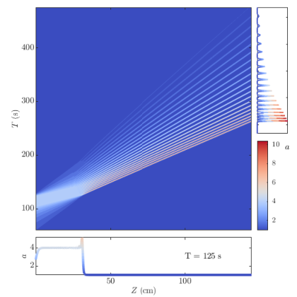
Utilizing the theoretically prescribed boundary condition (20) that results in the step profile (5) at for the solution of the dispersionless equation with unit step initial condition, we perform numerical simulations of the full conduit equation (4) and carry out fluid experiments. A typical numerical simulation is depicted in the contour plot of Fig. 3. The wave profile steepens until dispersion becomes important, coinciding with the emergence of oscillations, which prevent the formation of a discontinuity. Nevertheless, using the method described in the previous section to extract from the simulations, the observed breaking locations and times are within 3.75% and 1.35% relative error, respectively of their predicted values across a range of step ratios and breaking heights as depicted by the triangles and dashed lines in Fig. 7.
For the experiment, thirteen trials were taken over the course of four hours. The main results of this experiment are also shown in Fig. 7. The predicted breaking heights and times ( and ) (denoted with dashed lines) are very close to the experimentally observed values ( and ) (denoted by squares). Figure 7 includes the theoretical prediction, numerical simulations, and experiment for the breaking height (a) and the breaking time (b). All experiments were under relative error in breaking height and relative error in breaking time . Therefore, a high degree of wavebreaking control is achieved by our approach. Furthermore, the prediction’s accuracy appears to be independent of the breaking amplitude , which is consistent with the dimensional analysis requirement (9) that is independent of wave amplitude.
These observations extend previous experimental comparisons of theoretical predictions for the conduit equation involving solitons Scott et al. 1986; Olson and Christensen 1986; Helfrich and Whitehead 1990; Lowman et al. 2013 and dispersive shock waves Maiden et al. 2016; Maiden et al. 2018—i.e., nonlinear, dispersive waves—into the non-dispersive, nonlinear regime. It is noteworthy that theoretical predictions derived from the relatively simple inviscid Burgers model, , agree so well with numerical simulations and experiment across a range of parameter values.

III.4 Results for Triangle, N, and Box Profiles
Experiments were also performed for other wavebreaking profiles. Experiments on boundary conditions for generating triangle waves (22) and N-waves (24) showed good fidelity to the expected shapes, as shown in Fig. 8. Moreover, we obtain quantitative agreement between the predicted characteristics (recall Fig. 1(c,d)) and the observed curves of equi-area pre-breaking as shown by the dashed lines overlayed on the cross-sectional area contour plot. For the figure, we fit and to those found experimentally, then generated the predicted characteristics (contours) based on these values. We find this fitting method is equivalent to fitting to the data, similar to what was done for the step profile.
As an application of our approach to generating desired wave profiles at breaking, we show an experimental and numerical realization of solitary wave fission Trillo et al. from the long-time dynamics of a box profile in Figs. 9(a) and 9(b), respectively. The boundary time-series for the box profile, eq. (21), results in an approximately rectangular-shaped area profile with a specified width and height. The long-time evolution of this profile results in a train of solitary waves. The numerical simulation in Fig. 9(b), generated by the same boundary control procedure, exhibits excellent agreement with the experiment in Fig. 9(a) for the experimental volumetric flow rate if we introduce the fitted values and (measured values and ). Future work aims to explore the post-breaking dynamics of this and other dispersive hydrodynamic problems by leveraging the boundary control method introduced here.
IV Conclusion
While previous experimental and theoretical work on the conduit equation and its corresponding viscous two-fluid system have primarily focused on dispersive hydrodynamics post-breaking, i.e., when nonlinearity and dispersion are important, this work considers the simpler case of very long waves where nonlinearity dominates the flow. A simple long-wave hyperbolic model (the inviscid Burgers equation) is used to theoretically control nonlinear wave propagation at the interface of a viscous fluid conduit prior to wavebreaking. The pre-breaking validity of the hyperbolic model enables the precise creation of desired wavebreaking profiles in the interior of the dispersive hydrodynamic domain with only boundary control. Characteristics are propagated backward in time from a desired wave profile until they reach the boundary. So long as the backward characteristics do not overlap, it is possible to obtain a bounday condition whose forward propagation approximately results in the desired wavebreaking profile.
In order to compare this dispersionless theory with the “dispersionfull” conduit equation and experiment, we define wavebreaking by an inflection point criterion for the wavefront’s slope. This definition provides a bridge between the long-wave, pre-breaking dynamics and the short-wave oscillations that emerge post-breaking. Most importantly, we obtain quantitative agreement between theory, numerical simulation, and experiment with this wavebreaking definition. For a step profile, the observed breaking heights and times are within and , respectively, of their expected values. For more complex profiles—the triangle and N-wave configurations—we obtain good characteristic control observed in measured space-time contour plots. One example of post-breaking dispersive hydrodynamics is highlighted where a large number of solitary waves emerges from a large box profile. Numerical simulation and experiment utilizing the same box profile boundary condition result in striking agreement and motivate further analysis of the soliton fission problem in the context of the viscous fluid conduit system. The relatively simple characteristic method proposed here holds promise for other dispersive hydrodynamic media.
References
- El and Hoefer (2016) G. A. El and M. A. Hoefer, “Dispersive shock waves and modulation theory,” Physica D: Nonlinear Phenomena 333, 11 – 65 (2016).
- Olson and Christensen (1986) P. Olson and U. Christensen, “Solitary wave propagation in a fluid conduit within a viscous matrix,” Journal of Geophysical Research: Solid Earth 91, 6367 (1986).
- Lowman and Hoefer (2013) N. K. Lowman and M. A. Hoefer, “Dispersive hydrodynamics in viscous fluid conduits,” Phys. Rev. E 88, 023016 (2013).
- Whitehead and Helfrich (1988) J. A. Whitehead and K. R. Helfrich, “Wave transport of deep mantle material,” Nature 336, 59 (1988).
- Maiden and Hoefer (2016) M. D. Maiden and M. A. Hoefer, “Modulations of viscous fluid conduit periodic waves,” Proc. Royal Soc. Lond A: Mathematical, Physical and Engineering Sciences 472 (2016), 10.1098/rspa.2016.0533.
- Scott et al. (1986) D. R. Scott, D. J. Stevenson, and J. A. Whitehead, “Observations of solitary waves in a viscously deformable pipe,” Nature 319, 759–761 (1986).
- Helfrich and Whitehead (1990) K. R. Helfrich and J. A. Whitehead, “Solitary waves on conduits of buoyant fluid in a more viscous fluid,” Geophysical & Astrophysical Fluid Dynamics 51, 35–52 (1990).
- Lowman et al. (2013) N. K. Lowman, M. A. Hoefer, and G. A. El, “Interactions of large amplitude solitary waves in viscous fluid conduits,” Journal of Fluid Mechanics (2013).
- Maiden et al. (2016) M. D. Maiden, N. K. Lowman, D. V. Anderson, M. E. Schubert, and M. A. Hoefer, “Observation of dispersive shock waves, solitons, and their interactions in viscous fluid conduits,” Phys. Rev. Lett. 116, 174501 (2016).
- Maiden et al. (2018) M. D. Maiden, D. V. Anderson, N. A. Franco, G. A. El, and M. A. Hoefer, “Solitonic dispersive hydrodynamics: Theory and observation,” Phys. Rev. Lett. 120, 144101 (2018).
- Trillo et al. (2016) S. Trillo, M. Klein, G. F. Clauss, and M. Onorato, “Observation of dispersive shock waves developing from initial depressions in shallow water,” Physica D: Nonlinear Phenomena 333, 276 – 284 (2016), dispersive Hydrodynamics.
- Xu et al. (2017) Gang Xu, Matteo Conforti, Alexandre Kudlinski, Arnaud Mussot, and Stefano Trillo, “Dispersive dam-break flow of a photon fluid,” Phys. Rev. Lett. 118, 254101 (2017).
- Janantha et al. (2017) P. A. Praveen Janantha, Patrick Sprenger, Mark A. Hoefer, and Mingzhong Wu, “Observation of self-cavitating envelope dispersive shock waves in yttrium iron garnet thin films,” Phys. Rev. Lett. 119, 024101 (2017).
- Chong et al. (2017) C. Chong, M. A. Porter, P. G. Kevrekidis, and C. Daraio, “Nonlinear coherent structures in granular crystals,” Journal of Physics: Condensed Matter 29, 413003 (2017).
- Wetzel et al. (2016) Benjamin Wetzel, Domenico Bongiovanni, Michael Kues, Yi Hu, Zhigang Chen, Stefano Trillo, John M. Dudley, Stefano Wabnitz, and Roberto Morandotti, “Experimental generation of riemann waves in optics: A route to shock wave control,” Phys. Rev. Lett. 117, 073902 (2016).
- Whitham (1965) G. B. Whitham, “Non-linear dispersive waves,” Proc. Royal Soc. Lond A: Mathematical, Physical and Engineering Sciences 283, 238 (1965).
- (17) S. Trillo, G. Deng, G. Biondini, M. Klein, G. F. Clauss, A. Chabchoub, and M. Onorato, “Experimental Observation and Theoretical Description of Multisoliton Fission in Shallow Water,” 117, 144102.
- (18) N. Ghofraniha, L. Santamaria Amato, V. Folli, S. Trillo, E. DelRe, and C. Conti, “Measurement of scaling laws for shock waves in thermal nonlocal media,” 37, 2325–2327.
- Whitehead and Luther (1975) J. A. Whitehead and D. S. Luther, “Dynamics of Laboratory Diapir and Plume Models,” Journal of Geophysical Research 80, 705–717 (1975).
*
Appendix A Boundary Conditions for Wavebreaking Profiles
All following profiles have a breaking time based on the breaking height of .
The boundary condition resulting in an approximate step profile for (4) (see Fig. 1a)
| (20) |
For a box, this profile is cut off at the time of breaking (see Fig. 1b)
| (21) |
For a right triangle with height , width , and hypotenuse slope , once the maximum desired height is reached, we begin decreasing the flow rate in a way consistent with Eq.(14) (see Fig. 1c)
| (22) |
The width-height restrictions on the triangle wave are based on having the triangle fully in the conduit at the time of breaking as well as the non-breaking condition
| (23) |
For an N-wave with maximum height , minimum height , width , and slope , we generate a triangle wave whose final area dips below the mean flow rate down to before returning to the mean flow (see Fig. 1d)
| (24) |
The N-wave width-height restrictions are also based on having the wave fully in the conduit at the time of breaking and the non-breaking condition
| (25) |
Note when and , we arrive at Eq. (17).