Conditional probabilities in multiplicative noise processes
Abstract
We address the calculation of transition probabilities in multiplicative noise stochastic differential equations using a path integral approach. We show the equivalence between the conditional probability and the propagator of a quantum particle with variable mass. Introducing a time reparametrization, we are able to transform the problem of multiplicative noise fluctuations into an equivalent additive one. We illustrate the method by showing the explicit analytic computation of the conditional probability of a harmonic oscillator in a nonlinear multiplicative environment.
I Introduction
Stochastic dynamics driven by multiplicative noise is, by now, a common arena to model complex behavior Gardiner 1996; van Kampen 2007. In fact, several very different areas of knowledge have benefited from stochastic modeling, such as physics and chemistry Freund and Pöschel 2000, biology and ecology Murray 2002 and even economy and social sciences Mantegna and Stanley 2000; Bouchaud and Potters 2003. From a physical perspective, multiplicative stochastic dynamics is one of the possible approaches to enhance our understanding of out-of-equilibrium statistical mechanics Crooks 1999; Zwanzig 2001; Seifert 2008.
Some typical examples of multiplicative noise processes are the diffusion of particles near a wall Lançon et al. 2001; Lançon et al. 2002; Lau and Lubensky 2007; Volpe et al. 2010; Brettschneider et al. 2011, micromagnetic dynamics in ferromagnetic systems García-Palacios and Lázaro 1998; Aron et al. 2014; Arenas et al. 2018 and non-equilibrium transitions into absorbing states Hinrichsen 2000. Moreover, among the very interesting stochastic phenomena described by multiplicative noise, there are two particular ones: noise-induced phase transitions Van den Broeck et al. 1994; Castro et al. 1995; Carrillo et al. 2003; Jafarpour et al. 2015; Barci et al. 2016 and stochastic resonance Benzi et al. 1981; Benzi et al. 1983; Wio, H. S. and Deza, R. R. 2007; Wio et al. 2002, in which the interplay between nonlinearity and noise produces surprising outputs.
There are several theoretical approaches to deal with this type of processes. The choice of any particular one mainly depends on what kind of observables we are interested in and what kind of calculation technique we are willing to apply. For instance, the Langevin approach, consisting in a system of stochastic differential equations, is the natural way to model a specific situation and to perform numerical simulations Sivak et al. 2014. By the other hand, we can gain more insightful intuition by looking at the Fokker-Planck equation, which directly provides the time dependent probability distribution. Other analytic approaches, such as mean fields, perturbation theory and even renormalization group techniques are also available Goldenfeld 1992. Moreover, the path integral formulation of stochastic processes is quite useful to compute correlation and response functions Wio 2013. Even though path integrals for multiplicative noise processes have been studied for a long time Janssen 1992, important progresses have been recently reached Aron et al. 2010; Arenas and Barci 2010; Arenas and Barci 2012a; Arenas and Barci 2012b; Moreno et al. 2015; Aron et al. 2016. Interestingly, this technique provides a useful and beautiful connection between a classical stochastic process and a quantum mechanical problem Zinn-Justin 2002.
Preparing the system at a certain time with a probability density distribution , the solution of the Fokker-Planck equation provides a time-dependent probability distribution, , at any time . Equivalently, it can be written in the form
| (1) |
where is the conditional probability distribution of the variable at a time , provided it was at a previous time .
The conditional probability is a central object in the theory of stochastic processes since it contains detailed information about dynamics. For instance, equilibrium properties, such as detailed balance, can be cast in terms of the conditional probability and its time reversal. A careful definition of the time reversal conditional probability, detailed-balance relations, as well as microscopic reversibility in multiplicative processes was developed in Ref. Arenas and Barci 2012b.
The explicit computation of the conditional probability is quite involved. One of the methods to compute it is based in its path integral representation. For an additive noise Langevin equation, the problem is equivalent to the computation of a propagator of a quantum particle. In this context, perturbation theory or semi-classical expansions Caroli et al. 1979; Caroli et al. 1981 can be implemented.
In this paper, we propose a method to analytically compute a weak noise expansion of the conditional probability in the case of a multiplicative process driven by a Langevin equation. We show that, when written in its path integral representation, its computation is equivalent to compute a propagator of a quantum particle with variable mass. The state-dependent diffusion is translated to a quantum equivalent model as a space-dependent mass. The quantization of a classical model with variable mass is not uniquely defined Sá Borges et al. 1988, since the kinetic term is a product of non-commuting (coordinate and momentum) operators. This ambiguity resembles, in the stochastic process, different discretization prescriptions needed to properly define the stochastic differential equation. We describe a method to compute a weak noise expansion of the conditional probability in an arbitrary stochastic prescription. The key point, in order to compute fluctuations, is the introduction of a reparametrized time that transforms the structure of the fluctuation operator with multiplicative noise into a simpler form, typically displayed in additive noise problems. In some sense, we are transforming multiplicative noise into additive noise by means of a time reparametrization. This is different from the usual way to transform multiplicative into additive noise, by means of a nonlinear variable transformation Gardiner 1996; van Kampen 2007; Itô 1951. Using this technique, fluctuations can be explicitly computed in the reparametrized time. In the end, it is necessary to invert the time transformation in order to have sensible results.
To illustrate the technique we show a simple nontrivial example. We compute the conditional probability of an overdamped harmonic oscillator in the presence of a (nonlinear) multiplicative noise. We obtain analytic results, allowing to explore the behavior of the conditional probabilities in different time regimes. Ir order to check the accuracy of the method we compare our results with numerical solution of the Fokker-Planck equation.
The paper is organized as follow: in section II, we describe the model and set up the basic notation we use all along the paper. In § III we show that the conditional probability of a multiplicative stochastic process is equivalent to the propagator on a quantum particle with position-dependent mass. In section IV, we describe a weak noise expansion or semi-classical approximation. Here, we introduce the time reparametrization that allows us to compute fluctuations. Finally, in § V we show a particular example to illustrate how the computational technique is applied. We discuss our results in § VI. Additionally, we show details of the calculation in two appendices.
II Langevin description of a multiplicative white noise stochastic evolution
In order to describe the model and to set up notations, we briefly review in this section the Langevin and Fokker-Planck description of the dynamical evolution of a multiplicative white noise stochastic process.
We consider a single random variable satisfying a first order stochastic differential equation given by
| (2) |
where is a Wiener process. Thus, obeys a Gaussian white noise distribution with
| (3) |
measures the noise intensity while and are arbitrary smooth functions of , representing the drift force and the square root of the diffusion function, respectively. To completely define equation (2) we fix the generalized Stratonovich Hänggi 1978 prescription (also known as prescription Janssen 1992) to define the stochastic integrals. In this prescription, the integrals are defined by the discretization rule
| (4) |
where is chosen from
| (5) |
The limit in Eq. (4) is understood in the sense of mean-square limit Gardiner 1996. The solutions of Eq. (2) depends on the particular value of . Two popular choices are , that corresponds with the pre-point Itô interpretation, and , with the (midpoint) Stratonovich one. Different values of also imply different calculus rules. The most striking property is the chain rule. For an arbitrary function of the stochastic variable, , it takes the form Arenas and Barci 2012a; Arenas and Barci 2012b,
| (6) |
As a consequence, integration by parts should be performed with great care. Clearly, for , equation (6) is the usual chain rule. In fact, the Stratonovich prescription is the only one in which all the usual calculus rules are preserved. Sometimes, it is useful to represent the same stochastic process in different prescriptions. For instance, if the process is defined by Eq. (2) in the prescription, the same process can be formulated in another prescription by shifting the drift force as
| (7) |
where , (a rigorous demonstration can be found in the appendix of Ref. Moreno et al. 2015), Using this relation, it is sometimes useful to consider, instead of Eq. (2) defined in the prescription, the alternative equation
| (8) |
with
| (9) |
where, now, the discretization is taken in the Stratonovich prescription. In this way, solutions of Eq. (8), solved in the Stratonovich convention, coincide with those of Eq. (2), solved in the -prescription (with arbitrary ).
Eq. (2) or, equivalently, Eq. (8), leads Lau and Lubensky 2007 to the Fokker-Planck equation
| (10) |
where is the time-dependent probability distribution and the probability current is given by
| (11) |
This equation has a time independent equilibrium solution which satisfies . It has the form
| (12) |
where is a normalization constant and
| (13) |
In most practical cases, in the absence of noise, the system is conservative, characterized by a potential . In these cases, the relation between the drift force and the potential is
| (14) |
that can be considered as a generalization of the Einstein relation for Brownian motion to the case of multiplicative noise Arenas and Barci 2012b. Replacing Eq. (14) into Eq. (13) we find for the equilibrium potential
| (15) |
The equilibrium distribution depends not only on the given functions , but also on the value of the -prescription which defines the Wiener integral. The only prescription that leads to the Boltzmann distribution is ; for this reason, this convention is sometimes called “thermal prescription” or even Hänggi-Klimontovich interpretation Hänggi and Thomas 1982; Klimontovich 1994. Furthermore, this prescription is also known as anti-Itô interpretation. Interestingly, it can be considered as the time reversal conjugated to the Itô prescription Arenas and Barci 2012b; Moreno et al. 2015.
Choosing convenient values for and , it is possible to study, in a unified formalism, model systems with general equilibrium distributions that go from Boltzmann thermal equilibrium to power-law distributions. A simple example of the latter case is to consider a pure noisy system with . In that case, the equilibrium distribution is .
III Classical stochastic evolution and quantum mechanics of a particle with variable mass
The transition probability is a central ingredient in the study of any dynamical property of a stochastic process. It represents the conditional probability of finding the system in the state at time , provided the system was in the state at time . In the path integral formalism, it can be written as Arenas and Barci 2010
| (16) |
where the “action” is given by
| (17) |
with boundary conditions and . Eqs. (16) and (17) are the Onsager-Mashlup representation Onsager and Machlup 1953 of the transition probability of the stochastic process driven by Eq. (8). Note that, for simplicity, we have built a path integral representation of Eq. (8). In this way, we can employ usual calculus rules to deal with the path integral. The information about the different stochastic prescriptions is codified in , given by Eq. (9). Alternatively, we could choose to represent Eq. (2) in the past integral formalism; in this case, it would be necessary to use the -generalization of stochastic calculus Arenas and Barci 2012b; Moreno et al. 2015. Of course, the results are exactly the same, the chosen representation is just a matter of convenience.
It is instructive to rewrite the action in an alternative way. Expanding the squared bracket in Eq. (17), using Eqs. (9) and (14) and integrating by parts, we find
| (18) |
Here, the first term is a state function governed by the equilibrium potential evaluated at the initial and the final state of the system, , with given by Eq. (15). The Lagrangian can be written in the suggestive form,
| (19) |
where
| (20) |
The primes, , means derivative with respect to . Replacing Eq. (18) into Eq. (16), the conditional probability takes the form
| (21) |
where the propagator is given by
| (22) |
Here, the functional integration measure is
| (23) |
where , with and .
Interestingly, Eq. (22) is the exact propagator of a quantum particle with position-dependent mass moving in a potential , written in the imaginary time path integral formalism . The noise places the role of in the quantum theory. There is subtlety in the identification of the stochastic and the quantum problem. Inside , Eq. (20), there are terms of order and . These terms are absent in a pure quantum problem, where the potential is independent of . However, as we will show in next section, this fact is important in developing a weak noise (or semi-classical) approximation since the saddle-point approximation has contributions of the same order than fluctuations.
The quantization of a classical system with variable mass has ambiguities due to operator ordering. In fact, the quantum kinetic term mixes the non-commuting operators, position and momentum . As a consequence, different orderings in the Hamiltonian are not equivalent. In the configuration space path integral approach, this fact is reflected in different discretization schemes of the time integral. Then, the quantum ordering problem is associated in the classical Langevin description with the different stochastic prescriptions available to compute the Wiener integrals. Specifically, the propagator of Eq. (22) with time integrals symmetrically discretized (Stratonovich prescription ), is equivalent to a quantum problem described by a Hamiltonian operator with the Weyl order Sá Borges et al. 1988,
| (24) |
It is worth mentioning that, in our formalism, the dependence of the conditional probability on the stochastic prescription is completely taken into account through the expression of the equilibrium potential , given by Eq. (15).
In the next section, we present a detailed procedure for analytically computing the propagator of Eq. (22) in a weak noise expansion.
IV Weak noise expansion
In order to explicitly compute the conditional probability, we make a weak noise expansion, in some sense, equivalent to a semi-classical (or WKB) approximation in quantum mechanics. The general method is very well known in additive noise processes and in quantum systems. The main idea is that the functional integral of Eq. (16) is dominated, at very low noise, by extrema of the action, in such a way that at first approximation
| (25) |
where (with ) are different solutions of the classical equation of motion with the same boundary conditions. To improve the approximation, the functional integral of Eq. (16) could be computed considering small fluctuations around each solution . This integration produces a prefactor in Eq. (25) given in terms of a functional determinant (see below) that, upon exponentiation, will result in an effective action containing terms proportional to (or in a quantum system). The application of this procedure to multiplicative stochastic processes or, equivalently, to variable mass quantum problems, is cumbersome Langouche et al. 1979. In particular, we will see that the classical solution as well as fluctuation contributions to the effective action, both have -dependent terms. Thus, it will be necessary to carefully compute and consider both contributions in order to get a consistent approximation.
In this section, we present a general procedure for the computation of the conditional probability in a stochastic process driven by a drift force and a diffusion function , for a general stochastic prescription .
We begin by assuming that, at very weak noise, the functional integral, Eq. (16) is dominated by the solutions of the classical equation , where is given by Eq. (18). Explicitly computing the functional derivative, we find
| (26) |
This equation provides an alternative interpretation of the classical problem. It corresponds with the classical dynamics of a unit mass particle, moving under the influence of a non-conservative velocity dependent force, proportional to Sá Borges et al. 1988. This term is proper of multiplicative systems since it is proportional to . The solution of Eq. (26) is quite involved due, on one hand, to the nonlinearity introduced by the diffusion function and, on the other, to the nonlinearity in the velocity. However, using the fact that the Lagrangian is invariant under time translations, it is not difficult to built up a first integral of this equation. In fact, the canonical momentum and the classical Hamiltonian can be simply computed, obtaining
| (27) |
This is a classical Hamiltonian, thus, there is no ordering problem of the kinetic term. The Hamiltonian, evaluated on a solution of the equation of motion
| (28) |
should be a conserved quantity, . Then,
| (29) |
where and . Note that the Hamiltonian, even though it is a conserved quantity, is not the energy, since the Lagrangian is not a homogeneous quadratic function of the velocity.
From Eq. (29), we can write the solution of Eq. (26) by a quadrature
| (30) |
where we have defined an effective potential
| (31) |
These expressions have two arbitrary constants, and , that should be determined by means of the boundary conditions and . Thus, Eqs. (30) and (31) implicitly define , used as a starting point of the weak noise approximation. As anticipated, due to the fact that contains terms proportional to (see Eq. (20)), will contain such terms. Therefore, for consistency, we need to go beyond the saddle-point approximation. The following subsection is devoted to this matter.
IV.1 Reparametrization of time and Gaussian fluctuations
Let us assume, for the moment, that, given initial and final conditions, the classical solution is unique. The generalization to multiple solutions is straightforward. Then, we consider fluctuations around it
| (32) |
with boundary conditions . Replacing the expansion into Eq. (22) and keeping up to second-order terms in the fluctuations we find for the propagator
| (33) | ||||
where the classical action is
| (34) |
and the fluctuation kernel
| (35) |
In Eq. (33), the functional integration measure is
| (36) |
Although Eq. (33) formally looks like a Gaussian integral, its evaluation is not simple. The reason is twofold. On one hand, the fluctuation kernel , Eq. (35), is not trivial due to the time dependence of . On the other, the integration measure, Eq. (36), has the diffusion function in the denominator. This factor comes from in Eq. (16) and resembles curvature effects in the time axes.
In order to compute the fluctuation integral, we make a time reparametrization. For concreteness, we introduce a new time variable , by means of
| (37) |
This is a nontrivial local scale transformation, weighted by the diffusion function, evaluated at the classical solution . Eq. (37) defines a function , in such a way that
| (38) |
We have chosen the integration constant in order to keep the time origin unchanged, .
Performing this time reparametrization, the fluctuation kernel transforms as , and takes the simpler form
| (39) |
where
| (40) |
On the other hand, after discretizing the reparametrized time axes , the functional integration measure, Eq. (36) becomes
| (41) |
in which the function has been absorbed in the reparametrization.
Thus, in the new time variable , the functional integral of fluctuations is Gaussian and can be formally evaluated, obtaining for the propagator
| (42) |
where the relation between and is given through Eq. (37).
Considering that Eq. (42) is the main result of this section, let us comment on its meaning. The general formal structure of the propagator is the usual one in a semiclassical approximation. It consists on an exponential of a classical action and a prefactor which codifies fluctuations. However, in the present case of multiplicative noise processes, there are important differences that we should stress. One of the effects of the multiplicative noise in the classical action is to correct terms proportional to and to produce new terms of order , as can be seen from the definition of the potential , Eq. (20). Thus, in order to correctly implement the approximation scheme, it is essential to compute fluctuations, since they will contribute with terms of the same order. The explicit computation of the prefactor is very interesting. The transformed fluctuation operator , Eq. (39), has exactly the same structure as the fluctuation operator of an additive process, albeit with a modified potential , Eq. (40). This fact allows us to compute the functional determinant using the usual techniques developed to treat additive noise. However, the result of this computation is expressed in a reparametrized time variable . In order to produce sensible results, at the end of the calculations, we need to go back to real time, , by inverting the reparametrization transformation. Summarizing, we have transformed the computation of fluctuations in a multiplicative stochastic process into a simpler problem of an additive process by means of a time reparametrization.
V Transition probability for an overdamped harmonic oscillator with multiplicative noise
In this section, we illustrate the method proposed in this paper by analyzing the simplest nontrivial example of a multiplicative stochastic process. Let us consider an overdamped harmonic oscillator in the presence of multiplicative noise. A lot of particular examples of this system have been analyzed for different physical applications. A good pedagogical presentation with lots of references can be found in Ref. Gitterman 2005. Much of these references try to compute the Fokker-Planck equation or some moments of the probability distribution. Differently, we are interested here in the transition probability with the main purpose of explicitly showing how the technique described in this paper (specially the time reparametrization) works.
For concreteness, let us choose a harmonic oscillator potential
| (43) |
where is the natural frequency of the oscillator and a diffusion function
| (44) |
where controls the intensity of the multiplicative component of the noise. In particular, for , we recover the usual additive white noise process.
Using the generalized Einstein relation, Eq. (14), the drift force is
| (45) |
This relation guarantees that the equilibrium potential, Eq. (15), is given by
| (46) |
implying, for the asymptotic equilibrium probability distribution,
| (47) |
where is a normalization constant. One of the effects of multiplicative noise is to correct the Gaussian equilibrium distribution with a power law factor which depends on the stochastic discretization prescription . We also observe that, for the Hänggi-Klimontovich prescription (), the equilibrium probability distribution is of Boltzmann type, completely equivalent to a harmonic oscillator with additive noise.
We want to compute the propagator for this model in the weak noise approximation by using Eq. (42), where we have chosen initial conditions , , and final conditions , .
The first step in the weak noise approximation is to compute the classical action . To do this, we need to compute the solution of the saddle-point equation, Eq. (26) or, equivalently, Eq. (30), and to replace it into Eq. (34). We have computed considering a weak multiplicative effect, . That is, the results are accurate in a distance range, , where the diffusion function is not very far from its additive value . For details of the calculations, Appendix A can be consulted. We have obtained
| (48) |
The first line of this expression is the usual result for the harmonic oscillator with additive noise. The second line is the correction due to the multiplicative noise to order . For very weak noise, only the first term of Eq. (48) is relevant. An important observation is that we are getting terms of order at saddle-point level. On the other hand, fluctuations will contribute also with terms. Consequently, this approximation is only consistent provided fluctuations are taken into account.
As described in the preceding section, to properly compute fluctuations we need to reparametrize the time variable according to Eq. (37). In the present example, this reparametrization reads
| (49) |
where . With this reparametrization the computation of fluctuations reduces to evaluating the determinant of the operator of Eq. (39), where we have, now,
| (50) |
In Appendix B, we explicitly compute this determinant in the reparametrized time axes and, after that, we turn back to original time variable . The result at order is
| (51) |
Since Eq (51) is an expansion in , we can exponentiate the second term and absorb it in the definition of an effective action, finally obtaining for the propagator
| (52) |
where
| (53) |
This is the central result of this section. We have computed, in closed analytic form, the propagator for a harmonic oscillator under the influence of a nonlinear multiplicative noise in the weak noise approximation. The first term of Eq. (53) is the usual result for a harmonic oscillator under additive noise, while the second term represents the corrections due to the multiplicative character of the noise.
It is instructive to analyze particular limits in the time scale. For instance, consider . In this case, Eq. (53) takes the simpler form
| (54) |
The first term is the result for a diffusive free particle. This is, indeed, the correct result since, for very short times, the particle did not have enough time to explore the harmonic potential. The first correction in is due to multiplicative noise (order ) and is independent of the stochastic prescription; -dependent terms only appear at order .
On the other hand, in the asymptotic limit , the effective action is
| (55) |
Replacing this result into Eq. (52) we get, for the conditional probability Eq. (21),
| (56) |
which is the correct result obtained, independently, by solving the stationary Fokker-Planck equation.
V.1 Comparison with the exact Fokker-Planck solution
In order to check the method and the accuracy of our approximation, we compare the analytic result with the numerical solution of the Fokker-Planck equation. In fact, from Eq. (1), it is simple to check that the conditional probability is the solution of the Fokker-Planck equation, , with the initial condition . Therefore, we numerically solved equations (10) and (11), for our model Eqs. (43) and (44). In Figure 1, we depict a solution for typical values of the parameters, , , and .

The initial probability density is strongly peaked at . It diffuses in time and, at long times, saturates to the exact analytic expression Eq. (47). We observe that, as already commented, the asymptotic equilibrium probability depends on the stochastic prescription . For anti–Itô prescription, , the probability density is Gaussian. However, for , the Gaussian behavior is slightly corrected by a power law. In the region , the distribution can be approximated by a Gaussian with variance . This behavior, deduced from Eq. (47), is verified by the numerical solution of the Fokker-Planck equation with great precision. On one hand, we see that the effect of the multiplicative character of the noise is controlled by the parameter . We also note from Figure 1 that, for , the asymptotic limit is already reached. On the other hand, our approximate analytic result, valid for and , can be written in the form of a normal distribution,
| (57) |
where the dimensionless time-dependent variance is given by
| (58) |
The first term in the last expression corresponds to the usual additive noise result, while the second one, proportional to , is the multiplicative noise correction. From this equation, it is immediate to verify that in the asymptotic limit , we get the correct result , while at very short time approximation, , we reach the initial distribution .
Now, we compare the approximate analytic solution with the exact numerical distribution in all the time range for different values of the parameters. For this, we observe that the variance can be obtained from the maximum of the distribution probability at , as . In the same way, we define the quantity
| (59) |
computed from the numerical solution, , of the Fokker-Planck equation. In Figure 2, we depict both curves computed in the Itô prescription, , with a moderate value of the noise and . We see that both curves coincide in the range within the graphic precision.

Although we are working in the weak noise approximation, Eq. (58) is quite accurate even for noise intensities as big as .
In Figure 3, we show two curves computed with the same parameters values , , but for different stochastic prescriptions.


We see that the curves fit quite well for initial values of the time evolution as well as in the asymptotic limit. In the intermediate range, we begin to observe a small deviation due to the big value of the noise. It can also be noticed from this figure that a better approximation is obtained for the Hänggi-Klimontovich interpretation ().
We quantified the observed deviation by computing the difference for different stochastic prescriptions. In Figure 4, we depict for and . The dot-dashed curve was computed in the Itô prescription (), the solid line was evaluated in the Stratonovich prescription () and the anti-Itô interpretation () is shown by the dashed line.
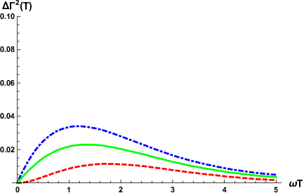
Clearly, although the errors are very small for these values of the parameters, we get our best result in the anti-Itô prescription. The reason is that in this prescription, the exact asymptotic probability density is Gaussian, the same one of our approximation. The exact asymptotic expression for any other value of is, in general, not Gaussian. This fact is reflected in Figure 4, in the residual values of the curves for .
VI Discussion and conclusions
In this paper, we have analyzed the weak noise approximation for computing conditional probabilities in a multiplicative stochastic process. We noted that this problem is equivalent to compute the propagator of a quantum problem which describes a particle with variable mass in an external potential. Indeed, the diffusion function , in the classical stochastic model, plays the role of the inverse mass in the quantum equivalent problem (). On the other hand, the necessary stochastic prescriptions used to properly define the Wiener integral have their counterpart in the ordering problem in quantum mechanics. The position-dependent mass mixes non-commuting operators ( and ) in the kinetic term of the Hamiltonian. In the stochastic process, the Stratonovich prescription is equivalent to the Weyl order for the quantum associated problem. In this paper, we have presented the computation of the propagator using a ”generalized Stratonovich prescription”, parametrized by a continuous parameter , which contains the most popular stochastic interpretations as particular cases.
The direct implementation of the usual weak noise, or semi-classical, approximation for this type of systems is quite involved. In fact, when performing the saddle-point approximation plus quadratic fluctuations, we see that fluctuations are not Gaussian, due to the multiplicative noise effects on the functional integration measure. On the other hand, the fluctuation operator is very elaborate because of the time dependence of the diffusion function (or equivalently, the mass). To solve this problem and to effectively integrate fluctuations, we have performed a time reparametrization weighted with the diffusion function, computed at the classical solution of the equation of motion, . The net effect is to transform the problem of computing fluctuations of a multiplicative process into an equivalent additive noise problem. This is one of the main contributions of this paper.
The transformation of a multiplicative noise process into an equivalent additive one can be done, at least for a single variable, by means of a nonlinear transformation of the stochastic variable. This fact is very well known and gives rise to all the subtleties of different types of stochastic calculus. In higher dimensions, this transformation can be done only in very particular cases and it is quite problematic in the context of the path integral representation, even in one dimension Cugliandolo and Lecomte 2017. The transformation we have presented in this paper is of a different type, since it is not a variable transformation, but a local time reparametrization. Interestingly enough, a similar, however different, type of time reparametrization was previously used in the context of path integral to relate the harmonic oscillator propagator with the free particle propagator Moriconi 2004.
In some sense, what we are doing is rectifying the multiplicative character of the noise by locally changing the way we measure time. A similar related idea was recently proposed in Ref. Rubin et al. 2014. In that reference, a time reparametrization equivalent to Eq. (37) was proposed, but keeping the stochastic character of the variable . In this way, a new “stochastic time” was introduced, allowing to change the multiplicative process into an additive one. Differently, in our approach, the time transformation, Eq. (37), is not stochastic since the diffusion function is evaluated at the solution of the saddle-point equation. The classical solution provides a well-defined protocol to rectify the multiplicative noise. Of course, this procedure works for computing quadratic fluctuations. Probably, it would be necessary to correct it, order by order, if we pretend to compute higher order fluctuations. An additional advantage of the time reparametrization technique is that it can be straightforwardly implemented in higher dimensional systems.
We illustrated the procedure by showing the explicit computation of the propagator of the simplest nontrivial model. We have considered an overdamped harmonic oscillator with nonlinear multiplicative noise. We have solved the saddle-point equation in the weak multiplicative noise regime and we computed fluctuations using the proposed time reparametrization. We showed how the multiplicative noise affects the conditional probability and we have shown short and long times limits in order to check the results. We have also compared the analytic approximate propagator with the numerical solution of the Fokker-Planck equation finding an excellent match, even well beyond the parameters region where the approximation is expected to work.
Having this powerful technique in hands, it is now possible to attack more involved problems, such as a potential with several minima, in order to address problems like stochastic resonance in systems with multiplicative noise. We hope to report on this subject in the near future.
Appendix A Saddle-point approximation
The first step in the weak noise approximation is to solve the saddle-point equation, Eq. (26) or, equivalently, Eq. (30). By using the expression for the equilibrium potential given by Eq. (46), we can build from Eq. (20). It can be approximated as
| (60) |
where, in the spirit of the weak noise approximation, we have kept terms up to order . We have also considered a weak multiplicative effect, . That is, we compute the potential in a distance range , where the diffusion function is not very far away from its additive value . In the same approximation, we compute from Eq. (31), obtaining
| (61) |
with
| (62) |
With this expression for , we solve Eq. (30), with the boundary conditions and . We immediately find the classical solution
| (63) |
In order to have a completely defined solution, we need to determine the constant , contained in the frequency . To determine it, we observe from Eq. (29) that . Using the solution Eq. (63) we obtain the transcendental equation
| (64) |
The solution of equations (62) and (64) for and completely determines the classical solutions , Eq. (63). Although this equation can only be solved numerically, we observe that, within the range of our approximation, an analytic expression can be found. Using a perturbative recurrent procedure, we find, to order ,
| (65) | ||||
| (66) |
Now, we are in condition to compute from Eq. (34). Using Eq. (29) we find the simpler equation
| (67) |
Replacing into Eq. (67), performing the time integral and using the expressions of Eqs. (65) and (66), we find to quadratic order in ,
| (68) | ||||
The first line of Eq. (68) is the usual result for the classical action of the harmonic oscillator. The second line, proportional to , codifies information about the multiplicative noise.
Appendix B Fluctuations
To compute fluctuations, we need to evaluate the prefactor in Eq. (42), , where is the time reparametrized fluctuation operator given by Eq. (39) with the fluctuation potential,
| (69) |
To obtain Eq. (69) we have discarded any term proportional to the noise intensity . This is so because, at this level of approximation, the prefactor will contribute, upon exponentiation, to order to the effective action. Then, any term proportional to in the prefactor will contribute to the order in the effective action.
To compute the prefactor we multiply and divide by the determinant of the free particle operator . Then, we need to compute
| (70) |
We recall that the variable is the reparametrized time given by Eq. (37). In our particular example, the final reparametrized time is written in terms of as
| (71) |
The second factor of Eq. (70) can be computed by means of the Gelfand-Yaglom theorem Dunne 2008. That is,
| (72) |
where is the solution of the homogeneous equation
| (73) |
with the initial conditions , . Thus, the evaluation of the ratio of determinants is reduced to solve an ordinary homogeneous second order differential equation, with initial conditions. Due to the extremely nonlinear character of the fluctuation potential , this equation cannot be solved using elementary functions. Fortunately, the solution of Eq. (73) can be expressed in a closed form in terms of Mathieu functions Abramowitz and Stegun 1964; Gradshteyn and Ryzhik 2007. The result is
| (74) |
where is the odd Mathieu function of imaginary argument . is the first derivative of the Mathieu function with respect to . The parameters and are given by
| (75) | ||||
| (76) |
Interestingly, for additive noise (), the parameters are and . For these values of the parameters, the Mathieu functions reduce to elementary functions,
| (77) |
Then, we can expand Eq. (74) in powers of . To explicitly perform this expansion we only need two properties of the Mathieu functions Abramowitz and Stegun 1964; Gradshteyn and Ryzhik 2007. The first of these properties is
| (78) |
and the second one,
| (79) |
Using these expressions we find, for ,
| (80) |
Replacing this result into Eq. (72), we find the determinant ratio that should be evaluated at the final time .
To complete the calculation, we need to go back to ordinary time using Eq. (71). Keeping the leading-order term in we find
| (81) |
Now, to finished the calculation of in Eq. (70), it is necessary to carefully evaluate . Usually, this factor is absorbed in a global normalization constant. However, in our case, due to the reparametrization of time , this procedure should be done with great care. Computing the determinant thorough the eigenvalues of the operator , it is simple to show that
| (82) |
Going back to the original time variable, using Eq. (71) we find,
| (83) |
The first factor can indeed be absorbed in a global normalization constant . However, the second factor depends on and cannot be ignored. Using the zeta-function regularization Elizalde et al. 1994 we find,
| (84) |
Replacing this expression in Eq. (70), using Eq. (81) and re-expanding to leading order in , we finally find
| (85) | ||||
which coincides with Eq. (51).
Acknowledgements.
The Brazilian agencies, Fundação de Amparo à Pesquisa do Rio de Janeiro (FAPERJ), Conselho Nacional de Desenvolvimento Científico e Tecnológico (CNPq) and Coordenação de Aperfeiçoamento de Pessoal de Nível Superior (CAPES) - Finance Code 001, are acknowledged for partial financial support. DGB wants to acknowledge the Physics Institute of La Plata, Argentina (IFLP) and the Physics Department “Juan José Giambiagi”, of the University of Buenos Aires (UBA), Argentina, for kind hospitality during the preparation of this work.References
- Gardiner (1996) C. W. Gardiner, Handbook of stochastic methods for physics, chemistry and the natural sciences (Springer-Verlag, Berlin Heidelberg, 1996).
- van Kampen (2007) N. G. van Kampen, Stochastic Processes in Physics and Chemistry (Elsevier, London, UK, 2007).
- Freund and Pöschel (2000) J. A. Freund and T. Pöschel, Stochastic Processes in Physics, Chemistry and Biology (Springer-Verlag, Berlin, Heidelberg, 2000).
- Murray (2002) J. D. Murray, Mathematical Biology. I. An introduction (Springer-Verlag, Berlin, Heidelberg, 2002).
- Mantegna and Stanley (2000) R. N. Mantegna and H. E. Stanley, An introduction to econophysics: correlations and complexity in finance (Cambridge University Press, Cambridge, UK, 2000).
- Bouchaud and Potters (2003) J. P. Bouchaud and M. Potters, Theory of financial risk and derivative pricing: from statistical physics to risk management (Cambridge University Press, 2003).
- Crooks (1999) G. E. Crooks, Phys. Rev. E 60, 2721 (1999).
- Zwanzig (2001) R. Zwanzig, Nonequilibrium statistical mechanics (Oxford University Press, USA, 2001).
- Seifert (2008) U. Seifert, The European Physical Journal B - Condensed Matter and Complex Systems 64, 423 (2008), 10.1140/epjb/e2008-00001-9.
- Lançon et al. (2001) P. Lançon, G. Batrouni, L. Lobry, and N. Ostrowsky, EPL (Europhysics Letters) 54, 28 (2001).
- Lançon et al. (2002) P. Lançon, G. Batrouni, L. Lobry, and N. Ostrowsky, Physica A: Statistical Mechanics and its Applications 304, 65 (2002).
- Lau and Lubensky (2007) A. W. C. Lau and T. C. Lubensky, Phys. Rev. E 76, 011123 (2007).
- Volpe et al. (2010) G. Volpe, L. Helden, T. Brettschneider, J. Wehr, and C. Bechinger, Phys. Rev. Lett. 104, 170602 (2010).
- Brettschneider et al. (2011) T. Brettschneider, G. Volpe, L. Helden, J. Wehr, and C. Bechinger, Phys. Rev. E 83, 041113 (2011).
- García-Palacios and Lázaro (1998) J. L. García-Palacios and F. J. Lázaro, Phys. Rev. B 58, 14937 (1998).
- Aron et al. (2014) C. Aron, D. G. Barci, L. F. Cugliandolo, Z. G. Arenas, and G. S. Lozano, Journal of Statistical Mechanics: Theory and Experiment 2014, P09008 (2014).
- Arenas et al. (2018) G. Arenas, D. G. Barci, and M. V. Moreno, Physica A: Statistical Mechanics and its Applications 510, 98 (2018).
- Hinrichsen (2000) H. Hinrichsen, Advances in Physics 49, 815 (2000), https://doi.org/10.1080/00018730050198152 .
- Van den Broeck et al. (1994) C. Van den Broeck, J. M. R. Parrondo, and R. Toral, Phys. Rev. Lett. 73, 3395 (1994).
- Castro et al. (1995) F. Castro, A. D. Sánchez, and H. S. Wio, Phys. Rev. Lett. 75, 1691 (1995).
- Carrillo et al. (2003) O. Carrillo, M. Ibañes, J. García-Ojalvo, J. Casademunt, and J. M. Sancho, Phys. Rev. E 67, 046110 (2003).
- Jafarpour et al. (2015) F. Jafarpour, T. Biancalani, and N. Goldenfeld, Phys. Rev. Lett. 115, 158101 (2015).
- Barci et al. (2016) D. G. Barci, Z. G. Arenas, and M. V. Moreno, EPL (Europhysics Letters) 113, 10009 (2016).
- Benzi et al. (1981) R. Benzi, A. Sutera, and A. Vulpiani, Journal of Physics A: Mathematical and General 14, L453 (1981).
- Benzi et al. (1983) R. Benzi, G. Parisi, A. Sutera, and A. Vulpiani, SIAM Journal on Applied Mathematics 43, 565 (1983), https://doi.org/10.1137/0143037 .
- Wio, H. S. and Deza, R. R. (2007) Wio, H. S. and Deza, R. R., Eur. Phys. J. Special Topics 146, 111 (2007).
- Wio et al. (2002) H. Wio, S. Bouzat, and B. von Haeften, Physica A: Statistical Mechanics and its Applications 306, 140 (2002), invited Papers from the 21th {IUPAP} International Conference on St atistical Physics.
- Sivak et al. (2014) D. A. Sivak, J. D. Chodera, and G. E. Crooks, Biophysical Journal 106, 403a (2014).
- Goldenfeld (1992) N. Goldenfeld, Lectures On Phase Transitions And The Renormalization Group (Frontiers in Physics v.85, Perseus Books Publishing L.L.C., New York, USA, 1992).
- Wio (2013) H. Wio, Path Integrals for Stochastic Processes: An Introduction (World Scientific, 2013).
- Janssen (1992) H. K. Janssen, From phase transitions to chaos: Topics in Modern Statistical Physics (World Scientific, Singapore, 1992).
- Aron et al. (2010) C. Aron, G. Biroli, and L. F. Cugliandolo, Journal of Statistical Mechanics: Theory and Experiment 2010, P11018 (2010).
- Arenas and Barci (2010) Z. G. Arenas and D. G. Barci, Phys. Rev. E 81, 051113 (2010).
- Arenas and Barci (2012a) Z. G. Arenas and D. G. Barci, Phys. Rev. E 85, 041122 (2012a).
- Arenas and Barci (2012b) Z. G. Arenas and D. G. Barci, Journal of Statistical Mechanics: Theory and Experiment 2012, P12005 (2012b).
- Moreno et al. (2015) M. V. Moreno, Z. G. Arenas, and D. G. Barci, Phys. Rev. E 91, 042103 (2015).
- Aron et al. (2016) C. Aron, D. G. Barci, L. F. Cugliandolo, Z. G. Arenas, and G. S. Lozano, Journal of Statistical Mechanics: Theory and Experiment 2016, 053207 (2016).
- Zinn-Justin (2002) J. Zinn-Justin, Quantum field theory and critical phenomena (Oxford University Press, USA, 2002).
- Caroli et al. (1979) B. Caroli, C. Caroli, and B. Roulet, Journal of Statistical Physics 21, 415 (1979).
- Caroli et al. (1981) B. Caroli, C. Caroli, and B. Roulet, Journal of Statistical Physics 26, 83 (1981).
- Sá Borges et al. (1988) J. Sá Borges, L. N. Epele, H. Fanchiotti, C. A. García Canal, and F. R. A. Simo, Phys. Rev. A 38, 3101 (1988).
- Itô (1951) K. Itô, J. Math. Soc. Japan 3, 157 (1951).
- Hänggi (1978) P. Hänggi, Helv. Phys. Acta 51, 183 (1978).
- Hänggi and Thomas (1982) P. Hänggi and H. Thomas, Phys. Rep. 88, 207 (1982).
- Klimontovich (1994) Y. L. Klimontovich, Physics-Uspekhi 37, 737 (1994).
- Onsager and Machlup (1953) L. Onsager and S. Machlup, Phys. Rev. 91, 1505 (1953).
- Langouche et al. (1979) F. Langouche, D. Roekaerts, and E. Tirapegui, Physica A: Statistical Mechanics and its Applications 95, 252 (1979).
- Gitterman (2005) M. Gitterman, The noisy oscillator: The first hundred years, from Einstein until now (World Scientific Publishing Co., 2005).
- Cugliandolo and Lecomte (2017) L. F. Cugliandolo and V. Lecomte, Journal of Physics A: Mathematical and Theoretical 50, 345001 (2017).
- Moriconi (2004) L. Moriconi, American Journal of Physics 72, 1258 (2004), physics/0402069 .
- Rubin et al. (2014) K. J. Rubin, G. Pruessner, and G. A. Pavliotis, Journal of Physics A: Mathematical and Theoretical 47, 195001 (2014).
- Dunne (2008) G. V. Dunne, Journal of Physics A: Mathematical and Theoretical 41, 304006 (2008).
- Abramowitz and Stegun (1964) M. Abramowitz and I. A. Stegun, Handbook of Mathematical Functions with Formulas, Graphs, and Mathematical Tables, ninth Dover printing, tenth GPO printing ed. (Dover, New York, 1964).
- Gradshteyn and Ryzhik (2007) I. S. Gradshteyn and I. M. Ryzhik, Table of integrals, series, and products, seventh ed. (Elsevier/Academic Press, Amsterdam, 2007) pp. xlviii+1171, translated from the Russian, Translation edited and with a preface by Alan Jeffrey and Daniel Zwillinger, With one CD-ROM (Windows, Macintosh and UNIX).
- Elizalde et al. (1994) E. Elizalde, S. D. Odintsov, A. Romeo, A. A. Bytsenko, and S. Zerbini, Zeta Regularization Techniques with Applications (WORLD SCIENTIFIC, 1994) https://www.worldscientific.com/doi/pdf/10.1142/2065 .