Wave dispersion in pulsar plasma:
1. Plasma rest frameVolume: ?

Dispersion in any plasma may be described by its dielectric tensor $K_{ij}(\omega,{\bf k})$ and the wave equation written in the form $\Lambda_{ij}(\omega,{\bf k})e_{j}=0$, with ${\bf e}$ the polarization vector and with wave equation tensor

where $\delta_{ij}$ is the Kronecker delta. The dispersion equation is given by setting the determinant of $\Lambda_{ij}$ to zero. In Appendix A we derive the nonzero components of $\Lambda_{ij}(\omega,{\bf k})$ as given by (45), making the low-frequency approximation in Appendix A.2.1 and the non-gryrotropic approximation in Appendix A.2.2. The dispersion equation then may be written as, $\Lambda_{ij}(\omega,{\bf k})\to\Lambda_{ij}$,

The dispersion relation for any specific wave mode is a specific solution of the dispersion equation (2). Here we derive and discuss the wave properties in the rest frame of the plasma; we discuss the wave properties Lorentz transformed to the pulsar frame in Paper 2. We argue for the use of a Jüttner distribution to describe a pulsar plasma (Arendt & Eilek 2002), which is an even function of $\beta$ in the plasma rest frame. For a distribution that is an even function of $\beta$ the nonzero components of $\Lambda_{ij}$ are given by (46).

For parallel propagation, $\theta=0$, we have $\Lambda_{13}=0$ so that the solutions of (2) are $\Lambda_{22}=0$, $\Lambda_{11}=0$ and $\Lambda_{33}=0$ which give the dispersion equation for the parallel X mode, parallel Alfvén or A mode and the parallel longitudinal or L mode, respectively, with explicit expressions

where $z_{\rm A}$ is given in (46), $\Re W(z)$ denotes the real component of $W(z)$, with $W(z)$ defined in (43). For simplicity in writing we omit $\Re$ in the definition of $\omega_{\rm L}^{2}(z)$. The parallel X and A modes are identical and may also be expressed as $\omega^{2}=z_{\rm A}^{2}c^{2}k_{\parallel}^{2}$.

For oblique propagation, $\theta\neq 0$, the solution $\Lambda_{22}=0$ gives the oblique X mode,

where $b$ is given in (46). The solution $\Lambda_{11}\Lambda_{33}-\Lambda_{13}^{2}=0$ gives the Alfvén and the O modes,

where $\omega_{\rm L}(z)$ is given in (3). For $\omega_{\rm L}^{2}(z)>0$, the O mode is given by (5) over $z_{\rm A}^{2}+b\tan^{2}\theta<z^{2}\leq\infty$ and the Alfvén mode is over $z_{0}^{2}\leq z^{2}<z_{\rm A}^{2}$ with $z_{0}$ such that $\omega_{\rm L}^{2}(z_{0})=0$. The case $\omega_{\rm L}^{2}(z)<0$ is more subtle and is discussed below.

The polarization vector ${\bf e}$ corresponding to a solution of $\Lambda_{22}=0$ is along the 2-axis, which implies that the X mode is strictly transverse. Any solution of $\Lambda_{11}\Lambda_{33}-\Lambda_{13}^{2}=0$ corresponds to a polarization vector, ${\bf e}$, in the 1-3 plane with

Longitudinal polarization corresponds to ${\bf e}=(\sin\theta,0,\cos\theta)$, and the only strictly longitudinal waves are for parallel propagation, $\sin\theta=0$, satisfying the dispersion equation $\Lambda_{33}=0$, which implies that the L mode is strictly longitudinal.

There are three modes present for either parallel propagation (parallel X, A and L modes) or oblique propagation (oblique X, Alfvén and O modes). In the rest frame of the plasma, each mode has a forward-propagating component, $z>0$, and a backward-propagating component, $z<0$. The backward-propagating portion is a mirror image of the forward-propagating one about $z=0$. We restrict our discussion to the forward-propagating solution from which the properties of the backward-propagating part can be readily inferred.

Several different choices have been made for the distribution function of the electrons in a pulsar magnetosphere, including a power-law (Kaplan & Tsytovich 1973, §17), a relativistically streaming Gaussian distribution (Egorenkov et al. 1983; Asseo & Melikidze 1998, e.g.,), and water-bag and bell distributions (Arons & Barnard 1986; Melrose & Gedalin 1999). Although the distributions function for the electrons and positrons in the rest frame of the plasma is not known, a relativistic thermal distribution is one approximate form suggested by numerical models for the cascade that generates the pair plasma (Hibschman & Arons 2001; Arendt & Eilek 2002). We choose a 1D Jüttner distribution (Melrose & Gedalin 1999; Melrose et al. 1999; Asseo & Riazuelo 2000) and suggest that this should be the default choice, with a specific reason being required to justify any other choice. (In Paper 2 a streaming distribution is modeled by Lorentz transforming a Jüttner distribution from its rest frame to the frame in which it is streaming.)

The combined distribution function, for electrons plus positrons, is then

where $u=\gamma\beta$ and $n$ is the number density. The parameter $\rho=mc^{2}/T$ is the ratio of the rest energy of the electron to the temperature in energy units, with $\rho=1$ corresponding to $T=0.511\rm\,MeV\approx 0.6\times 10^{10}\,K$, and $K_{1}(\rho)$ is the Macdonald function of order 1. One has $\langle\gamma\rangle\approx 1/\rho$ for a highly relativistic distribution where $\rho\ll 1$.

The integrand of (43) defining the RPDF $W(z)$ is singular at $\beta=z$ for $|z|<1$. The singularity is treated following the Landau prescription: $\omega\to\omega+i0$ (we assume real $k_{\parallel}$). With $z=\omega/k_{\parallel}c$, this implies $z\to z+i0$ for $k_{\parallel}>0$ and to $z\to z-i0$ for $k_{\parallel}<0$. For $\omega>0$, the resonant denominator is then replaced by $i\pi\,\text{sgn}{(k_{\parallel})}\delta(\beta-z)$ where $\text{sgn}{(k_{\parallel})}=k_{\parallel}/|k_{\parallel}|$ is the sign of $k_{\parallel}$. The RPDF may be expressed as

where $\wp$ denotes a Cauchy Principal Value integral, and $u=\gamma\beta=\beta/(1-\beta^{2})^{1/2}$. The expression for $|z|>1$ follows from a partial integration of (43) and that for $|z|\leq 1$ is derived in Appendix B. Note that the expression for $|z|>1$ can be misleading if applied to $|z|<1$. Specifically, the form for $|z|>1$ is real and positive definite, whereas for $|z|<1$ the RPDF is complex and its real part is negative for $0<|z|\leq z_{0}$, where $z_{0}$ is identified below. For a Jüttner distribution the imaginary part of $W(z)$ follows from (8) with (7) implying

The RPDF $W(z)$ for the distribution (7) can be expressed in terms of another RPDF,

The properties of the RPDF $T(z,\rho)$ were summarized by Godfrey et al. 1975, cf. also Melrose 2008. We note two alternative forms for $T(z,\rho)$ given by Godfrey et al. 1975:

In our detailed calculations we compared all three forms, and confirmed their equivalence.

Examples of $z^{2}W(z)$ for the distribution (7) are shown in Figure 1 for three temperatures, ranging from a nonrelativistic value, $\rho=50\gg 1$ (dotted), to a value, $\rho=1$ (solid), where relativistic effects are significant. A similar plot was presented by Melrose & Gedalin 1999, and we make two notable changes in Figure 1; we include the imaginary parts, shown by the thin curves, and we plot the curves such that the superluminal regime, $z>1$, is to the left of $z=1$ and the subluminal regime is to the right of $z=1$. The peak in the RPDF evident in Figure 1 becomes higher, narrower and closer to $z=1$ with decreasing $\rho$. We show this peak on a fine scale and on a very fine scale in Figure 2 for $\rho=0.1$ (dashed) and $\rho=0.01$ (solid). Note that the shape of the peak near $z=1$ scales in a characteristic way with $\rho$. Numerical estimates based on the scaling apparent in these figures are given below.

For numerical results and plots we use, unless stated otherwise, pulsar period $P=1~{\rm s}$, period derivative $\dot{P}=10^{-15}$, emission height at radius $r/r_{\rm L}=0.1$ where $r_{\rm L}=Pc/2\pi$ is the light cylinder radius, and multiplicity $\kappa=10^{5}$. For these parameter values $\beta_{\rm A}\approx 5.0\times 10^{3}$ & $\gamma_{\rm A}\approx 3.6\times 10^{3}$ for $\rho=0.1$, and $\beta_{\rm A}\approx 1.6\times 10^{3}$ & $\gamma_{\rm A}\approx 1.1\times 10^{3}$ for $\rho=0.01$, where $\gamma_{\rm A}$ is given by (47). In some calculations we vary $\beta_{\rm A}$ which can be achieved by varying a number of pulsar parameters as

In Figure 3 we present a typical plot of the real (thick solid) and imaginary (thin solid) part of the RPDF $z^{2}W(z)$ over $1>z>0$. We denote the critical $z$ values and the corresponding value of the real and imaginary parts of $z^{2}W(z)$ at these $z$ values. These critical values of $z$ are $z_{\rm m}$ where $z^{2}\Re W(z)$ is a maximum, $z_{0}$ where $z^{2}\Re W(z)$ passes through zero, $z_{\rm min}$ where $z^{2}\Re W(z)$ is a minimum, $z_{\rm Imin}$ where $z^{2}\Im W(z)$ is a minimum, and $z_{\rm e1,2}$ where $\left|z^{2}\Re W(z)\right|=\left|z^{2}\Im W(z)\right|$. We note that

In the rest frame of the plasma these critical points only depend on the value of $\rho$. For $\rho\ll 1$, the critical $z$ values vary as $z\approx 1-\alpha_{1}\rho^{2}$ and the corresponding Lorentz factors as $\gamma_{\phi}\approx\alpha_{2}/\rho$, and the real and imaginary components of $z^{2}W(z)$ vary as $\approx\alpha_{3}/\rho$. We give approximate values of $\alpha_{i}$ in Table 1 for both $\rho\ll 1$ and $\rho=1$. We plot these critical points in Figure 4 where $\rho$ varies between $10^{-2}$ and 50.

The average value of powers of $\gamma$ over a Jüttner distribution are related to $\rho$ as shown in Table 2 (Melrose & Gedalin 1999). The approximations given for $\rho\ll 1$ are particularly important and simple.

The cold plasma limit corresponds to

The nonzero terms of $\Lambda_{ij}$ are then given by equation (46) with $a=1+1/\beta_{\rm A}^{2}$, $b=1$ and $z^{2}W(z)=1$. This limit may also be treated using the cold-plasma model, with the ions replaced by positrons. In cold-plasma theory, it is conventional to solve the dispersion equation for the square of the refractive index, $N^{2}=k^{2}c^{2}/\omega^{2}=1/z^{2}\cos^{2}\theta$, as a function of $\omega$ and the angle $\theta$ of wave propagation (Stix 1962).

The transition from the cold-plasma limit, $\rho\to\infty$, to the highly relativistic limit, $\rho\ll 1$, leads to a dramatic change in the wave properties. To follow how this transition occurs, it is helpful to consider two intermediate cases: one where thermal effects are significant and relativistic effects are small, and another where relativistic effects are important. We choose the intermediate cases $\rho=20$ and $\rho=1$.

For the case $\rho=1$ shown in Figure 7, relativistic effects are important. Comparing the dispersion curves in Figure 7 with those in Figure 6, an obvious difference is the cutoff frequency $\omega_{x}=\omega_{\rm L}(\infty)$, which is only marginally below $\omega=\omega_{\rm p}$ for $\rho=20$, is significantly below $\omega=\omega_{\rm p}$ for $\rho=1$. Another notable difference is the frequency $\omega_{1}=\omega_{\rm L}(1)$ at which the dispersion curve for the L mode crosses the light line: this is marginally above $\omega=\omega_{\rm p}$ for $\rho=20$, and significantly above $\omega=\omega_{\rm p}$ for $\rho=1$. A further difference is a narrowing of the dispersion curve for the (reconnected) Alfvén mode, with the higher-frequency and lower-frequency portions of the dispersion curves moving closer together and closer to the light line. These intrinsically relativistic features become increasingly important as $\rho$ decreases to $\ll 1$.

Approximate forms for the dispersion relation for the L mode, given by (3), for large $z$ and for $z\approx 1$ were given in the early literature (Lominadze & Mikhailovskiǐ 1979; Lominadze et al. 1979). These approximations are derived by expanding $z^{2}W(z)$ in powers $1/z\ll 1$ and in powers of $|1-z|\ll 1$, respectively, and retaining only the lowest order terms:

where the final forms apply for a Jüttner distribution with $\langle\gamma\rangle\gg 1$ (Melrose & Gedalin 1999):

We rederive the approximations (22) in Appendix D by expanding in powers of $1/z^{2}$ and $z-1$, respectively. Although we find that the approximation for $z^{2}\gg 1$ is well justified, that for $z-1$ is based on an expansion that converges only for $z^{2}=1$. We suggest that the approximation (22) for $|1-z^{2}|\ll 1$ should not be used, at least without further justification.

The cutoff frequency $\omega_{x}$ and the frequency $\omega_{1}$ are given by

with $\langle{1/\gamma^{3}}\rangle\approx 1/\langle{\gamma}\rangle$ for $\langle{\gamma}\rangle\gg 1$. For a cold plasma one obtains $\omega_{x}=\omega_{1}=\omega_{\rm p}$.

The dispersion relation, $\omega=\omega_{\rm L}(z)$, just above the cutoff frequency $\omega_{x}$ is then given by

which reproduces a known result (Lominadze & Mikhailovskiǐ 1979; Lominadze et al. 1979; Melrose & Gedalin 1999). However, analogous approximate dispersion relations for $z^{2}\approx 1$ are questionable for the reason discussed above. Specifically, although one can evaluate $z^{2}W(z)$ and all its derivatives at $z^{2}=1$, the Taylor series in $(z^{2}-1)$ involving these derivatives appears to have zero radius of convergence (Appendix D).

The O mode has the same cutoff frequency, $\omega_{x}$, as the L mode independent of $\theta$. As $\theta$ increases the dispersion curve for the O mode deviates increasingly from that of the L mode frequency. One may rewrite equation (5) in the form

One has $z^{2}>z_{\rm A}^{2}+b\tan^{2}\theta$ for the O mode, and hence $a(z)<0$, which implies that the frequency is an increasing function of $\theta$. Except for the small range $\theta^{2}\lesssim 2/\beta_{\rm A}^{2}$ the dispersion curve for the O mode is entirely in the superluminal range. The resonance condition $\beta_{\rm s}=z$, where $\beta_{\rm s}c$ is the streaming speed, cannot be satisfied for the O mode except for this tiny range of angles. An approximate dispersion relation for the (superluminal) O mode follows by setting $z_{\rm A}^{2}\to 1$, $b\to 1$ in equation (26):

which applies for $z^{2}>1$ when $\beta_{\rm A}^{2}\gg 1$. The frequency, $\omega_{\rm O}(1,\theta)$, at which the dispersion curve crosses the light line increases with increasing $\theta$:

where the approximation applies for $\beta_{\rm A}^{2}\gg 1$, $\langle{\gamma}\rangle\gg 1$ and $\theta^{2}\ll 1$.

An approximate dispersion relation for the O mode for $z=1/N\cos\theta\gg 1$ and $\omega^{2}\gg\omega_{\rm L}^{2}(z=1/N\cos\theta)$ that follows from (20) using (22) is

where the final expression applies for $\omega^{2}\gg(1+3\cos^{2}\theta)\omega_{\rm p}^{2}\sin^{2}\theta/\langle{\gamma}\rangle$.

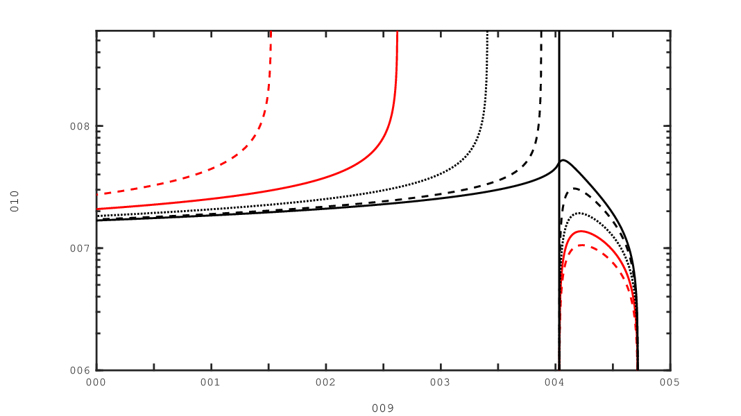
The turnover branch of the Alfvén mode for $z_{\rm A}>z_{\rm m}$ and $\rho\ll 1$ is dominated by the peak in $z^{2}W(z)$. For the case $\rho=1$ shown in Figure 7, the Alfvén mode consists of a thin loop, with the higher-frequency and lower-frequency portions joining at a turnover that corresponds to the peak at $z=z_{\rm m}$ in the RPDF. The maximum frequency of the Alfvén mode decreases with increasing $\theta$ approximately along the line $z=z_{\rm m}$. For $\rho\approx 1/\langle\gamma\rangle\ll 1$ the loop becomes narrower with decreasing $\rho$. The format adopted in Figures 6 and 7 makes it increasingly difficult to illustrate the dispersive properties due to the curves being strongly concentrated near $z=1$.

An alternative format is used in Figure 8 to show the dispersion curves near $z=1$: we plot $\omega/\omega_{\rm p}$ on a log scale as a function of $(1-z)/\rho^{2}$ for $\rho=0.1$, with $\beta_{\rm A}\approx 1.2\times 10^{2}$ and $\gamma_{\rm A}\approx 87$, and $0.01$, with $\beta_{\rm A}\approx 1.2\times 10^{3}$ and $\gamma_{\rm A}\approx 8.7\times 10^{2}$, where $\gamma_{\rm A}$ is defined by (47). The solid curves correspond to the L mode for $\theta=0$ and the solid vertical line is the dispersion curve $z=z_{\rm A}$ for the A mode. The curves to the left of $(1-z_{\rm A})/\rho^{2}$ correspond to the O mode and the curves to the right of $(1-z_{\rm A})/\rho^{2}$ correspond to the Alfvén mode. Each of $1-z_{\rm A}\approx 1/2\beta_{\rm A}^{2}$, $1-z_{\rm m}$ and $1-z_{0}$ is proportional to $\rho^{2}\approx 1/\langle\gamma\rangle^{2}$ as discussed in Section 3.3, so that the locations of the left asymptote, the peak and the right asymptote of the Alfvén mode all scale with $\rho^{2}$ and so coincide in the two Figures.

The Alfvén mode (for $\theta\neq 0$) exists only for $z<z_{\rm A}$ or $\gamma_{\phi}<\gamma_{\rm A}\approx\beta_{\rm A}$. Its dispersion relation, given by equation (26) with $a(z)>0$, becomes

The Alfvén mode is in the range where Landau damping is nonzero. Assuming that the waves are weakly damped only for $\gamma_{\phi}^{2}\gtrsim\gamma_{\rm m}^{2}$, the approximations $z_{\rm m}\approx 1-0.013\rho^{2}$, given by equation Table 1, and $\langle\gamma\rangle\approx 1/\rho$ imply that the waves are weakly damped for $\gamma_{\phi}\gtrsim 6\,\langle\gamma\rangle$.

The dispersion curves for parallel propagation, $\omega=\omega_{\rm L}(z)$ and $z=z_{\rm A}$, do not necessarily cross in a relativistic plasma. There are three possibilities:

• •

  $z_{\rm A}>z_{\rm m}$: the line $z=z_{\rm A}$ crosses the higher-frequency portion of the L mode dispersion curve $\omega=\omega_{\rm L}(z)$ in the range $1<z<z_{\rm m}$; reconnection in this case is similar to that in the cold-plasma limit. The peak in the dispersion curve is in the (reconnected) Alfvén mode.

• •

  $z_{\rm m}>z_{\rm A}>z_{0}$: the line $z=z_{\rm A}$ crosses the higher-frequency portion $\omega=\omega_{\rm L}(z)$ in the range $z_{\rm m}>z_{\rm A}>z_{0}$.

• •

  $z_{\rm A}<z_{0}$: the line $z=z_{\rm A}$ does not cross $\omega=\omega_{\rm L}(z)$.

Simple estimates for a pulsar magnetosphere suggest very large values, $\beta_{\rm A}\gg 1$, but before concentrating on this case we comment on the second and third cases.

References

- Arendt & Eilek (2002) Arendt, Jr., P. N. & Eilek, J. A. 2002 Pair Creation in the Pulsar Magnetosphere. Astrophys. J. 581, 451–469.
- Arons & Barnard (1986) Arons, J. & Barnard, J. J. 1986 Wave propagation in pulsar magnetospheres - Dispersion relations and normal modes of plasmas in superstrong magnetic fields. Astrophys. J. 302, 120–137.
- Asseo (1993) Asseo, E. 1993 Microtexture in the Pulsar Radio Emission Zone. Mon. Not. R. Astron. Soc. 264, 940.
- Asseo (1995) Asseo, E. 1995 The importance of boundary effects in the emission region of the pulsar magnetosphere. Mon. Not. R. Astron. Soc. 276, 74–102.
- Asseo & Melikidze (1998) Asseo, E. & Melikidze, G. I. 1998 Non-stationary pair plasma in a pulsar magnetosphere and the two-stream Instability. Mon. Not. R. Astron. Soc. 301, 59–71.
- Asseo et al. (1983) Asseo, E., Pellat, R. & Sol, H. 1983 Radiative or two-stream instability as a source for pulsar radio emission. Astrophys. J. 266, 201–214.
- Asseo & Riazuelo (2000) Asseo, E. & Riazuelo, A. 2000 Relativistic anisotropic pair plasmas. Mon. Not. R. Astron. Soc. 318, 983–1004.
- Benford & Buschauer (1977) Benford, G. & Buschauer, R. 1977 Coherent pulsar radio radiation by antenna mechanisms - General theory. Mon. Not. R. Astron. Soc. 179, 189–207.
- Beskin & Philippov (2012) Beskin, V. S. & Philippov, A. A. 2012 On the mean profiles of radio pulsars - I. Theory of propagation effects. Mon. Not. R. Astron. Soc. 425, 814–840.
- Egorenkov et al. (1983) Egorenkov, V. D., Lominadze, D. G. & Mamradze, P. G. 1983 Beam instability of the plasma in pulsar magnetospheres. Astrophysics 19, 426–431.
- Eilek & Hankins (2016) Eilek, J. A. & Hankins, T. H. 2016 Radio emission physics in the Crab pulsar. J. Plasma Phys. 82 (3), 635820302.
- Gallant et al. (1992) Gallant, Y. A., Hoshino, M., Langdon, A. B., Arons, J. & Max, C. E. 1992 Relativistic, perpendicular shocks in electron-positron plasmas. Astrophys. J. 391, 73–101.
- Gedalin et al. (2002) Gedalin, M., Gruman, E. & Melrose, D. B. 2002 New Mechanism of Pulsar Radio Emission. Phys. Rev. Lett. 88 (12), 121101.
- Godfrey et al. (1975) Godfrey, B. B., Newberger, B. S. & Taggart, K. A. 1975 A relativistic plasma dispersion function. IEEE Transactions on Plasma Science 3, 60–67.
- Hardee & Rose (1976) Hardee, P. E. & Rose, W. K. 1976 A mechanism for the production of pulsar radio radiation. Astrophys. J. 210, 533–538.
- Hardee & Rose (1978) Hardee, P. E. & Rose, W. K. 1978 Wave production in an ultrarelativistic electron-positron plasma. Astrophys. J. 219, 274–287.
- Hibschman & Arons (2001) Hibschman, J. A. & Arons, J. 2001 Pair Production Multiplicities in Rotation-powered Pulsars. Astrophys. J. 560, 871–884.
- Hinata (1976a) Hinata, S. 1976a Level of electrostatic excitation associated with relativistic beam-plasma system and pulsar radiation. Astrophys. Space Sci. 44, 389–395.
- Hinata (1976b) Hinata, S. 1976b Relativistic plasma turbulence and its application to pulsar phenomena. Astrophys. J. 206, 282–294.
- Iwamoto et al. (2017) Iwamoto, M., Amano, T., Hoshino, M. & Matsumoto, Y. 2017 Persistence of Precursor Waves in Two-dimensional Relativistic Shocks. Astrophys. J. 840, 52.
- Jüttner (1911) Jüttner, F. 1911 Das Maxwellsche Gesetz der Geschwindigkeitsverteilung in der Relativtheorie. Annalen der Physik 339, 856–882.
- Kaplan & Tsytovich (1973) Kaplan, S. A. & Tsytovich, V. N. 1973 Plasma astrophysics. Pergamon Press, Oxford.
- Lominadze & Mikhailovskiǐ (1979) Lominadze, D. G. & Mikhailovskiǐ, A. B. 1979 Longitudinal waves and two-stream instability in a relativistic plasma. Sov. Phys. JETP 49, 483.
- Lominadze et al. (1979) Lominadze, D. G., Mikhaǐlovskiǐ, A. B. & Sagdeev, R. Z. 1979 Langmuir turbulence of a relativistic plasma in a strong magnetic field. Sov. Phys. JETP 50, 927.
- Lominadze & Pataraya (1982) Lominadze, J. G. & Pataraya, A. D. 1982 Some nonlinear mechanisms of pulsar emission. Physica Scripta T2, 215–222.
- Lominadze et al. (1982) Lominadze, J. G., Stenflo, L., Tsytovich, V. N. & Wilhelmsson, H. 1982 A new explanation of the high effective temperatures in pulsar radioemissions. Physica Scripta 26, 455–458.
- Luo & Melrose (2004) Luo, Q. & Melrose, D. B. 2004 Orthogonal Mode Polarization of Pulsar Radio Emission. In Young Neutron Stars and Their Environments (ed. F. Camilo & B. M. Gaensler), IAU Symposium, vol. 218, p. 381.
- Luo et al. (2002) Luo, Q., Melrose, D. B. & Fussell, D. 2002 Wave dispersion in gyrotropic relativistic pulsar plasmas. Phys. Rev. E 66 (2), 026405.
- Lyubarskii (1992) Lyubarskii, Y. E. 1992 Possible mechanism of pulsar radio emission. Astron. Astrophys. 265, L33–L36.
- Lyutikov (1999) Lyutikov, M. 1999 Beam instabilities in a magnetized pair plasma. J. Plasma Phys. 62, 65–86.
- Lyutikov (2000) Lyutikov, M. 2000 Excitation of Alfvén waves and pulsar radio emission. Mon. Not. R. Astron. Soc. 315, 31–36.
- Medin & Lai (2010) Medin, Z. & Lai, D. 2010 Pair cascades in the magnetospheres of strongly magnetized neutron stars. Mon. Not. R. Astron. Soc. 406, 1379–1404.
- Melrose (1986) Melrose, D. B. 1986 Instabilities in Space and Laboratory Plasmas. Cambridge University Press.
- Melrose (2008) Melrose, D. B. 2008 Quantum Plasmadynamics: Unmagnetized Plasmas. New York: Springer.
- Melrose (2013) Melrose, D. B. 2013 Quantum Plasmadynamics: Magnetized Plasmas. New York: Springer.
- Melrose & Gedalin (1999) Melrose, D. B. & Gedalin, M. E. 1999 Relativistic Plasma Emission and Pulsar Radio Emission: A Critique. Astrophys. J. 521, 351–361.
- Melrose et al. (1999) Melrose, D. B., Gedalin, M. E., Kennett, M. P. & Fletcher, C. S. 1999 Dispersion in an intrinsically relativistic, one-dimensional, strongly magnetized pair plasma. J. Plasma Phys. 62, 233–248.
- Melrose & McPhedran (1991) Melrose, D. B. & McPhedran, R. C. 1991 Electromagnetic Processes in Dispersive Media. Cambridge University Press.
- Sironi & Spitkovsky (2009) Sironi, L. & Spitkovsky, A. 2009 Particle Acceleration in Relativistic Magnetized Collisionless Pair Shocks: Dependence of Shock Acceleration on Magnetic Obliquity. Astrophys. J. 698, 1523–1549.
- Stix (1962) Stix, T. H. 1962 The Theory of Plasma Waves. McGraw-Hill.
- Suvorov & Chugunov (1973) Suvorov, E. V. & Chugunov, Y. V. 1973 Distribution Function of Relativistic Electrons in a Strong Magnetic Field. Astrophys. Space Sci. 23, 189–199.
- Suvorov & Chugunov (1975) Suvorov, E. V. & Chugunov, Y. V. 1975 Electromagnetic waves in a relativistic plasma with a strong magnetic field. Astrophysics 11, 203–222.
- Synge (1957) Synge, J. L. 1957 The relativistic gas. Amsterdam : North-Holland Pub. Co, bibliography: p. [105].
- Timokhin & Arons (2013) Timokhin, A. N. & Arons, J. 2013 Current flow and pair creation at low altitude in rotation-powered pulsars’ force-free magnetospheres: space charge limited flow. Mon. Not. R. Astron. Soc. 429, 20–54.
- Tsytovich & Kaplan (1972) Tsytovich, V. N. & Kaplan, S. A. 1972 Relativistic turbulent plasma in pulsars. Astrofizika 8, 441–460.
- Ursov & Usov (1988) Ursov, V. N. & Usov, V. V. 1988 Plasma flow nonstationarity in pulsar magnetospheres and two-stream instability. Astrophys. Space Sci. 140, 325–336.
- Usov (1987) Usov, V. V. 1987 On two-stream instability in pulsar magnetospheres. Astrophys. J. 320, 333–335.
- Usov (2000) Usov, V. V. 2000 Radiating Regions in Pulsar Magnetospheres: From Theory to Observations and Back. In IAU Colloq. 177: Pulsar Astronomy - 2000 and Beyond (ed. M. Kramer, N. Wex & R. Wielebinski), Astronomical Society of the Pacific Conference Series, vol. 202, p. 417.
- Weatherall (1994) Weatherall, J. C. 1994 Streaming instability in relativistically hot pulsar magnetospheres. Astrophys. J. 428, 261–266.
- Weatherall (1997) Weatherall, J. C. 1997 Modulational Instability, Mode Conversion, and Radio Emission in the Magnetized Pair Plasma of Pulsars. Astrophys. J. 483, 402–413.
- Weatherall (1998) Weatherall, J. C. 1998 Pulsar Radio Emission by Conversion of Plasma Wave Turbulence: Nanosecond Time Structure. Astrophys. J. 506, 341–346.
- Wright & Hadley (1975) Wright, T. P. & Hadley, G. R. 1975 Relativistic distribution functions and applications to electron beams. Phys. Rev. A 12, 686–697.
Appendix A Dispersion equation
Here we present the derivation of nonzero components of , defined in (45), and discuss our assumptions.
A.1 Dielectric tensor
Consider a plasma that is composed of electrons, , and positrons, . The general form for the dielectric tensor derived using kinetic theory involves a sum over . For a 1D distribution it is convenient to replace the conventional distribution function, , and the integral over by the 1D distribution with , , , and the integral over . The dielectric tensor is given by (Melrose 2008; Melrose 2013)