The Supercooled Universe
Abstract
Strongly-coupled theories at the TeV can naturally drive a long period of supercooling in the early universe. Trapped into the deconfined phase, the universe could inflate and cool down till the temperature reaches the QCD strong scale. We show how at these low temperatures QCD effects are important and could trigger the exit from the long supercooling era. We also study the implications on relic abundances. In particular, the latent heat released at the end of supercooling could be the reason for the similarities between dark matter and baryon energy densities. The axion abundance could also be significantly affected, allowing for larger values of the axion decay constant. Finally, we discuss how a long supercooling epoch could lead to an enhanced gravitational wave signal.
1 Introduction
As the LHC continues exploring the TeV-scale territory, searching for hints on the origin of the electroweak (EW) scale, it is also quite necessary to look for probes of new physics in other environments, as for example in the early universe. This is of vital importance due specially to the LHC energy limitation, as these probes could indirectly provide evidences for new physics just beyond the LHC reach.
New strongly-interacting sectors at the TeV scale are particularly well-motivated examples for explaining the origin of the EW scale, and are at present exhaustively searched at the LHC. These models also present dark matter (DM) candidates that are searched for at present experiments. In spite of this, there is a generic prediction for these TeV strong sectors that has not been fully explored and can have a strong impact in the physics of the early universe: a long epoch of supercooling arising as a result of the transition from the deconfined to the confined phase. The main purpose of this article is to address under which conditions this long epoch of supercooling can happen, and explore the phenomenological consequences in the early universe.
The basic dynamics which gives birth to such a supercooled universe is the following. Strongly-interacting theories are expected to be in a deconfined phase at temperatures above the TeV, in which its constituents behave as a strongly-interacting hot gas. When the temperature goes down below the TeV, the confined phase becomes energetically favorable. Nevertheless, when the rank of the strong gauge group is large, the phase transition is of first-order and can only be completed through tunneling. Since the tunneling rate is quite suppressed , the transition cannot occur, and the universe enters a potentially eternal epoch of inflation trapped in the deconfined phase. As the temperature decreases, however, the QCD critical temperature is attained. Since these TeV strong sectors must be coupled to the SM quarks (to give them masses after the EW breaking), strong QCD effects become important at low temperatures and can be responsible for triggering the phase transition and ending the supercooling era. Therefore, a natural consequence of TeV-scale strong sectors is a long epoch of supercooling, which can last for several efolds.
The idea of a supercooled universe in which the phase transition is driven by QCD condensation was first considered in [1], in the context of the Coleman-Weinberg model, and has been also recently discussed in [2] in strongly-coupled models similar to the ones discussed here.11 1 Supercooling with holographic duals was first considered in [3]. Since then, several studies of the confinement phase transition have been performed with short periods of supercooling [4, 5, 6, 7, 8, 9, 10, 11, 12, 13]. Our first main goal in this article is to address the general conditions under which this long epoch occurs. We will define the essential ingredients of the strongly-coupled models needed for supercooling and exiting at temperatures around or below the QCD strong scale. As we will see, it will be crucial to distinguish between models in which the EW symmetry is restored in the deconfined phase from those in which it is broken. This latter possibility has not been considered before, and, as we will see, can lead to important implications for axion physics. We will also present holographic examples of these type of models that allow to calculate tunneling rates and determine the exit from supercooling.
Next, we will explore the consequences for cosmology. We will see that the release of entropy at the end of the phase transition leads to a strong dilution of DM relics. This implies a different range of couplings and masses for WIMP-like DM candidates and wimpzillas. Also for DM candidates that get their masses after the phase transition (e.g., resonances of the strong sector), we will see that their relic abundances are mainly determined by their initial thermal abundance and the dilution from supercooling. Interestingly, we will show that this can also be the case for the baryon asymmetry, and therefore the supercooled universe could give an explanation for the observed similarity between the baryon and DM energy density.
We will also study the implications for the QCD axion. We will see that during the supercooling epoch the axion could oscillate and quickly relax to the minimum of its potential. Therefore, its relic abundance could be reduced, meaning that larger values of the axion decay constant will be favored for axion DM. Whenever axionic topological defects are relevant, their contribution to the axion relic abundance can also be enhanced in the supercooled universe. This is essentially due to the fact that the inflationary expansion delays the collapse of the axionic string-wall network compared to the standard case.
Perhaps the most model-independent implication of a confinement phase transition is the gravitational wave (GW) signal. This has received a lot of attention in recent literature, but not for the particular case of long supercooling in which the thermal plasma which surrounds the colliding bubbles of the confined phase is very diluted. We will see that the GW signal after a long supercooling epoch can be sourced mostly by the collisions of bubbles of the confined phase, which occurs on a long time scale and thus maximizes the amplitude of the signal.
The organization of the paper is as follows. In Section 2 we introduce the properties of the strongly-coupled sectors in the confined phase and deconfined phase (Sec. 2.1). In Section 3 we analyze the deconfinement-confinement phase transition, calculating the tunneling rates and the temperature for exiting. In Section 4 we study the cosmological consequences of a long period of supercooling for dark matter (Sec. 4.1) and for baryons (Sec. 4.2). Axion dark matter from misalignment is discussed in Sec. 4.3.1, while the impact on axionic topological defects is given in Sec. 4.3.2. Gravitational wave signals are discussed in Sec. 4.4. Section 5 is devoted to conclusions. We add two appendices. In Appendix A we present holographic models with the same properties of the strongly-coupled sectors that lead to supercooling. In Appendix B we review some basics of axion DM from the string-wall network.
2 A strongly-interacting new sector at the TeV
We are interested in studying the supercooled phase of a strongly-interacting sector, or its equivalent five-dimensional version based on the AdS/CFT correspondence. We will identify here the generic properties (at zero ) of this class of theories relevant for our analysis:
- •
We assume that these are strongly-interacting conformal field theories (CFT) with a large central charge, or, equivalently, a large number of “colors” . This includes any gauge theory, e.g. , in the large limit.
- •
These CFTs will contain a small marginally relevant deformation that will be responsible for generating at the IR the confinement scale TeV, much smaller than any UV-scale, , as for example, the Planck-scale. This deformation can arise from a marginal operator added to the CFT, e.g.,
(2.1) where Dim with . The marginal coupling RG-evolves towards the IR until a critical value is reached at which conformal invariance is lost and a mass-gap is generated. In this class of theories, like in QCD, we expect a tower of resonances of different spin, weakly-coupled in the large limit, and with masses of order . This corresponds to the confined phase.
- •
As these models have usually accidental global symmetries, , an important parameter is the scale of spontaneous symmetry breaking (SSB) . We will refer to this scale as . This is associated to the nonzero condensate of an operator of the model transforming under . For example, in QCD this is supposed to be the quark condensate . We will assume, like in QCD or other gauge theories studied in the lattice, that (all condensates are of the same order). This is needed for phenomenological reasons, as the scale is associated with the electroweak scale that cannot be larger than the masses of the new resonances, bounded by the LHC to be above the TeV. For example, in composite Higgs models [14] where the Higgs is a PGB arising from the breaking , the Higgs VEV is given by where is an coefficient and . In fact, in many models a small tuning is required () to fulfill the experimental constraints [15].
- •
In order to study the phase transitions of the above models, it is crucial to understand these theories off-shell. This is a very difficult task, even for the holographic versions discussed in Appendix A. Nevertheless, this problem simplifies substantially whenever the lightest state is the dilaton, , the Goldstone parametrizing the spontaneous breaking of the scale invariance. In this case, we can study the effective potential of the dilaton after integrating out all other heavier states. We can understand this potential based on symmetries. Since under scale transformations, we have and , the effective potential can be written as
(2.2) where the dependence of the quartic coupling on is dictated by the explicit breaking of scale invariance. We identify with the minimum of the dilaton potential Eq. (2.2), . Notice that contrary to the Higgs and other fields, for the dilaton we will work in the basis in which its kinetic term is non-canonically normalized:
(2.3) where is a constant of and we are assuming that the dilaton is a glueball. This normalization guarantees and resonances get masses proportional to with no factors:
(2.4) where . In holographic models the dilaton is the radion and one obtains and (see Appendix A). The mass of the dilaton is given by
(2.5) where and . Notice that the dilaton effective potential makes sense for ; using Eq. (2.4), this gives the rough bound , where we have used holography in the last equality.22 2 It is instructive to derive the value of at the minimum by equating Eq. (2.2) to the QCD vacuum energy with GeV and . One obtains as expected since QCD has no light dilaton. We will assume here that Eq. (2.2) describes the vacuum of the theory with the dilaton being the lightest state.
- •
An important property of this class of models that will be very relevant for the impact in cosmology is how the condensate , that breaks , behaves for small (off-shell) values of the dilaton . We will consider two possibilities:
- I.
All condensates are proportional to . This implies in particular .
- II.
The condensate of is determined to be around , independently of . We have then even when .
It is important to understand the behavior of for the two types of models. In models of type I we expect to evolve logarithmically due to Eq. (2.1):
(2.6) where . At around crossing zero, develops a minimum à la Coleman-Weinberg. This is illustrated in Fig. 1. For constant we expect
(2.7) which for requires in order to generate TeV. Holographic weakly-coupled models with this property have been constructed, and are usually referred to as Goldberger-Wise models [16]. In these particular models can be computed and is a quadratic function of (see e.g. [3]).
On the other hand, models of type II correspond, for example, to models at which the dimension of the operator is not constant but, due to Eq. (2.1), RG-evolves till it becomes imaginary at some scale, signaling the breaking of the conformal symmetry with . They are referred to as walking models (see for example [17]) and the holographic versions correspond to 5D models with an AdS tachyon as described in Appendix A. For these type of models one finds that for the quartic goes as[18]
(2.8) with 1, and can have a minimum at some scale . For the quartic becomes almost constant (or at most evolving like Eq. (2.6)) as the theory can be described by another CFT (since part of the original CFT has become massive at ). This is shown in Fig. 1.
Figure 1: Behavior of the quartic coupling (upper plot) and effective potential for the dilaton (lower plot) as a function of for models of type I and type II . - I.
- •
Another relevant ingredient of this class of models is how they couple to the SM quarks. This coupling must be present, since we need the Higgs (coming from the new strong sector) to give mass to the SM quarks. The most realistic possibility is to have a linear coupling of the SM quarks to operators of the strong TeV sector:
(2.9) that is the portal of the SM quarks to the strong TeV sector, and therefore to the Higgs. Eq. (2.9) tells us that the composite operators must transform as a fundamental representation under QCD, that implies that there must be states charged under both the strong TeV sector and QCD. This requirement will have important implications when, in the supercooling phase, drops below the QCD confinement scale .
We can find weakly-coupled models with the properties described above by using the AdS/CFT correspondence (for models of type I, see [14], while for models of type II, see [18]). The importance of these toy models is that they allow to perform calculations and study the supercooling phenomena in a more quantitative way (for previous work, see [3, 4, 5, 6, 7, 8, 9, 10, 11, 12, 13]).
2.1 Deconfined phase
At high-temperatures a strongly-interacting theory is expected to have a different more energetically favorable phase in which the constituents are not confined into hadrons. In QCD this is the quark-gluon plasma phase. For the models described above we will assume that indeed this phase exists.
In this deconfined phase models of type I and II will have different properties. Models of type I are similar to QCD, in which all the condensates are zero and the theory has no mass gap in the deconfined phase. In particular, we expect that the Higgs does not get a VEV in this phase. On the other hand, in models of type II we have that independently of the scale of condensation , and therefore the electroweak symmetry is also broken in the deconfined phase, , for . We notice, as this will be important later when discussing axion physics, that is expected to be slightly larger than the Higgs VEV in the confined phase, 246 GeV, since to pass experimental constraints one needs TeV [15].
We will be interested later in studying the effects of QCD condensation in the CFT deconfined phase. For this reason, it is important to know what is the QCD scale in the deconfined phase . This scale is generically different from its value in the SM vacuum MeV as the CFT, which contains charged states under QCD, can contribute to the running of below the TeV scale. The equation that governs the running of at the one-loop level takes the well known form
| (2.10) |
where is the renormalization scale, while and are respectively the number of active flavors and colors. The contribution of the CFT is taken into account in the last term. Even though is not computable, holography tells unambiguously that it is positive, since corresponds to the inverse of the 5D gauge coupling squared in units of the AdS length [14]. By use of Eq. (2.10) we find that
| (2.11) |
where we normalized to the SM value. The parameter is given by
| (2.12) |
Eq. (2.11) is valid for . For the positive contributions to Eq. (2.10) win over the contributon of the gluons, and QCD is not confining, i.e., . Since the CFT always gives a positive contribution to the beta function, we have , 33 3 is negative because it is dominated by the contribution of the gluons. and as a consequence . Nevertheless, we can allow for the possibility that the QCD group arises as the low-energy remnant of a larger gauge group ( for simplicity), spontaneously broken by the strong dynamics of the CFT at the scale . In this case can be negative and then . 44 4 The possibility to have a larger QCD scale in the early universe by giving a VEV to a scalar coupled to has also been considered [19] (see also [20]). This could also be possible here. For example, for and , we get , giving .
3 Confined-deconfined phase transition and supercooling
If our universe was ever in the deconfined phase described in the previous section, it must have transitioned to the confined phase at some time during cosmic evolution. The temperature at which this becomes thermodynamically possible can be estimated as follows: in the unconfined phase the only relevant scale is temperature, and we then expect the free energy density to scale as in a hot free gas with d.o.f., that is . On the other hand, in the confined phase the CFT acquires a mass gap, , and at the heavy resonances are not excited (due to Boltzmann suppression). Therefore the free energy is dominated by the temperature-independent vacuum energy, . The phase transition can take place as soon as .
In large- gauge theories it is found that the confinement phase transition is of first order; this is also seen in holographic models in which the two phases correspond to two different solutions of the same Lagrangian (see Appendix A), and therefore one can only go from one to the other by bubble nucleation. It is thus crucial to compute , the rate at which bubbles are produced: in particular, the transition can be completed only when (see e.g. [21]) where is the Hubble constant that in the confined phase for is dominated by the vacuum energy:
| (3.1) |
where we have used Eq. (2.5) with and as we will take from now on. In a semi-classical approximation is given by
| (3.2) |
where is the action of the critical bubble, or bounce, and is typically of order , being the critical bubble radius. When the bounce is dominated by the dynamics of the large- sector, we have and is exponentially suppressed. If the transition cannot take place the universe inflates in the confined phase and exponentially cools down.
Before going into the details of the tunneling process, let us first compute more precisely the critical temperature below which confinement becomes favorable; for this we need to know the free energy in the two phases. As explained above, in the deconfined phase we can use conformal invariance and -counting to fix in the following way:
| (3.3) |
where is a constant of order 1; using holography we find , an larger than the free particle result (see Appendix A for a derivation). In the confined phase, for temperatures below , we have
| (3.4) |
where thermal corrections mainly come from light degrees of freedom (always present in realistic models). The critical temperature is given by equating in the two phases, which gives
| (3.5) |
where we normalize with the value coming from holography.
When the temperature of the universe goes below , bubbles of the confined phase begin to form. It is in general not an easy task to compute the rate since the bounce can depend on many fields. To simplify the analysis, one usually looks for a preferred tunneling direction in field space, in order to reduce it to a single-field problem. In the confined phase we already argued that the dilaton is the only relevant field if we consider it lighter than the other resonances. Nevertheless, it is not at all obvious what are the relevant field and potential in the deconfined phase, and how to properly connect the two phases. These points were first discussed by the authors of Ref. [3] in the context of the holographic 5D model. Here, we briefly rephrase their strategy in purely 4D terms. The key observation is that both phases become indistinguishable in the limit at which the conformal symmetry is recovered in both phases. In Fig. 2 we plot the potential along the path that connects in this way the deconfined phase (on the left side) to the confined phase (on the right side). In the confined phase the field variable is , with potential given in Eq. (2.2), while in the deconfined phase the proper variable is the local temperature of the plasma, . The free energy density of the CFT plasma as a function of (see left of Fig. 2) can be easily fixed, up to a constant factor, with elementary arguments from thermodynamics, and has the following expression:
| (3.6) |
where the constant is fixed in such a way that Eq. (3.6) matches with Eq. (3.3) for . This result is also derived in Appendix A using holography. To completely specify the system, we finally need to normalize the kinetic term for . Even though it is not clear how to do it, not even from the holographic perspective, we take this to be . We will see however that the parameter does not impact sensibly the calculation of .

At finite temperature bubble nucleation can be induced either thermally or quantum mechanically. Which process is more likely can be determined by comparing and : when (high temperature regime) thermal bubbles are preferred, while for bubble nucleation is mainly driven by quantum fluctuations. For the two phases have almost degenerate and the thin wall regime applies. Moreover, it can be seen that quantum bubbles are highly disfavoured so that tunneling is driven by thermal fluctuations. Nevertheless, as was shown in Ref. [3], the tunneling rate is too slow for the transition to be completed in this regime. As the plasma cools to the properties of the critical bubble become very different. Firstly, the energy difference between the two phases increases and thick wall bubbles become favoured. Secondly, especially in the regime of long supercooling which we are interested in, thermal bubbles production is either disfavoured or comparable to quantum induced one, as we checked also by numerically solving the bounce equations for the two cases. Thus in the following we will focus on quantum tunneling in the thick wall regime.
From Fig. 2 we see that for lower and lower temperatures, the thermal barrier becomes smaller and smaller. In this regime it is not obvious where the field prefers to tunnel: whether it nucleates close to the minimum TeV or just beyond the barrier (that is, roughly, at ) depends on the fine details of the potential . The task of finding the tunneling point (see Fig. 2), as long as the bounce action , can be tackled by means of a thick wall approximation for [6] that, for a canonically normalized field , reads as
| (3.7) |
where is the position of the false vacuum and the minimization is over the tunneling point . In our specific case, Eq. (3.7) gives
| (3.8) |
where the prefactor comes from the non-canonical normalization of . We have checked that this formula is in good agreement with the numerical results obtained by solving the bounce equation in the limit .
Let us now work out the consequences of Eq. (3.8) for the models described in Sec. 2.
- •
Type I Models: In this case is given by Eq. (2.6), that can be conveniently rewritten as . In the limit , which is a consequence of , Eq. (3.8) can be solved, giving and 55 5 We notice that the terms proportional to in Eq. (3.8) give subleading contributions for .
(3.9) The bubble radius is roughly , so the prefactor is estimated as and the condition for exiting inflation gives
(3.10) The temperature at which the above condition is satisfied gives the exit temperature , which can be conveniently traded for the number of efolds of inflation as follows
(3.11) When the argument of the square root in Eq. (3.11) is negative, there is no solution to Eq. (3.10), meaning that the universe gets trapped in the deconfined phase. This occurs whenever
(3.12) where we normalized according to the discussion after Eq. (2.7). We see that exiting supercooling in these type of models is in tension with having a small , which is required to generate the hierarchy between and . We could imagine more favorable situations with not being constant, for example being small at the UV but rapidly growing towards (the range of which is important for discussing supercooling). This would allow to exit supercooling for larger values of , as appreciated in Fig. 3 where we show for different values of and . Nevertheless, having small (a long period of supercooling) seems to require precise values of and , which makes this quite unlikely.

Figure 3: Lines of fixed exit temperature ( GeV from below to above) for type I models, and no exit region Eq. (3.12). - •
Type II Models: These models have a larger (for TeV), which leads to faster tunneling rates. Using Eq. (2.8) with , we find that exit from supercooling roughly happens for When the parameters allow this, inflation ends for not far from . It is difficult to achieve small values of since becomes almost constant for small , as it is shown in Fig. 1. In other words, we find once more that long periods of supercooling are not expected.
The above conclusions can change drastically when drops close to . As we will see in the next section, at that scale QCD confines and can drive the supercooling era to an end.
3.1 Impact of QCD at low
If the universe is trapped in the CFT deconfined phase, the temperature will drop exponentially till reaching the QCD strong scale, where QCD effects could potentially become important. The relevance for supercooling of QCD condensates was first discussed in Ref. [1] in the context of the Coleman-Weinberg model (for recent studies see [22, 23, 24, 25]). Nevertheless, there is an important difference with the models discussed here. The Coleman-Weinberg is a weakly-coupled model where the scalar (which can be considered a dilaton with a potential as Eq. (2.2)) is an elementary particle. For this reason a huge fine-tuning is required to put to zero the mass term that, on general grounds, could be present. The models discussed here however are strongly-coupled theories in which the dilaton is composite and therefore the potential Eq. (2.2) arises naturally without fine-tuning.
The first analysis of the impact of QCD in models of composite dilatons was done in Ref. [2]. The authors study the contributions of the QCD vacuum energy to the dilaton potential. This is estimated to be
| (3.13) |
where can be extracted from QCD data (taking and MeV), and is the QCD strong scale as a function of . This dependence on the value of arises, as explained in Sec. 2.1, from the CFT states charged under QCD that affect the running of from high-energies down to . Indeed, using Eq. (2.10), it can be shown that
| (3.14) |
where is given in Eq. (2.12). For , Eq. (3.13) can become larger than at small . For example, at , where is maximized, this happens for
| (3.15) |
If this is the case, Eq. (3.13) dominates the dilaton potential and the tunneling rate can be estimated as 66 6 This is is obtained by solving Eq. (3.8) with Eq. (3.13), taking into account that in the deconfined phase there is also the contribution . The tunneling point is of order and the bubble size .
| (3.16) |
and the condition for exiting supercooling at being . Since Eq. (3.16) scales as , exit from supercooling is only possible for small values of . In particular, we find for and . For a more detailed exploration see however Ref. [2].
3.1.1 Fate of the new strong sector for below
As goes below , we expect the impact of QCD in the tunneling rate to be more dramatic, as the CFT can be drastically affected. Since some of the CFT constituents are charged under color, we expect them to take mass at and decouple at around this scale, analogously to hadrons in the SM below the GeV. We cannot really compute what is the fate of the CFT at smaller scales, but it is not unconceivable that, after this drastic departure from near-conformality, the theory flows into another (quasi) CFT. An example of this behavior is provided by QCD in the conformal window, where the theory can remain conformal even after integrating out some flavors. If this is the case, we can parametrize this effect as a drastic change of the quartic coupling at , as well as a change in its beta-function, . Taking and as free parameters, the tunneling rate will be given by
| (3.17) |
valid under the conditions that and (which are also the conditions that favor tunneling for ). Notice that, contrary to Eq. (3.16), the bounce action is not enhanced by , which makes the supercooling exit much more probable. In Fig. 4 we plot the contours of fixed , the efolds of inflation after the QCD phase transition is crossed, in the parameter space of and , where we have taken .
We conclude that under reasonable assumption on the strongly-coupled CFT the universe could be trapped in the unconfined phase till it reaches . At this temperature, or slightly below (see Fig. 4), the tunneling rate to the CFT confined phase can be large enough due to QCD, leading to the end of this long supercooling epoch.
4 Cosmological Implications
How would we know if the universe indeed experienced such a long supercooling epoch? The purpose of this section is to describe observational consequences of the associated long period of vacuum domination, which would provide evidence for this phenomenon (see also [4, 5, 6, 7, 8, 9, 10, 11, 12, 26, 27, 28, 13, 29, 30, 31, 32] for related analyses but where mainly only short eras of supercooling were considered).
Let us start with the universe at high-temperatures, reheated after a first epoch of inflation, responsible for the generation of the CMB anisotropies. As the temperature cools down and reaches , the universe gets trapped in the CFT deconfined phase, and a second inflationary epoch begins with Hubble rate given by Eq. (3.1). Following the discussion in Sec. 3.1, we will mainly consider that the exit from supercooling occurs at or slightly after QCD confinement, i.e. after efolds.77 7 The duration of supercooling is in principle not strongly constrained by CMB anisotropies, because density and/or isocurvature fluctuations are not abundantly produced [33]. At the end of the supercooling era, there is an injection of entropy due to the first-order phase transition. While reheating (RH) in this case can be in general a complicated process, the natural expectation is that most of the energy available in the deconfined phase is transferred to radiation in the confined phase. This leads to
| (4.1) |
where we have used Eq. (3.3) with . Here is the number of relativistic species after reheating. Thus the entropy injection after supercooling is given by
| (4.2) |
where and are respectively the entropy density at reheating and ; the latter can be read from Eq. (3.6) evaluated at . This release of entropy strongly dilutes the abundances of constituents which exist in the deconfined phase. This is in particular the case for particles heavier than the TeV scale as well as for baryons, as we will discuss in Sec. 4.1 and Sec. 4.2 respectively. The same conclusion applies to quanta of a QCD axion field, if the latter oscillates during supercooling (see Sec. 4.3.1). However, the relevance of axionic topological defects is generically enhanced in the supercooled universe, as we will discuss in Sec. 4.3.2.
At the end of the first order phase transition, reheating occurs via violent processes, which source gravitational radiation. While this implication has already been thoroughly discussed in the literature (see refs. above), our long epoch of inflation can lead to a maximal signal, dominantly due to the collision of bubbles of the confined phase, as we will discuss in Sec. 4.4.
4.1 Dark Matter abundance
Let us start with the implications for dark matter (DM) particles. In the strongly-interacting scenarios considered above, we can consider two classes of dark matter candidates (apart from the QCD axion that will be discussed in the next section): those which are heavy in both CFT phases, or, alternatively, those which are massive in the confined phase but massless in the deconfined phase, i.e., . In both cases, supercooling affects the relic abundance only if the dark matter is not repopulated after reheating. If a generic DM particle has mass and annihilation cross section in the confined phase, its thermal production after supercooling is subdominant whenever , where is the freeze-out temperature of . For , one finds . Therefore, according to Eq. (4.1), thermal production after supercooling can be neglected when . In what follows we will focus on this case.88 8 Non-thermal production after supercooling can also be relevant in principle. Indeed, in a first-order phase transition with runaway bubbles, the possibility exists to abundantly produce heavy dark matter particles during the bubble collisions [9, 34, 35]. This occurs only when collisions are approximately elastic. However, in our case the two minima of the dilaton potential are highly non-degenerate, which implies that bubble collisions are likely quite inelastic. This remains true even if the field tunnels to a value of the potential which is close to the false minimum, since it rolls down the true minimum before the bubbles have time to meet. Therefore non-thermal production of heavy dark matter from bubble collisions is suppressed in our scenarios.
Let us consider first the dilution of DM candidates that are massive in both phases, , and whose thermal freeze-out temperature is above . Their relic abundance today can be computed starting from the number density-to-entropy ratio . After freeze-out, is constant, except at the phase transition where the entropy changes according to Eq. (4.2). Therefore, the relic abundance of is given by
| (4.3) |
In the second line of Eq. (4.1) we have assumed and normalized to the SM QCD critical temperature. Eq. (4.1) is simply the standard relic abundance of a WIMP-like particle with a very small prefactor due to supercooling. If we assume and , Eq. (4.1) implies for 100 MeV.99 9 Heavy particles which interact with nuclei can be looked for at DM direct detection experiments. Interestingly, if , the region of parameter space suggested by Eq. (4.1) is currently probed by XENON1T [36] and will be further investigated by LZ [37]. If we assume instead , Eq. (4.1) matches the observed DM abundance for GeV. Thus in the supercooled universe wimpzillas do not need to be very weakly coupled in order not to overproduce dark matter.
Let us now move to species which are massless in the deconfined phase and massive in the confined phase, . We only demand these states to be stable. Their relic abundance can be computed again from , which in the deconfined phase is given by , with the entropy given in Eq. (3.6). The number density of today can be thus simply obtained by dividing by Eq. (4.2) and multiplying by the entropy density today. The relic abundance of is thus given by
| (4.4) |
where is an efficiency prefactor which takes into account the possibility that is further diluted as its mass switches on during the phase transition. If the DM is a composite state in the confined phase, Eq. (4.4) should include a further prefactor to take into account the decrease of degrees of freedom in DM from the deconfined to the confined phase. From Eq. (4.4) we can conclude that a TeV-scale particle can reproduce the observed dark matter abundance if supercooling lasts approximately until the temperature of the SM QCD phase transition (see [38] for similar conclusions).
4.2 Coincidence between baryon and dark matter abundances
Similarly as dark matter, any baryon asymmetry generated at high temperature will be diluted by the inflationary expansion during supercooling. This opens the possibility to explain the smallness of by the dilution factor Eq. (4.2). Furthermore, if both dark matter and baryons arise from relativistic particles that were in thermal equilibrium at some , their abundances will be comparable before supercooling and equally diluted at the end of the phase transition. This could then provide an explanation for the coincidence of DM and baryon abundances, with their energy density ratio mainly determined by the ratio of their masses.
As an illustrative example of the above idea, let us consider the case in which a (B-L) asymmetry is generated at temperatures above , from the out-of-equilibrium decay of a very heavy state (generic in UV completions which include gravity). For , is in thermal equilibrium, thus its number density is comparable to the rest of the thermal bath, i.e. . Once , the inverse decays are Boltzmann-suppressed and a baryon asymmetry can be generated if the out-of-equilibrium condition is fulfilled. If this is the case, we expect , where is the CP asymmetry in the decay of to (B-L)-charged particles. After supercooling, the baryon number is diluted in the same way as in the case of DM. Following the same steps which lead to Eq. (4.4), we can estimate the baryon-to-entropy ratio to be
| (4.5) |
If and , the observed baryon asymmetry can be obtained for . As the origin of Eq. (4.5) is similar to DM in Eq. (4.4), we can easily estimate the ratio of baryon to DM energy density to be
| (4.6) |
where is the proton mass and we have also included a possible dilution factor for , as in Eq. (4.4). It is quite interesting that the ratio of baryon and DM relic abundances is predicted to be very simply related to the ratio of their masses and of the efficiencies of CP violation and DM number changing processes at the end of the phase transition. In order to obtain the observed value , Eq. (4.6) leaves two options:
-
with . However, in this case one needs to make sure that the DM is not copiously produced at reheating and that its supercooling abundance is not overcome by later thermal or sub-thermal production. As explained above, this forces us to consider , which might be challenging to achieve.
-
with . This implies that the DM abundance has to be further diluted during the phase transition. This is not inconceivable: in the case of the electroweak phase transition it is indeed known that at the bubble walls, particles can undergo transition radiation and lose energy via the emission of massive particles [39]. While we do expect the same phenomenon to occur in the deconfined-confined transition, we are not currently aware of quantitative estimates.
In the light of the arguments presented in this subsection, it would be extremely interesting to understand whether a low reheating temperature and/or small can be obtained in the supercooling setup. We leave this task for future work.
4.3 The QCD axion
Let us now discuss the implications of supercooling for the QCD axion. In the deconfined phase SM quarks can be either massless or massive, depending on whether the Higgs VEV (or that of the equivalent operator ) is zero or not in this phase. On one hand, in models of type I, all VEVs are zero in the deconfined phase and quarks are then massless. In this case the axion mass is quite small in the deconfined phase1010 10 Even for , the axion mass is not zero since there is still a very small Higgs-mediated contribution. and supercooling does not alter the relic abundance from the misalignment mechanism (see [40] for previous studies). On the other hand, in models of type II, we have TeV and the SM quarks are instead massive in the deconfined phase. Axion oscillations can then take place during the supercooling inflationary expansion as well as , where is the axion mass in the deconfined phase. In this case the axion field can rapidly relax to the minimum and its relic abundance from the misalignment mechanism can be diluted, as we will explain in detail below. Axionic topological defects can instead be affected by supercooling in both type of models, as it will be discussed at the end of this section.
The standard axion cosmology begins when the PQ symmetry is broken at , where is the axion decay constant. Below this temperature, the axion dynamics is dictated by the Klein-Gordon equation
| (4.7) |
The potential is periodic and negligible at high temperatures, while it rises very rapidly around the QCD phase transition:
| (4.8) |
with and (see [41] for an analytic determination and [42] for lattice confirmation). Below , the axion mass is given by
| (4.9) |
According to Eq. (4.7), axion oscillations start at determined by , i.e. at GeV for standard axion parameters. Below axion quanta behave as DM, according to the misalignment mechanism. The QCD axion relic abundance depends on whether the PQ symmetry is broken during or after cosmological inflation. In the latter case, the initial average value of the axion field is and axion oscillations generate the observed dark matter abundance for . If instead the PQ symmetry is broken during inflation, larger values of are phenomenologically viable if is appropriately tuned.
4.3.1 Supercooling and the misalignment mechanism
Let us now investigate the effects of supercooling on the misalignment mechanism. We approximate Eq. (4.8) with the quadratic expansion around the minimum, since the effect of anharmonicities is not especially relevant for our estimates. The value of the axion field at the end of the supercooling era depends on the axion mass Eq. (4.9) with , the Hubble scale Eq. (3.1), and the number of efolds of supercooling. In particular, Eq. (4.7) admits three regimes for the amplitude of the axion field:
| (4.10) | ||||
| (4.11) | ||||
| (4.12) |
The underdamped case corresponds to the well-known dark matter behavior , with a prefactor due to the temperature dependence of . The condition provides an upper bound on :
| (4.13) |
The implication of Eq. (4.13) is as follows: On one hand, if is smaller than Eq. (4.13), then the axion oscillates during the supercooling epoch and relaxes to the minimum if . On the other hand, if is much larger than Eq. (4.13), the axion is slowly-rolling along its potential: according to Eq. (4.12), it relaxes to the minimum only for .
The observationally allowed value of depend on the duration of supercooling. In Fig. 5 we provide two examples of constraints on and from the overproduction of axion DM. We use TeV and fix 1111 11 See [43] for constraints on the dilaton mass from collider searches., () in the left (right) plot in Fig. 5. The dilution of the axion field does not depend on the initial value of the axion but to fix ideas we have taken as in the post-inflationary axion scenario. The dashed orange lines in the plots correspond to exiting at the QCD critical temperature, . Assuming that the exit from supercooling occurs after the QCD phase transition, the upper bound on can be pushed slightly above for . For , slightly above is allowed. The available parameter space is reduced as decreases and/or increases, as dictated by Eq. (4.13). In particular for the axion field is essentially frozen during the supercooling epoch and the standard computation of the axion relic abundance is not significantly altered. We also show in Fig. 5 regions of parameter space where the QCD axion represents only a fraction of the DM. These are relevant for axion DM detection experiments (e.g. ADMX [44]), which are sensitive to .

A few comments are in order. One can argue that the constraints on can also be relaxed in the standard case by demanding that the PQ symmetry is broken during inflation, as this allows to tune the initial condition to any desired value. The mechanism presented here, however, provides a dynamical way to implement this initial condition, without appealing to any anthropic tuning.1212 12 See [45, 46] for an alternative possibility in the framework of low-scale models of eternal inflation. Furthermore, our setup can still preserve the predictivity of the standard post-inflationary axion scenario. Indeed, the inflationary expansion during supercooling is too short to homogenize the axion field across the Hubble volume today, thus in our case one still has to average over randomly distributed axion values.
4.3.2 Supercooling and axionic topological defects
In the previous subsection we have focused on the relic abundance from the misalignment mechanism. However, further contributions to the axion energy density can arise from topological defects (see [47] for an excellent introduction). We now study how the latter are affected by supercooling. The standard lore is that inflationary expansion strongly dilutes pre-existing topological defects. However, we will argue here that if the PQ symmetry is broken after cosmological inflation, supercooling generically enhances the relevance of axionic strings and domain walls.
The history of axionic topological defects starts at , when the Peccei-Quinn symmetry is broken and string-like defects form. They evolve until in a radiation dominated background, according to the so-called scaling behavior: at any given cosmological time there is approximately one horizon-length string per Hubble volume (for a recent analysis, see [48, 49, 50]). This fast dilution is partially due to the emission of massless axion quanta from to . The relic number density of such axions is dominated by particles emitted at .
In the standard cosmological history, the axion potential Eq. (4.8) switches on at the QCD phase transition and domain walls form, which are attached to the strings. Such walls pull the strings together and thus destroy the network if (see [51, 48]). In the supercooling scenario strings are pushed beyond the cosmological horizon by the inflationary expansion. At the QCD phase transition during supercooling, strings are not in causal contact and the network cannot annihilate, since two strings cannot feel the attractive force of the wall stretching between them. Therefore, the network survives the first QCD phase transition.
After reheating, as drops in the ordinary expanding universe, the string network re-enters the comoving Hubble sphere at the temperature . There are now two possible scenarios depending on :
-
: the standard cosmology of topological defects and their contribution to axion dark matter is not significantly affected.
-
: in this case strings re-enter the horizon when . Therefore, the string-wall network is immediately formed and rapidly decays. The contribution to the axion dark matter abundance is given by (see Appendix B for a derivation)
(4.14) Constraints on and from dark matter overproduction are shown in Fig. 6. We are neglecting the contribution coming from the misalignment mechanism. This is justified for the relevant range of and (see Fig. 5). The effect of supercooling is essentially to delay the collapse of the string-wall network, which leads to stronger bounds on . En passant, let us notice that such a delayed annihilation of axionic topological defects could lead to the formation of Primordial Black Holes [52].
Figure 6: Constraints on and from DM overproduction from the late decay of the axionic string-wall network. The solid blue line is obtained imposing , according to Eq. (4.14). The orange region is forbidden by astrophysical observations. The solid green line represent the critical temperature of the ordinary QCD phase transition after reheating. The dashed lines show the corresponding number of efolds of supercooling.
4.4 Gravitational waves
The exit from the supercooling era occurs via a strong first order phase transition and thus generates gravitational radiation. Differently from other scenarios discussed in the literature, we focus here on the case in which the phase transition takes place after a long inflationary phase. As we will discuss, this implies that the gravitational wave signal is dominantly due to the collision of bubbles of the confined phase. A further peculiarity of our setup is the possibility to obtain the maximal strength of the signal, because of a long duration of the phase transition.
The gravitational wave signal depends mainly on two parameters: the duration of the phase transition, usually denoted with , and the latent heat released during the phase transition. The former can be computed starting from the time variation of the nucleation rate, i.e. (see e.g. [53]) and for the case of supercooling is given by [54]
| (4.15) |
Here we denote with and the Hubble rate during supercooling Eq. (3.1) and at the reheating temperature respectively. For fast reheating they are expected to be similar, . The latent heat is instead given by [54]
| (4.16) |
In our setup , while can vary between and . As we will see below, the strength of the gravitational wave signal is maximized for and .
Until recently, it was thought that if a first order phase transition occurs during vacuum domination, bubbles of true vacuum would reach a runaway regime (see e.g. [54]). This means that bubbles are accelerated until they actually collide, such that most of the energy available in the phase transition is deposited in the accelerating walls. If this is the case and bubbles expand at speeds very close to luminal, then a naive estimate of the wall -factor at the time of collision is , where is the initial bubble radius at . This gives
| (4.17) |
for the values of which we find in our models. The subsequent collisions of several bubbles generate a strong gravitational wave signal, whose spectrum is given by [54] 1313 13 After publication of this work, we became aware of analytical studies of the gravitational wave signal from bubble collisions [55, 56], which also go beyond some of the approximations assumed in Eq. (4.4). For runaway bubbles, such as the ones we consider here, the gravitational wave spectrum at small frequencies turns out to scale as , while the peak frequency is slightly smaller than (4.19).
| (4.18) |
where is the bubble wall velocity, is the fraction of the latent heat which goes into kinetic energy of the bubble walls and is the frequency, whose value at the peak of the signal is given by
| (4.19) |
This simple picture has been recently challenged in [39], where it is shown that in a first-order EWPT bubbles surrounded by a radiation bath tend instead to reach a limit -factor, even when the plasma is significantly diluted. This is due to transition radiation of particles in the bath: as they cross the wall, they can emit vector bosons whose mass changes across the wall. This phenomenon translates into the following friction pressure
| (4.20) |
where is the electroweak coupling and is the typical difference in masses across the wall. In a first-order EWPT this is . As the bubble expand, increases till it reaches a critical value, , at which balances the energy difference between the true and false vacua, and the bubble velocity becomes constant. For a first-order EWPT with , one finds .
Now, whenever , the bubble can reach -factors of order before they collide. If this is the case (as for example for the first-order EWPT), most of the energy available in the phase transition will be released to the surrounding plasma. Since this latter also sources gravitational radiation, either from sound waves or turbulence effects, the gravitational wave signal will be significantly changed (see e.g. [54]).
The confinement phase transition studied in this paper is different from a first-order EWPT studied in [39]. In particular, the plasma surrounding the bubbles is strongly interacting in our case. Nevertheless, we can expect that transition radiation could also occur here. If we assume that Eq. (4.20) approximately holds in our case, we can estimate
| (4.21) |
which is larger than for MeV, indicating that cannot be achieved for these small values of . As we have seen in the previous section, in the long supercooling scenarios considered here, we can easily achieve MeV (see for example Fig. 4). If this is the case, bubbles would be effectively in the runaway regime until collision. We can then envision the following options for the gravitational wave signal in our scenarios:
-
: bubbles expand and reach , giving a gravitational wave signal dominantly sourced by the plasma which surrounds the bubbles. The amplitude and spectrum of this type of signals were analyzed in [54], but this may not straightforwardly extend to our case where is very large. Nevertheless, in the cases which are currently understood, the slope of the spectrum is larger than in Eq. (4.4), the amplitude is linear in and for it is of the same order of magnitude as Eq. (4.4).
-
: in this case it is reasonable to assume that bubbles effectively run away and the effects of the plasma can be neglected. The gravitational wave signal is given by Eq. (4.4) and depends only on for large . As a concrete example, let us consider the exit induced by QCD with given by Eq. (3.17). In this case, we have , according to Eq. (4.15). Thus, having leads to . Very interestingly, we therefore find that whenever the friction of the plasma can be neglected by exiting from supercooling at sufficiently low temperatures, the duration of the phase transition is very long and the GW signal is maximized. This conclusion is not significantly affected by the exact value of and . This is true also for , as long as .1414 14 If and exit occurs due to QCD, then friction can always be neglected, independently from the value of .
In Fig. 7 we show two representative gravitational wave spectra, obtained by fixing and for simplicity. We vary instead the exit temperature . We see that a very strong signal can indeed be obtained if exit occurs much below (blue curve): the peak amplitude is close to the upper bound from dark radiation at BBN [57] and the signal is detectable at the least sensitive configuration of the LISA interferometer, possibly even at the ET. A weaker signal (orange line), which is nevertheless detectable at more sensitive configurations of LISA, is instead obtained if the exit occurs closer to . Both signals are significantly larger than the more commonly considered case . However, we stress that a detailed analysis of the thermal friction in the confinement phase transition is required to more confidently assess the shape and size of the GW spectrum in our case.

5 Conclusions
We have studied the conditions for having a long period of supercooling driven by strongly-coupled theories at the TeV, which arises due to the small tunneling rate of the confinement phase transition. We have calculated these rates for several examples, and showed that quite generically (for reasonable values of and the dilaton mass) the universe gets trapped in the deconfined phase, starting a new period of inflation. As the supercooled universe expands and cools down, the temperature reaches the QCD strong scale, , where QCD effects become relevant. We have shown that these effects can be calculated for but are suppressed by . For the CFT drastically changes as QCD-color states get massive and decouple from the rest of the CFT, affecting the tunneling rate by effects. Under some reasonable assumptions we have shown that these can lead to an end of supercooling after efoldings.
We have also studied the cosmological consequences of a long period of supercooling. Very generically, at the end of supercooling any DM candidate is diluted by Eq. (4.2). Under the assumption that DM is not reheated again after the phase transition, we have seen that WIMP-like DM candidates need to have very different properties. In particular, see 4.1, their masses can be as large as GeV for generic DM couplings of order for 100 MeV. For DM candidates that get masses from the TeV strong scale , and are massless in the deconfined phase, their relic abundances are mainly determined by their thermal number density at and the dilution factor Eq. (4.2), as shown in Eq. (4.4). This can also be the case for baryons, as we have seen in the particular case in which the baryon asymmetry is generated from decaying particles that were in thermal equilibrium at high temperatures. This provides an interesting explanation for having a ratio of baryon to DM energy densities roughly proportional to the ratio of their masses, even though the mechanisms that originate them were very different.
One of the main impact of a long supercooling epoch is for the QCD axion abundance. We find that during supercooling we can have (not possible for inflation at higher energies), implying that the axion can oscillate towards its minimum. This is possible in models in which the EW symmetry is broken in the deconfined phase. This leads to an extra dilution of axions as compared to the standard case, which changes the predictions for being DM. We find that larger values of are required (see Fig. 5), weakening the signal in experiments searching for DM axions such as ADMX [44]. On the other hand, the contributions from axionic topological defects can be enhanced in a supercooled universe. This is because, due to the inflationary expansion, the axionic string-wall network can collapse later than in the standard cosmology. Therefore, the network can provide a larger contribution to the axion relic abundance, which would limit the allowed values of , see Fig. 6.
Finally, we have also explored the GW signal arising from the end of the supercooling epoch. We identified two peculiarities of our setup, which can simplify the estimates of the GW spectrum, as well as maximize the signal. Firstly, due to the long inflationary expansion, the plasma which surrounds the bubble can be severely diluted: this implies and that the friction on the bubble motion can be likely neglected. Therefore, bubble collisions can be effectively considered as the main source of gravitational radiation. Secondly, due to the very same reason, one can have , which leads to a stronger GW signal than in the usual case, see Fig. 7.
There are many things left for future work. It would be very useful to better understand how the CFT behaves at in order to get a better prediction for . For DM candidates we have seen that the reheating process at the end of the phase transition deserves more attention as it is crucial to determine their abundances. Also it is important to understand transition radiation effects in the confinement phase transition as this plays a crucial role in the GW signal.
Acknowledgments
We thank J. Garriga., B. von Harling, A. Katz, O. Pujolàs and G. Servant for discussions. A.P. has been supported by the Catalan ICREA Academia Program. This work has also been partly supported by the grants FPA2014-55613-P, FPA2017-88915-P, 2017-SGR-1069 and SEV-2016-0588.
Appendix A Holography and Supercooling
Using the AdS/CFT dictionary [58, 59], we can identify weakly-coupled five-dimensional models with the same properties of the strongly-coupled theories described in Section 2. This provides us with simple calculable models to address the supercooling phenomena in a more quantitative way. Many examples were considered before in the literature [3, 4, 5, 6, 7, 8, 9, 10, 11, 12, 13]. Here we briefly recall the entries of the dictionary that are useful for studying our problem.
The “dual” five-dimensional models are characterized by an AdS5 geometry:
| (A.1) |
solution to the 5D Einstein equations for metric with negative cosmological constant
| (A.2) |
where is the AdS curvature radius, the 5D Planck mass and the 5D Ricci scalar. This five-dimensional space is assumed to be ending by a hard-wall, often called IR-brane, at some position in the extra dimension, . For Eq. (A.1) to actually be a solution ending with a hard-wall at , the hard-wall must have a negative tension . When this condition is met the value of is not dynamically fixed but free to take any value. In fact spans a moduli space of equivalently solutions to Eq. (A.2). The AdS/CFT dictionary tells that the radion corresponds to the dilaton of the CFT model via the identification . The tuning of the IR-brane tension to the value above corresponds to tune the dilaton potential to zero.
The moduli space parametrized by is actually part of a larger manifold of solutions, parametrized by itself and a four dimensional constant matrix , generalizing the matrix in Eq. (A.1). This moduli space is associated to massless fields in 4D, corresponding to the spacetime dependent fluctuations of the moduli “coordinates” (or ) and . When rewriting the Einstein 5D action Eq. (A.2) in terms of the moduli fields, we get the 4D action
| (A.3) |
where is the 4D Ricci scalar constructed from . The AdS/CFT correspondence relates the 5D Planck mass in units of to the rank of the 4D gauge group , according to . The dilaton is not canonically normalized, and Eq. (A.3) fixes the coefficient of Eq. (2.3) to . The massive Kaluza-Klein modes are interpreted in the 4D as resonances of the strongly coupled CFT, and their masses are given by
| (A.4) |
corresponding to fix in Eq. (2.4).
In the 5D models discussed here we also need the equivalent of the 4D marginally relevant operator Eq. (2.1) with . By use of the AdS/CFT dictionary, we know that operators in the CFT are mapped to 5D fields in AdS with the same quantum numbers. Also the dimensions of the 4D scalar operators are related to the masses of the 5D fields according to
| (A.5) |
where is the mass of . Therefore, the marginally relevant operator Eq. (2.1) is associated to an almost massless scalar in the five-dimensional theory, . Furthermore, we have the mapping , that triggers a nonzero profile for in the bulk.
Let us now move to the symmetry breaking pattern. The AdS/CFT dictionary tells that having the global symmetries in the CFT corresponds to gauging a group in the 5D bulk, and the SSB by a scalar condensate translates to having an extra 5D scalar in the bulk, , transforming under , that gets an nonzero VEV on the IR-brane. The SM Higgs is associated to be one of the zero-modes of after KK-reduction.
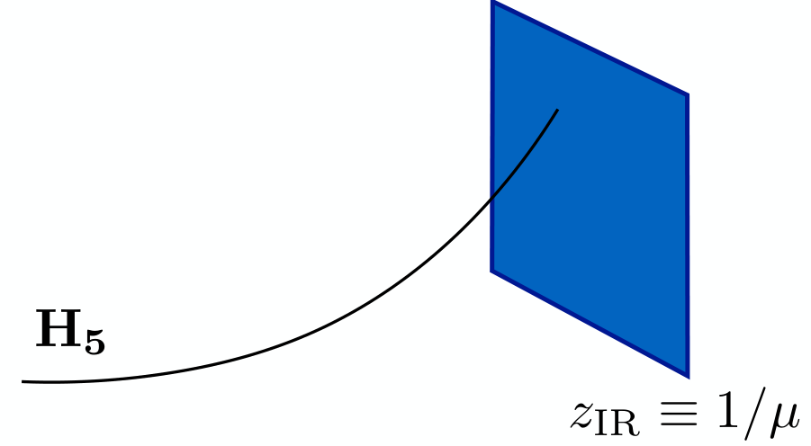
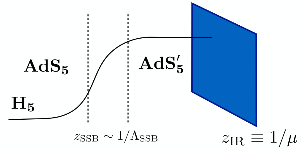
In realistic models the potential of the radion/dilaton should not be fixed to zero but be generated from the 5D model in order to naturally make . Let us qualitatively discuss how this can arise in the 5D versions of models of type I and II studied in the paper:
- I.
In this case the radion/dilaton potential arises from the almost massless field , as in Goldberger-Wise models [16]. has a potential on the IR-brane that gives a non-zero VEV for at the IR-brane. We have in this case that the VEV profile of is peaked towards the IR-brane and therefore . This possibility is illustrated by the left figure of Fig. 8.
- II.
is coupled to that gives him a -dependent mass, . At some , we have that becomes smaller than the BF-bound (), and becomes an AdS5 tachyon. In this case gets a nonzero profile in the 5D bulk that grows as , till reaches the minimum of its 5D potential and becomes constant in . The value of where the maximum is achieved, , is associated with the SSB scale . When including the metric back-reaction, one gets that the AdS5 geometry evolves at around into another AdS5 with different curvature. The dual 4D interpretation of this is that a CFT RG-evolves into another CFT at . The tachyon profile gives also a contribution to the radion potential and a minimum for can be achieved, as studied in Ref. [inpreparation]. One usually finds . When moving the IR-brane off-shell towards the horizon , the VEV of is not proportional to and then does not go to zero as in type I models. This is illustrated in the right figure of Fig. 8.
Let us finally provide the 5D implementation of Eq. (2.9). The fermionic operators corresponds to 5D fermions with the same quantum numbers as the SM quarks. This implies that the QCD group must be a gauged symmetry in the 5D bulk. At low energies, the zero-modes of these 5D fermions corresponds to the SM quarks.
A.1 The deconfined phase
In 5D holographic versions the deconfined phase is characterized by a different solution to the 5D Einstein equations (arising from Eq. (A.2)) at finite temperature where we must take the Euclidian version of the theory, with compact time . This solution is called AdS5-Schwarzschild Black Hole (AdS-BH) geometry, and the metric can be expressed as
| (A.6) |
This metric has a BH horizon at replacing the infrared brane ( runs from to ). The BH horizon is associated to a Hawking temperature, given by . To avoid singularities, we must match the BH Hawking temperature with the temperature of the system: (see A.2 for more details).
On the AdS-BH background Eq. (A.6) the 5D fields which were discussed above, and in particular , take in general a different profile. We are especially interested in the value of in models I and II . In type I models cannot get a nonzero profile in the AdS-BH solution since, contrary to the IR-brane, there is no potential for in the BH solution. On the other hand, in models of type II , is an AdS5 tachyon and then also turns on even in the absence of an IR-brane potential. Indeed, we can find a nonzero profile for in the AdS-BH where at the regularity of the solution implies
| (A.7) |
Therefore, the EW symmetry is broken in type II models also in the deconfined phase.
A.2 Free energy of the deconfined phase
The energy of solution Eq. (A.6) is interpreted in the 4D as the free energy of the plasma phase, with identification . In fact, when the metric Eq. (A.6) has a conical singularity at that gives a finite contribution to the free energy density equal to [3]
| (A.8) |
We see that it correctly vanishes when . A remaining piece comes from the regular region . This is UV divergent, but what matters for tunneling is its finite difference with the energy of full AdS5. This gives
| (A.9) |
When added together, the two contributions Eq. (A.8) and Eq. (A.9) give
| (A.10) |
where the last equality comes from the identification . With this identification we get for Eq. (3.3). The minimum of Eq. (A.10) is attained when , as it must be since Einstein equations forbid conical singularities.
This result can also be determined, modulo an overall constant, from elementary thermodynamics and scale invariance as follows. If we put a small region of volume to temperature , its free energy density (with respect to a thermal bath at temperature ) will be . The total energy and entropy and are extensive variables, and scale invariance tells that the densities and are appropriate powers of the only available scale (that is respectively and )
| (A.11) |
We know that is a minimum at thermal equilibrium, that is when . This fixes the ratio universally for any CFT.
Appendix B Axion dark matter from string-wall network
The aim of this appendix is to review the estimate of the contribution to the total axion dark matter abundance from the annihilation of the string-wall network (see e.g. [51]). The energy of the network is dominated by the walls, thus we have
| (B.1) |
where is the wall tension. This energy is eventually entirely released in axion quanta which behave like dark matter. The process is expected to occur very quickly after . The relic number density of the radiated particles is thus given by
| (B.2) |
where is the mean energy of the radiated axions at . This has to be extracted from numerical simulations: here we follow the results of [51], according to which . The relic energy density of such axions is given by
| (B.3) |
Finally the relic abundance is
| (B.4) |
References
- [1] E. Witten, Cosmological Consequences of a Light Higgs Boson, Nucl. Phys. B177 (1981) 477–488.
- [2] B. von Harling and G. Servant, QCD-induced Electroweak Phase Transition, JHEP 01 (2018) 159, [arXiv:1711.11554].
- [3] P. Creminelli, A. Nicolis, and R. Rattazzi, Holography and the electroweak phase transition, JHEP 03 (2002) 051, [hep-th/0107141].
- [4] L. Randall and G. Servant, Gravitational waves from warped spacetime, JHEP 05 (2007) 054, [hep-ph/0607158].
- [5] J. Kaplan, P. C. Schuster, and N. Toro, Avoiding an Empty Universe in RS I Models and Large-N Gauge Theories, hep-ph/0609012.
- [6] G. Nardini, M. Quiros, and A. Wulzer, A Confining Strong First-Order Electroweak Phase Transition, JHEP 09 (2007) 077, [arXiv:0706.3388].
- [7] B. Hassanain, J. March-Russell, and M. Schvellinger, Warped Deformed Throats have Faster (Electroweak) Phase Transitions, JHEP 10 (2007) 089, [arXiv:0708.2060].
- [8] T. Konstandin, G. Nardini, and M. Quiros, Gravitational Backreaction Effects on the Holographic Phase Transition, Phys. Rev. D82 (2010) 083513, [arXiv:1007.1468].
- [9] T. Konstandin and G. Servant, Natural Cold Baryogenesis from Strongly Interacting Electroweak Symmetry Breaking, JCAP 1107 (2011) 024, [arXiv:1104.4793].
- [10] T. Konstandin and G. Servant, Cosmological Consequences of Nearly Conformal Dynamics at the TeV scale, JCAP 1112 (2011) 009, [arXiv:1104.4791].
- [11] D. Bunk, J. Hubisz, and B. Jain, A Perturbative RS I Cosmological Phase Transition, Eur. Phys. J. C78 (2018), no. 1 78, [arXiv:1705.00001].
- [12] B. M. Dillon, B. K. El-Menoufi, S. J. Huber, and J. P. Manuel, Rapid holographic phase transition with brane-localized curvature, Phys. Rev. D98 (2018), no. 8 086005, [arXiv:1708.02953].
- [13] E. Megías, G. Nardini, and M. Quirós, Cosmological Phase Transitions in Warped Space: Gravitational Waves and Collider Signatures, JHEP 09 (2018) 095, [arXiv:1806.04877].
- [14] K. Agashe, R. Contino, and A. Pomarol, The Minimal composite Higgs model, Nucl. Phys. B719 (2005) 165–187, [hep-ph/0412089].
- [15] G. Panico and A. Wulzer, The Composite Nambu-Goldstone Higgs, Lect. Notes Phys. 913 (2016) pp.1–316, [arXiv:1506.01961].
- [16] W. D. Goldberger and M. B. Wise, Modulus stabilization with bulk fields, Phys. Rev. Lett. 83 (1999) 4922–4925, [hep-ph/9907447].
- [17] V. Gorbenko, S. Rychkov, and B. Zan, Walking, Weak first-order transitions, and Complex CFTs, JHEP 10 (2018) 108, [arXiv:1807.11512].
- [18] A. Pomarol, O. Pujolas and L. Salas, Holographic conformal transition and light scalars, [arXiv:1905.02653]
- [19] G. R. Dvali, Removing the cosmological bound on the axion scale, hep-ph/9505253.
- [20] S. Ipek and T. M. P. Tait, An Early Cosmological Period of QCD Confinement, arXiv:1811.00559.
- [21] D. S. Gorbunov and V. A. Rubakov, Introduction to the theory of the early universe, vol. I and II. 2011.
- [22] S. Iso, P. D. Serpico and K. Shimada, QCD-Electroweak First-Order Phase Transition in a Supercooled Universe, Phys. Rev. Lett. 119 (2017) no. 14 141301 [arXiv:1704.04955].
- [23] S. Arunasalam, A. Kobakhidze, C. Lagger, S. Liang and A. Zhou, Low temperature electroweak phase transition in the Standard Model with hidden scale invariance, Phys. Lett. B 776 (2018) 48, [arXiv:1709.10322].
- [24] Y. Bai and A. J. Long, Six Flavor Quark Matter, JHEP 1806 (2018) 072, [arXiv:1804.10249].
- [25] C. Marzo, L. Marzola and V. Vaskonen, Phase transition and vacuum stability in the classically conformal B-L model, [arXiv:1811.11169]
- [26] A. Kobakhidze, C. Lagger, A. Manning and J. Yue, Gravitational waves from a supercooled electroweak phase transition and their detection with pulsar timing arrays, Eur. Phys. J. C 77 (2017) no. 8, 570, [arXiv:1703.06552].
- [27] S. Bruggisser, B. Von Harling, O. Matsedonskyi, and G. Servant, Baryon Asymmetry from a Composite Higgs Boson, Phys. Rev. Lett. 121 (2018), no. 13 131801, [arXiv:1803.08546].
- [28] S. Bruggisser, B. Von Harling, O. Matsedonskyi, and G. Servant, Electroweak Phase Transition and Baryogenesis in Composite Higgs Models, Phys. Rev. Lett. 121 (2018) 131801, [arXiv:1804.07314].
- [29] I. Baldes and C. Garcia-Cely, Strong gravitational radiation from a simple dark matter model, arXiv:1809.01198.
- [30] J. Ellis, M. Lewicki, and J. M. No, On the Maximal Strength of a First-Order Electroweak Phase Transition and its Gravitational Wave Signal, arXiv:1809.08242.
- [31] T. Prokopec, J. Rezacek, and B. Świeżewska, Gravitational waves from conformal symmetry breaking, arXiv:1809.11129.
- [32] K. Miura, H. Ohki, S. Otani, and K. Yamawaki, Gravitational Waves from Walking Technicolor, arXiv:1811.05670.
- [33] M. S. Turner, E. J. Weinberg, and L. M. Widrow, Bubble nucleation in first order inflation and other cosmological phase transitions, Phys. Rev. D46 (1992) 2384–2403.
- [34] A. Falkowski and J. M. No, Non-thermal Dark Matter Production from the Electroweak Phase Transition: Multi-TeV WIMPs and ’Baby-Zillas’, JHEP 02 (2013) 034, [arXiv:1211.5615].
- [35] A. Katz and A. Riotto, Baryogenesis and Gravitational Waves from Runaway Bubble Collisions, JCAP 1611 (2016), no. 11 011, [arXiv:1608.00583].
- [36] XENON Collaboration, E. Aprile et al., Dark Matter Search Results from a One Ton-Year Exposure of XENON1T, Phys. Rev. Lett. 121 (2018), no. 11 111302, [arXiv:1805.12562].
- [37] B. J. Mount et al., LUX-ZEPLIN (LZ) Technical Design Report, arXiv:1703.09144.
- [38] T. Hambye, A. Strumia, and D. Teresi, Super-cool Dark Matter, JHEP 08 (2018) 188, [arXiv:1805.01473].
- [39] D. Bodeker and G. D. Moore, Electroweak Bubble Wall Speed Limit, JCAP 1705 (2017), no. 05 025, [arXiv:1703.08215].
- [40] G. Servant, Baryogenesis from Strong CP Violation and the QCD Axion, Phys. Rev. Lett. 113 (2014) no. 17 171803, [arXiv:1407.0030].
- [41] D. J. Gross, R. D. Pisarski, and L. G. Yaffe, QCD and Instantons at Finite Temperature, Rev. Mod. Phys. 53 (1981) 43.
- [42] S. Borsanyi et al., Calculation of the axion mass based on high-temperature lattice quantum chromodynamics, Nature 539 (2016), no. 7627 69–71, [arXiv:1606.07494].
- [43] K. Blum, M. Cliche, C. Csaki, and S. J. Lee, WIMP Dark Matter through the Dilaton Portal, JHEP 03 (2015) 099, [arXiv:1410.1873].
- [44] ADMX Collaboration, N. Du et al., A Search for Invisible Axion Dark Matter with the Axion Dark Matter Experiment, Phys. Rev. Lett. 120 (2018), no. 15 151301, [arXiv:1804.05750].
- [45] P. W. Graham and A. Scherlis, Stochastic axion scenario, Phys. Rev. D98 (2018), no. 3 035017, [arXiv:1805.07362].
- [46] F. Takahashi, W. Yin, and A. H. Guth, QCD axion window and low-scale inflation, Phys. Rev. D98 (2018), no. 1 015042, [arXiv:1805.08763].
- [47] A. Vilenkin and E. P. S. Shellard, Cosmic Strings and Other Topological Defects. Cambridge University Press, 2000.
- [48] V. B. Klaer and G. D. Moore, The dark-matter axion mass, JCAP 1711 (2017), no. 11 049, [arXiv:1708.07521].
- [49] M. Gorghetto, E. Hardy, and G. Villadoro, Axions from Strings: the Attractive Solution, JHEP 07 (2018) 151, [arXiv:1806.04677].
- [50] M. Kawasaki, T. Sekiguchi, M. Yamaguchi, and J. Yokoyama, Long-term dynamics of cosmological axion strings, arXiv:1806.05566.
- [51] M. Kawasaki, K. Saikawa, and T. Sekiguchi, Axion dark matter from topological defects, Phys. Rev. D91 (2015), no. 6 065014, [arXiv:1412.0789].
- [52] F. Ferrer, E. Masso, G. Panico, O. Pujolas, and F. Rompineve, Primordial Black Holes from the QCD axion, arXiv:1807.01707.
- [53] R. Apreda, M. Maggiore, A. Nicolis, and A. Riotto, Gravitational waves from electroweak phase transitions, Nucl. Phys. B631 (2002) 342–368, [gr-qc/0107033].
- [54] C. Caprini et al., Science with the space-based interferometer eLISA. II: Gravitational waves from cosmological phase transitions, JCAP 1604 (2016), no. 04 001, [arXiv:1512.06239].
- [55] R. Jinno and M. Takimoto, Gravitational waves from bubble collisions: An analytic derivation, Phys. Rev. D 95 (2017) no.2, 024009 [arXiv:1605.01403].
- [56] R. Jinno and M. Takimoto, Gravitational waves from bubble dynamics: Beyond the Envelope, JCAP 1901 (2019) 060 [arXiv:1707.03111].
- [57] C. Caprini and D. G. Figueroa, Cosmological Backgrounds of Gravitational Waves, Class. Quant. Grav. 35 (2018), no. 16 163001, [arXiv:1801.04268].
- [58] J. M. Maldacena, The Large N limit of superconformal field theories and supergravity, Int. J. Theor. Phys. 38 (1999) 1113–1133, [hep-th/9711200]. [Adv. Theor. Math. Phys.2,231(1998)].
- [59] E. Witten, Anti-de Sitter space and holography, Adv. Theor. Math. Phys. 2 (1998) 253–291, [hep-th/9802150].