Hydrodynamic interactions dominate the structure of active swimmers’ pair distribution functions
Abstract
Microswimmers often exhibit surprising patterns due to the nonequilibrium nature of their dynamics. Collectively, suspensions of microswimmers appear as a liquid whose properties set it apart from its passive counterpart. To understand the impact of hydrodynamic interactions on the basic statistical features of a microswimmer’s liquid, we investigate its structure by means of the pair distribution function. We perform particle-based simulations of microswimmers that include steric effects, shape anisotropy, and hydrodynamic interactions. We find that hydrodynamic interactions considerably alter the orientation-dependent pair distribution function compared to purely excluded-volume models like active Brownian particles, and generally decrease the structure of the liquid. Depletion regions are dominant at lower filling fractions, while at larger filling fraction the microswimmer liquid develops a stronger first shell of neighbors in specific directions, while losing structure at larger distances. Our work is a first step towards a statistico-mechanical treatment of the structure of microswimmer suspensions.
I Introduction
Collections of microorganisms such as bacteria or microalgae show a myriad of self-organized structures and patterns that are also governed by physical processes stemming from their nonequilibrium nature and mutual interactions. Some examples are self-concentration Schwarzendahl and Mazza 2018; Dombrowski et al. 2004, complex interaction with solid surfaces Ostapenko et al. 2018; Lauga et al. 2006; Berke et al. 2008, bacterial turbulence Wensink et al. 2012, swarming Copeland and Weibel 2009, spontaneous formation of spiral vortices Wioland et al. 2013, and directed motion Wioland, Lushi, and Goldstein 2016. Many of these systems collectively resemble the behavior and structure of a fluid and therefore it has been found useful to model these collections of organisms as an active or living fluid Koch and Subramanian 2011; Marchetti et al. 2013. Furthermore, the methods of statistical mechanics of classical fluids have been found to be powerful tools also in nonequilibrium situations, such as the analysis of velocity correlations and energy spectra for mesoscale turbulence of bacteria Wensink et al. 2012, and even a local equilibrium Maxwell–Boltzmann approximation for sedimenting active colloids Enculescu and Stark 2011.
The structure of an equilibrium fluid is typically analyzed in terms of the pair distribution function Allen and Tildesley 1989; Gray and Gubbins 1984, and is a cornerstone of liquid state theory Hansen and McDonald 1990. For active fluids, some work on the structural properties in terms of pair distribution functions has been put forward Bialké, Löwen, and Speck 2013; Härtel, Richard, and Speck 2018; Hoell, Löwen, and Menzel 2018; Wittkowski, Stenhammar, and Cates 2017; Riedel, Kruse, and Howard 2005; Alarcón and Pagonabarraga 2013; Kogler and Klapp 2015; Yang et al. 2017; Pessot, Löwen, and Menzel 2018; Locatelli et al. 2015; Theers et al. 2018; de Macedo Biniossek et al. 2018; Pessot, Löwen, and Menzel 2018. An important finding is the anisotropic form of the pair correlation function of active Brownian particles (ABP) presented in Bialké, Löwen, and Speck 2013; Härtel, Richard, and Speck 2018; Hoell, Löwen, and Menzel 2018; Wittkowski, Stenhammar, and Cates 2017, which arises from their self-propulsion.
Typically, pair correlation functions are strongly influenced by the mutual interactions between particles, which for microswimmers such as bacteria or algae moving in an aqueous milieu include hydrodynamic interactions. In this work we analyze the influence of the hydrodynamic interactions on the orientation-dependent pair distribution function of active swimmers, by considering a recent model for biological swimmers which also includes shape anisotropy and steric effects Schwarzendahl and Mazza 2018. In order to disentangle the effects of activity, hydrodynamic and steric interactions, we compare the pair distribution functions for our model to the case of active Brownian particles. We find that hydrodynamic interactions introduce considerably more structure to the pair distribution function at low filling fractions and suppress structures at high filling fractions.
The rest of this work is organized as follows. Section II introduces our model and the setup of the numerical simulations. In Sec. III we discuss the orientation-dependent pair distribution function, and its angular average: the radial distribution function. Section IV presents the distribution functions for both our swimmer’s model and for ABP. Finally, in Sec. V we collect our conclusions.
II Models and parameters
II.1 Stroke-averaged biological microswimmer

We employ the stroke-averaged biological microswimmer model presented in Schwarzendahl and Mazza 2018, which consists of an asymmetric dumbbell. Figure 1(a) shows a schematic representation of the puller-type model swimmer mimicking a Chlamydomonas reinhardtii cell, while Fig. 1(b) shows a schematic of the pusher-type model swimmer representing an Escherichia coli cell. In both cases, the small green sphere, marked with (1), represents the swimmer body and the large sphere, marked with (2), represents the stroke-average region spanned by the flagellar motion. The rigid motion of the dumbbells is governed by Newton’s equations and implemented via quaternion dynamics (for details see Schwarzendahl and Mazza 2018).
As hydrodynamic interactions between microswimmers can play an important role in their collective behavior, we also include an explicit model for the surrounding fluid by means of the multiparticle collision dynamics (MPCD) technique. MPCD is a particle-based method that reproduces hydrodynamic modes up to the Navier–Stokes level of description Gompper et al. 2009.
Experimental measurements Drescher et al. 2011 have shown that the flow field of the pusher-type swimmer can be modeled by a force dipole, whereas puller-type swimmers’ flow fields are well described by a combination of three-Stokeslets Drescher et al. 2010. We use regularized force regions, as shown by the red spheres with embedded arrows (3) in Fig. 1, to account for the hydrodynamic flow fields. Additionally, the dumbbells are coupled to the fluid by using a no-slip boundary condition on their surface (for more details see Schwarzendahl and Mazza 2018).
The temperature of the fluid, the size of an MPCD grid cell , and the mass of an MPCD particle , are the reference values for temperature, length, and mass, respectively. We perform simulations in a cubic domain of size with periodic boundary conditions in all three directions; each MPCD cell contains an average of MPCD particles, giving a total of MPCD particles in the system. The effective radius of an individual swimmer is . For further details on the numerical implementation the reader is referred to Schwarzendahl and Mazza 2018.
II.2 Active Brownian particles
In addition to the our stroke-averaged biological microswimmer, we also carry out simulations of ABP, to disentangle the effects of activity, hydrodynamic and steric interactions. ABP are spherical particles with radius that self-propel along their orientation with a typical speed (see also Wysocki, Winkler, and Gompper 2014; Fily and Marchetti 2012; Redner, Hagan, and Baskaran 2013; Bialké, Speck, and Löwen 2012). The translational motion of the particle’s position is governed by the equation
| (1) |
where the force between the particles is purely steric and is calculated from a Weeks–Chandler–Anderson potential Weeks, Chandler, and Andersen 1971. Here, is a Gaussian white noise with zero mean and , where is the translational diffusion coefficient. The motion of the orientational degrees of freedom is determined by the equation
| (2) |
where rotational diffusion is included by the Gaussian white noise with and the rotational diffusion coefficient is given by . Also for the ABP model, we use a three dimensional cubic domain with periodic boundary conditions.
II.3 Dimensionless parameters
For both our stroke-averaged biological microswimmer and ABP we simulate active swimmers, resulting in filling fractions from to , at a fixed volume . A dimensionless quantification of the relative importance of the self-propulsion speed to diffusive processes is the Péclet number, which we define as , where and are the effective speed and the effective size of the swimmer, respectively, and the diffusion constant of the swimmer (for ABP .) We present results at and . The Reynolds number of the flow around our swimmers (measuring the ratio of inertial to viscous forces) is given by , where and are the MPCD fluid’s density and viscosity, respectively. The simulated Reynolds numbers are for high Péclet number () and at lower Péclet number ().
III Pair distribution function
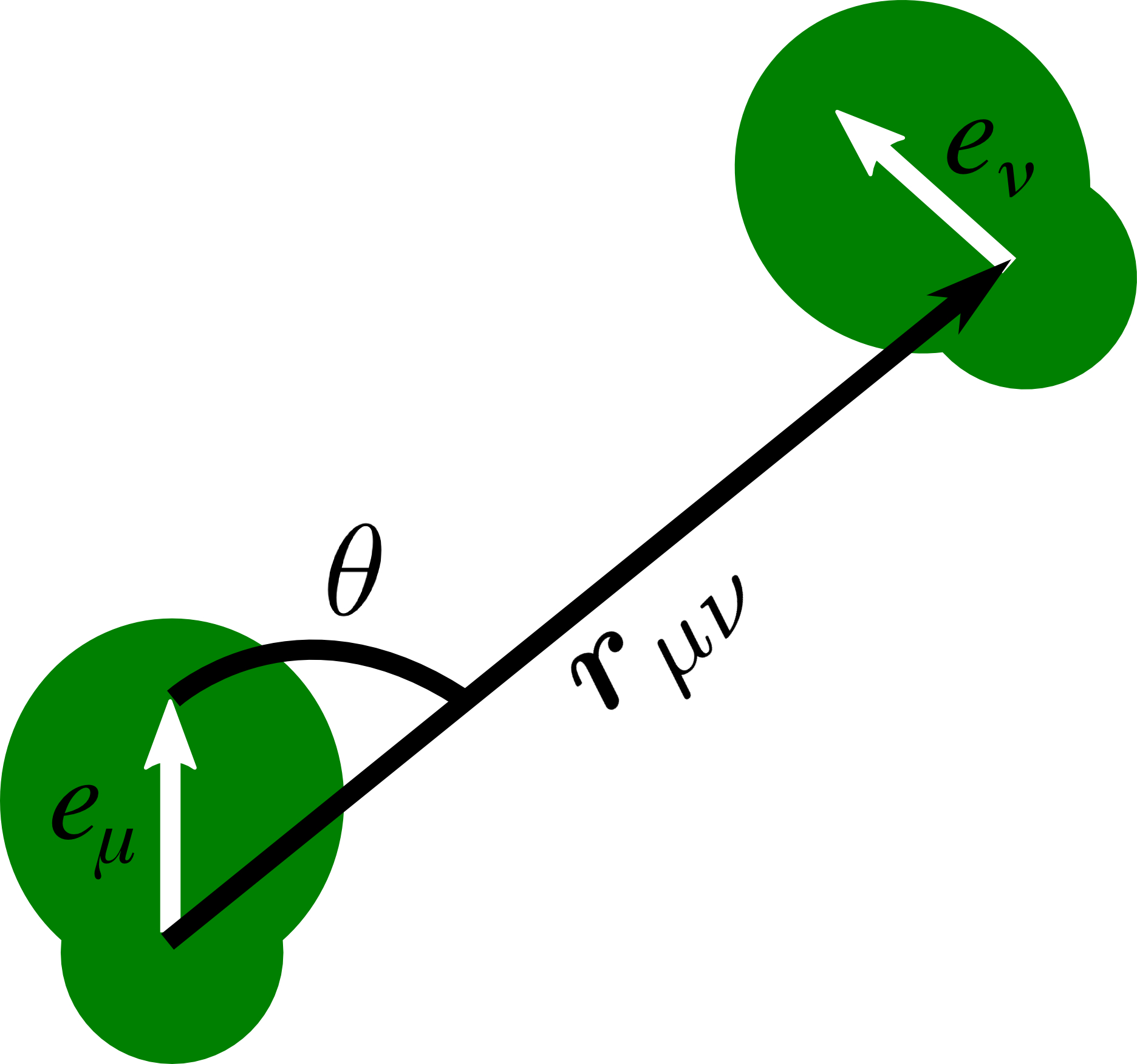
In general, the complete information of a liquid’s structure is encapsulated in the angular pair distribution function of two particles and , which depends on their relative position as well as on their orientations , Gray and Gubbins 1984; Allen and Tildesley 1989. However, in the general case the arguments of the pair distribution function are high dimensional and it has thus been proven useful to restrict oneself to a partial descriptions of the orientational ordering Allen and Tildesley 1989; Gray and Gubbins 1984. Since our active swimmers self-propel into the direction of their orientation , we are expecting non-trivial correlations mainly with respect to this axis. Therefore, we compute correlation of a particles orientation with respect to the relative position of all other particles, as illustrated in Fig. 2.
In practice, we use the following definition of our orientation-dependent pair distribution function: given two particles and with relative position and orientations , , we compute the distance and the polar angle with respect to the orientation of particle (Fig. 2). The average over the ensemble, polar angle, and orientation of the neighboring swimmer is obtained from a histogram for all pairs of swimmers, with radial bins and polar bins . The orientation-dependent pair distribution function is then given by
| (3) |
where is the normalization
| (4) |
where is the bin size in the radial component and is the bin size in the polar component. It should be noted that for a homogeneous configuration is equal to one. Physically, is related to the probability of finding a neighboring particle at distance and with a polar angle with respect to the reference particle and its orientation.
In addition to the orientation-dependent pair distribution function we calculate the radial distribution function Allen and Tildesley 1989; Hansen and McDonald 1990 given by
| (5) |
Furthermore, as an effective measure of the local structure around a microswimmer, we consider the coordination number Hansen and McDonald 1990, which is the average number of nearest neighbours of a particle
| (6) |
where is the position of the first minimum of .


IV Results
Figure 3 shows a matrix chart of our calculations of [Eq. (3)]. Different rows represent different Péclet numbers for both puller- and pusher-type swimmers, whereas the filling fraction changes with the column. First of all, low filling fractions are characterized by a complex texture of peaks and minima of . These are stationary state structures, and not transient, as explicitly verified in our simulations.
Pushers have increased probability to find neighbors in the frontal and rear polar regions of their bodies, while around their equator neighboring swimmers tend to be depleted. As the Péclet number increases, the asymmetry between front and back poles increases, and the rear tail region grows more populated than the front. Pullers present the most complex texture at low filling fractions. A preference for an accumulation of probability in the front pole and in the rear region at intermediate latitudes is, however, discernible. Furthermore, at low filling fraction, for both pullers and pushers shows a rather long-ranged structure, extending more than 5 times the radius of the individual swimmer.
As the filling fraction increases, loses structure for both pushers and pullers at all Péclet numbers. For pushers, perpendicular to the swimming direction the pair distribution function first increases to and then decreases to values . Furthermore, on the sides of the pushers one observes a band like structure for and a quadrupolar structure for . The increased values of in front and back poles of pushers become more concentrated in smaller areas as the filling fraction is increased.
For pullers, we observe that as increases, exhibits a ring-like structure of increased probability close to the swimmers. Furthermore, we find two distinct regions at intermediate latitudes in the rear region of the swimmer, within the ring-like structure, that show very large values of .
To disentangle the effects of activity, steric and hydrodynamic interactions on the pair distribution function, we performed additional simulations of ABP Wysocki, Winkler, and Gompper 2014; Fily and Marchetti 2012; Redner, Hagan, and Baskaran 2013; Bialké, Speck, and Löwen 2012, which only include steric interactions among swimmers. Figure 4 shows the orientation-dependent pair distribution function of ABP at different Péclet numbers and filling fractions. Even from a cursory inspection it is visible that the complex texture present at lower has nearly vanished. In its stead, a partial ring (interrupted in the lower pole) of pronounced peak of emerges. A clear increase to in front and a clear decrease to to behind the active Brownian particle can be seen. This asymmetry is an effect of the self-propulsion of the active Brownian particle and has also been studied in Bialké, Löwen, and Speck 2013; Härtel, Richard, and Speck 2018; Hoell, Löwen, and Menzel 2018; Wittkowski, Stenhammar, and Cates 2017.

The comparison of active Brownian particles to our active swimmer model shows that the hydrodynamic interactions have a strong impact on the pair distribution function. The long-ranged structures that are observed in Fig. 3 at low filling fractions are not present for active Brownian particles in Fig. 4, and thus we conclude that these are a consequence of the hydrodynamic interactions between swimmers.
At high filling fractions, however, the opposite effect is observed: active Brownian particles show more structure than our biological swimmer model, with a second and third order of rings of in front and extending to the sides of the ABP. Again, this a consequence of hydrodynamic interactions.
The regions of increased probability [] around the equator of pushers, and in the rear region at intermediate latitudes for pullers strongly correlate with the structure of the respective flow fields. For pushers, the streamlines will bring a neighboring swimmer to the side of the one under consideration [see Fig. 5(a)]. For pullers, the stagnation point in the rear region at intermediate latitudes correlates well with the region of enhanced [see Fig. 5(b)]. The strong influence from the specific flow field has also been recognized in Pessot, Löwen, and Menzel 2018 in the context of a minimal microswimmer model.
Although the orientation-dependent pair distribution function already contains a coarse-grained level of description, complex structures are visible. It proves useful to observe an even more coarse-grained quantity , obtained from averaging over the polar angle and that will capture the average environment experienced by a swimmer over a long period of time. Figure 6 shows the radial distribution function for pushers, pullers, and ABP. ABP exhibit a remarkably pronounced first peak and a much weaker second peak; a similar structure for ABP was also found by de Macedo Biniossek et al. 2018; Farage, Krinninger, and Brader 2015.
The first shell of neighbors for both pushers and pullers is considerably weaker than the ABP’s. This is a combination of the hydrodynamic interactions that quickly reorient particles, and the typically long reorientation times of ABP combined with steric effects Matas-Navarro et al. 2014. Even at this considerable level of coarse-graining, it is visible how the different flow fields of pushers and pullers generate different structures in . Pushers show only a single peak, whereas pullers have a weak first and a stronger second peak. Comparing pushers and pullers with ABP reveals that hydrodynamic interactions drastically reduce the height of the first peak but enhance its width.
To study the nearest-neighbor environment in more detail, we report the dependence of the coordination number on the filling fraction in Fig. 7. As increases, increases monotonically for pushers, pullers, and ABP at both Péclet numbers investigated. However, for ABPs the coordination number is always larger than for pushers and pullers, confirming the result that the hydrodynamic interactions decrease the number of nearest neighbors.
V Conclusions
We have presented the orientation-dependent pair distribution function for hydrodynamically interacting active swimmers at different Péclet numbers and a range of filling fractions. To disentangle the effects for activity, steric and hydrodynamic interactions we compared our results to simulations of active Brownian particles. We found that the hydrodynamic interactions introduce long-ranged structures into the orientation-dependent pair correlation function at low filling fractions. As the filling fraction increases, hydrodynamic interactions suppress the complex texture of . In fact, the influence of hydrodynamic interactions on the orientation-dependent pair correlation function is strong and the specific flow field introduces a non-trivial asymmetry in the for both pushers and pullers.
Investigation of the radial distribution function for pushers, pullers, and ABP shows that hydrodynamic interactions strongly both suppress the height of the first peak and broaden it. As an effective measure of the average immediate neighborhood of a given microswimmer, the coordination number reveals that hydrodynamic interactions among microswimmers suppress the strong first shell of neighbors.
Our present work lays the foundations for a theoretical investigation of the complex interplay of hydrodynamics, steric forces, and active motion. An open —and ambitious— question is whether knowledge of the active liquid’s structure is sufficient for the development of a nonequilibrium statistico-mechanical theory.
Conflicts of interest
There are no conflicts of interest to declare.
Acknowledgements
We gratefully acknowledge support from the Deutsche Forschungsgemeinschaft (SFB 937, project A20).
References
- Schwarzendahl and Mazza (2018) F. J. Schwarzendahl and M. G. Mazza, Soft Matter 14, 4666 (2018).
- Dombrowski et al. (2004) C. Dombrowski, L. Cisneros, S. Chatkaew, R. E. Goldstein, and J. O. Kessler, Phys. Rev. Lett. 93, 098103 (2004).
- Ostapenko et al. (2018) T. Ostapenko, F. J. Schwarzendahl, T. J. Böddeker, C. T. Kreis, J. Cammann, M. G. Mazza, and O. Bäumchen, Phys. Rev. Lett. 120, 068002 (2018).
- Lauga et al. (2006) E. Lauga, W. R. DiLuzio, G. M. Whitesides, and H. A. Stone, Biophys. J. 90, 400 (2006).
- Berke et al. (2008) A. P. Berke, L. Turner, H. C. Berg, and E. Lauga, Phys. Rev. Lett. 101, 038102 (2008).
- Wensink et al. (2012) H. H. Wensink, J. Dunkel, S. Heidenreich, K. Drescher, R. E. Goldstein, H. Löwen, and J. M. Yeomans, Proc. Natl. Acad. Sci. USA 109, 14308 (2012).
- Copeland and Weibel (2009) M. F. Copeland and D. B. Weibel, Soft Matter 5, 1174 (2009).
- Wioland et al. (2013) H. Wioland, F. G. Woodhouse, J. Dunkel, J. O. Kessler, and R. E. Goldstein, Phys. Rev. Lett. 110, 268102 (2013).
- Wioland, Lushi, and Goldstein (2016) H. Wioland, E. Lushi, and R. E. Goldstein, New J. Phys. 18, 075002 (2016).
- Koch and Subramanian (2011) D. L. Koch and G. Subramanian, Annual Review of Fluid Mechanics 43, 637 (2011).
- Marchetti et al. (2013) M. C. Marchetti, J.-F. Joanny, S. Ramaswamy, T. B. Liverpool, J. Prost, M. Rao, and R. A. Simha, Reviews of Modern Physics 85, 1143 (2013).
- Enculescu and Stark (2011) M. Enculescu and H. Stark, Phys. Rev. Lett. 107, 058301 (2011).
- Allen and Tildesley (1989) M. P. Allen and D. J. Tildesley, Computer Simulation of Liquids (Oxford University Press, 1989).
- Gray and Gubbins (1984) C. Gray and K. Gubbins, Clarendon, Oxford (1984).
- Hansen and McDonald (1990) J.-P. Hansen and I. R. McDonald, Theory of simple liquids (Elsevier, 1990).
- Bialké, Löwen, and Speck (2013) J. Bialké, H. Löwen, and T. Speck, EPL (Europhysics Letters) 103, 30008 (2013).
- Härtel, Richard, and Speck (2018) A. Härtel, D. Richard, and T. Speck, Physical Review E 97, 012606 (2018).
- Hoell, Löwen, and Menzel (2018) C. Hoell, H. Löwen, and A. M. Menzel, The Journal of chemical physics 149, 144902 (2018).
- Wittkowski, Stenhammar, and Cates (2017) R. Wittkowski, J. Stenhammar, and M. E. Cates, New Journal of Physics 19, 105003 (2017).
- Riedel, Kruse, and Howard (2005) I. H. Riedel, K. Kruse, and J. Howard, Science 309, 300 (2005).
- Alarcón and Pagonabarraga (2013) F. Alarcón and I. Pagonabarraga, J. Mol. Liq. 185, 56 (2013).
- Kogler and Klapp (2015) F. Kogler and S. H. Klapp, EPL (Europhysics Letters) 110, 10004 (2015).
- Yang et al. (2017) W. Yang, V. R. Misko, J. Tempere, M. Kong, and F. M. Peeters, Physical Review E 95, 062602 (2017).
- Pessot, Löwen, and Menzel (2018) G. Pessot, H. Löwen, and A. M. Menzel, Molecular Physics 116, 3401 (2018).
- Locatelli et al. (2015) E. Locatelli, F. Baldovin, E. Orlandini, and M. Pierno, Physical Review E 91, 022109 (2015).
- Theers et al. (2018) M. Theers, E. Westphal, K. Qi, R. G. Winkler, and G. Gompper, Soft matter (2018).
- de Macedo Biniossek et al. (2018) N. de Macedo Biniossek, H. Löwen, T. Voigtmann, and F. Smallenburg, Journal of Physics: Condensed Matter 30, 074001 (2018).
- Gompper et al. (2009) G. Gompper, T. Ihle, D. M. Kroll, and R. G. Winkler, Multi-particle collision dynamics: a particle-based mesoscale simulation approach to the hydrodynamics of complex fluids, Vol. Advanced computer simulation approaches for soft matter sciences III (Springer, 2009) pp. 1–87.
- Drescher et al. (2011) K. Drescher, J. Dunkel, L. H. Cisneros, S. Ganguly, and R. E. Goldstein, Proc. Natl. Acad. Sci. USA 108, 10940 (2011), http://www.pnas.org/content/108/27/10940.full.pdf .
- Drescher et al. (2010) K. Drescher, R. E. Goldstein, N. Michel, M. Polin, and I. Tuval, Phys. Rev. Lett. 105, 168101 (2010).
- Wysocki, Winkler, and Gompper (2014) A. Wysocki, R. G. Winkler, and G. Gompper, EPL (Europhysics Letters) 105, 48004 (2014).
- Fily and Marchetti (2012) Y. Fily and M. C. Marchetti, Phys. Rev. Lett. 108, 235702 (2012).
- Redner, Hagan, and Baskaran (2013) G. S. Redner, M. F. Hagan, and A. Baskaran, Phys. Rev. Lett. 110, 055701 (2013).
- Bialké, Speck, and Löwen (2012) J. Bialké, T. Speck, and H. Löwen, Phys. Rev. Lett. 108, 168301 (2012).
- Weeks, Chandler, and Andersen (1971) J. D. Weeks, D. Chandler, and H. C. Andersen, J. Chem. Phys. 54, 5237 (1971).
- Farage, Krinninger, and Brader (2015) T. F. Farage, P. Krinninger, and J. M. Brader, Physical Review E 91, 042310 (2015).
- Matas-Navarro et al. (2014) R. Matas-Navarro, R. Golestanian, T. B. Liverpool, and S. M. Fielding, Phys. Rev. E 90, 032304 (2014).