Bernstein approximation of optimal control problemsThanks: This work was supported by AFOSR, ONR, NSF and NASA.
Abstract
Bernstein polynomial approximation to a continuous function has a slower rate of convergence as compared to other approximation methods. “The fact seems to have precluded any numerical application of Bernstein polynomials from having been made. Perhaps they will find application when the properties of the approximant in the large are of more importance than the closeness of the approximation.” – has remarked P.J. Davis in his 1963 book Interpolation and Approximation.
This paper presents a direct approximation method for nonlinear optimal control problems with mixed input and state constraints based on Bernstein polynomial approximation. We provide a rigorous analysis showing that the proposed method yields consistent approximations of time continuous optimal control problems. Furthermore, we demonstrate that the proposed method can also be used for costate estimation of the optimal control problems. This latter result leads to the formulation of the Covector Mapping Theorem for Bernstein polynomial approximation. Finally, we explore the numerical and geometric properties of Bernstein polynomials, and illustrate the advantages of the proposed approximation method through several numerical examples.
1 Introduction
Optimal control problems that arise from most engineering applications are in general very complex. Finding a closed-form solution to these problems can be difficult or even impossible, and therefore they must be solved numerically. Numerical methods include indirect and direct methods [1]. Indirect methods solve the problems by converting them into boundary value problems. Then, the solutions are found by solving systems of differential equations. On the other hand, direct methods are based on transcribing optimal control problems into nonlinear programming problems (NLPs) using some discretization scheme [1, 2, 3, 4]. These NLPs can be solved using ready-to-use NLP solvers (e.g. MATLAB, SNOPT, etc.) and do not require calculation of costate and adjoint variables as indirect methods do.
A pioneering work in the literature on direct methods is the one of Polak on consistency of approximation theory reported in his book (see [5, Section 3.3]). Borrowing tools from variational analysis, Polak provides a theoretical framework to assess the convergence properties of direct methods. Motivated by the consistency of approximation theory, a wide range of direct methods that use different discretization schemes have been developed, including Euler [5], Runge-Kutta [6], Pseudospectral [7] methods, as well as the method presented in this paper.
Pseudospectral methods are the most popular direct methods nowadays, and they have been applied successfully for solving a wide range of optimization problems, e.g. [8, 9, 10, 11, 12, 13, 7]. They offer several advantages over many other discretization methods, mainly owing to their spectral (exponential) rate of convergence. However, as pointed out in [14, 15, 16, 17], there is one salient disadvantage associated with these methods. When discretizing the state and/or the input, the constraints are enforced at the discretization nodes; unfortunately, satisfaction of constraints cannot be guaranteed in between the nodes. To avoid violation of the constraints in between the nodes, the order of approximation (number of nodes) can be increased; however, this leads to larger NLPs, which may become computationally expensive and too inefficient to solve. This problem does not limit itself to pseudospectral methods, but it is common to methods that are based on discretization.
This undesirable behaviour becomes obvious, for example, when considering the optimal trajectory generation problem for multi-vehicle missions, where a large number of vehicles have to reach their final destinations by following trajectories that have to guarantee intervehicle separation for safety all the time. Clearly, with a small order of approximation, separation between the trajectories will be hardly satisfied. Increasing the number of nodes will eventually produce spatially separated trajectories, but will also drastically increase the number of collision avoidance constraints and thus also the complexity of the problem.
Pseudospectral methods also suffer from a drawback when dealing with non-smooth optimal control problems. This drawback is mainly related to the well known Gibbs phenomenon [18], common to all approximation methods based on orthogonal polynomials. The Gibbs phenomenon, visible in the form of oscillations, reduces the accuracy of the approximation to first order away from discontinuities and to in the neighborhoods of jumps [19]. Several extensions of pseudospectral methods have been developed to deal with this disadvantage and lessen the effect of the Gibbs phenomenon (e.g. [20, 21, 22]). The most accurate methods require the location of the discontinuities to be known a priori, which is often impractical or difficult. Other methods are based on the estimation of these locations, which could result in inefficiency or ill conditioning of the discretized problem, especially when the number of discontinuities is large and unknown.
The present article proposes a direct method based on Bernstein approximation. Bernstein approximants have several nice properties. First of all, the approximants converge uniformly to the functions that they approximate – and so do their derivatives [23, Chapter 3]. This, as we will discuss later, is useful for derivation of convergence properties of the proposed computational method. Moreover, Bernstein polynomials behave well, even when the functions being approximated are non-smooth. In fact, as demonstrated in [24], the Gibbs phenomenon does not occur when approximating piecewise smooth, monotone functions with both left and right derivatives at every point by Bernstein polynomials. As a result, the proposed method based on Bernstein approximation lends itself to problems that have discontinuous states and/or controls, e.g. bang-bang optimal control problems (see also [25]). Finally, due to their favorable geometric properties (see [23, Chapter 5]) Bernstein polynomials afford computationally efficient algorithms for the computation of state and input constraints for the whole time interval where optimization takes place, and not only at discretization points (see [26, 16]). Hence, with the proposed approach the solutions can be guaranteed to be feasible and satisfy the constraints for all times, while retaining the computational efficiency of methods based on discretization.
“There is a price that must be paid for these beautiful approximation properties: the convergence of the Bernstein polynomials is very slow.” – wrote P.J. Davis in his 1963 book Interpolation and Approximation [27]. He continues: “This fact seems to have precluded any numerical application of Bernstein polynomials from having been made. Perhaps they will find application when the properties of the approximant in the large are of more importance than the closeness of the approximation.” In fact, the slow convergence of the Bernstein approximation implies that the approach proposed in the present paper is outperformed by, for example, pseudospectral methods in terms of convergence rate. This is not surprising, since the choice of nodes and the interpolating polynomials in the pseudospectral methods is dictated by approximation accuracy and convergence speed, while sacrificing satisfaction of constraints in between the nodes. On the other hand, our approach prioritizes constraint satisfaction at the expense of a slower convergence rate.
The paper is structured as follows: in Section 2 we present the notation and the mathematical results, which will be used later in the paper. Section 3 introduces the optimal control problem of interest and some related assumptions. Section 4 presents the NLP method based on Bernstein approximation that approximates the optimal control problem. Section 5 demonstrates that the proposed approximation method yields approximate results that converges uniformly to the optimal solution. In Section 6 we derive the Karush–Kuhn–Tucker (KKT) conditions associated with the NLP. Section 7 compares these conditions to the first order optimality conditions for the original optimal control problem and states the Covector Mapping Theorem for Bernstein approximation. Numerical examples are discussed in Section 8. The paper ends with conclusions in Section 9.
2 Notation and mathematical background
Vector valued functions are denoted by bold letters, , while vectors are denoted by bold letters with an upper bar, . The symbol denotes the space of functions with continuous derivatives. denotes the space of -vector valued functions in . denotes the Euclidean norm, .
2.1 Bernstein polynomials
The Bernstein basis polynomials of degree are defined as
for , with
They were originally introduced by the mathematician Sergei Natanovich Bernstein in 1912 to facilitate a constructive proof of the Weierstrass approximation theorem [28]. An th order Bernstein polynomial is a linear combination of Bernstein basis polynomials of order , i.e.
where , , are referred to as Bernstein coefficients (also known as control points). For the sake of generality, and with a slight abuse of terminology, in this paper we extend the definition of a Bernstein polynomial given above to a vector of th order polynomials expressed in the following form
| (1) |
where are -dimensional Bernstein coefficients.
Bernstein polynomials were popularized by Pierre Bézier in the early 1960s as useful tools for geometric design (Bézier used Bernstein polynomials to design the shape of the cars at the Renault company in France), and are now widely used in computer graphics, animations and type fonts such as postscript fonts and true type fonts. For this reason, the Bernstein polynomial introduced in Equation (1) is often referred to as a Bézier curve, especially when used to describe a spatial curve.
Bernstein polynomials possess favorable geometric and numerical properties that can be exploited in many application domains. For an extensive review on Bernstein polynomials and their properties the reader is referred to [23]. The derivative and integral of a Bernstein polynomial can be easily computed as
and
| (2) |
respectively. Bernstein polynomials can be used to approximate smooth functions. Consider a -vector valued function . The th order Bernstein approximation of is a vector of Bernstein polynomials computed as in (1) with and for all . Namely,
| (3) |
The following results hold for Bernstein approximations.
Lemma 1 (Uniform convergence of Bernstein approximation)
Let on , and be computed as in Equation (3). Then, for arbitrary order of approximation , the Bernstein approximation satisfies
where is a positive constant satisfying , and is the modulus of continuity of in [29, 30, 31]. Moreover, if , then
where is a positive constant satisfying and is the modulus of continuity of in [32].
Lemma 2
[33] Assume , , and let be computed as in Equation (3). Let denote the th derivative of . Then, the following inequalities hold for all :
where are independent of .
Lemma 3
If on , then we have
with , where is independent of . Moreover, if , then
The following properties of Bernstein polynomials are relevant to this paper.
Property 1 (End point values)
Property 2 (Convex hull)
A Bernstein polynomial is completely contained in the convex hull of its Bernstein coefficients (see Figure 1(b)).
Property 3 (de Casteljau Algorithm)
The de Casteljau algorithm is an efficient and numerically stable recursive method to evaluate a Bernstein polynomial at any given point. The de Casteljau algorithm is also used to split a Bernstein polynomial into two independent ones. Given an th order Bernstein polynomial , and a scalar , the Bernstein polynomial at can be computed using the following recursive relation
Then, the Bernstein polynomial evaluated at is given by
Moreover, the Bernstein polynomial can be subdivided at into two th order Bernstein polynomials with Bernstein coefficients
Figure 1(c) depicts a 2D curve defined by an th order Bernstein polynomial (with Bernstein coefficients described by blue circles). The curve is subdivided into two th order Bernstein polynomials, each with Bernstein coefficients described by black and red circles.
Property 4 (Minimum distance)
The minimum distance between two Bernstein polynomials and , with , namely
| (4) |
can be efficiently computed by exploiting the convex-hull property and the de Casteljau algorithm [23], in combination with the Gilbert-Johnson-Keerthi (GJK) distance algorithm [34]. The latter is widely used in computer graphics and video games to compute the minimum distance between convex shapes. In [26] the authors propose an iterative procedure that uses the above tools to compute (4) within a desired tolerance. This procedure is extremely useful for motion planning applications to efficiently compute the spatial clearance between two paths, or between a path and an obstacle. For example, the minimum distance between the 2D Bernstein polynomial and the point depicted in Figure 1(d) is computed in less than ms using an implementation in MATLAB, while the minimum distance between the 3D Bernstein polynomials depicted in Figure 1(e) is computed in less than 30 ms. The same procedure can also be employed to compute the extrema (maximum and minimum) of a Bernstein polynomial [35].


3 Problem formulation
This paper considers the following optimal control problem:
Problem 1 (Problem )
Determine and that minimize
| (5) |
subject to
| (6) | ||||
| (7) | ||||
| (8) |
where and are the terminal and running costs, respectively, describes the system dynamics, is the vector of boundary conditions, and is the vector of state and input constraints.
The following assumptions hold:
Assumption 1
, , , , and are Lipschitz continuous with respect to their arguments.
Assumption 2
Problem admits optimal solutions and that satisfy and .
4 Bernstein approximation of Problem P
The purpose of this section is to formulate a discretized version of Problem , here referred to as Problem , where denotes the order of approximation. This requires that we approximate the input and state functions, the cost function, the system dynamics, and the equality and inequality constraints in Problem .
First, consider the following th order vectors of Bernstein polynomials:
| (9) |
with , , and . Let and be defined as
Let be a set of equidistant time nodes, i.e. . Then Problem can be stated as follows:
Problem 2 (Problem )
Determine and that minimize
| (10) |
subject to
| (11) | ||||
| (12) | ||||
| (13) |
where , and is a small positive number that depends on and converges uniformly to , i.e. .
Remark 1
Compared to the constraints of Problem , the dynamic and inequality constraints given by Equations (11) and (13) are relaxed. Motivated by previous work on consistency of approximation theory [5], the bound , referred to as relaxation bound, is introduced to guarantee that Problem has a feasible solution. As it will become clear later, the relaxation bound can be made arbitrarily small by choosing a sufficiently large order of approximation . Furthermore, note that when , then the right hand sides of Equations (11) and (13) equal to zero, i.e. the difference between the constraints imposed by Problems and vanishes.
5 Feasibility and consistency of Problem
The outcome of Problem is a set of optimal Bernstein coefficients and that determine the vectors of Bernstein polynomials and , i.e.
| (14) |
Now we address the following theoretical issues:
- 1.
existence of a feasible solution to Problem ,
- 2.
convergence of the pair to the optimal solution of Problem , given by .
The main results of this section are summarized in Theorems 1 and 2 below.
Theorem 1 (Feasibility)
Let
| (15) |
where is a positive constant independent of , and , and are the moduli of continuity of , and , respectively. Then Problem is feasible for arbitrary order of approximation .
Proof: Let and be a feasible solution for Problem , which exists by Assumption 2. Let us define the Bernstein coefficients
| (16) |
and the resulting vectors of Bernstein polynomials as
| (17) |
In what follows, we show that the above polynomials satisfy the constraints in (11), (12) and (13), with defined in Equation (15), thus proving Theorem 1.
Equations (16) and (17), together with Lemma 1 and Assumption 2, imply that , and converge uniformly to , and , respectively. More precisely, for all from Lemma 1 we have
| (18) |
where , and (see Lemma 1). To prove that the dynamic constraint is satisfied, we add and subtract the term from the left hand side of Equation (11), which yields
The second term on the right hand side of the inequality above is zero (see Equation (6)). Using Equation (18) and the fact that is Lipschitz (see Assumption 1) with Lipschitz constant , we get
Thus, the dynamic constraint in Equation (11) is satisfied with given by Equation (15).
Using a similar argument, the satisfaction of the constraint in Equation (13) follows easily by Assumption 1, namely that is Lipschitz, i.e.
Finally, using the end point value property of Bernstein polynomials, i.e. Property 1 in Section 2, we have and , which by definition implies that , thus proving Equation (12).
Corollary 1
If the optimal state and control solutions to Problem exist and satisfy and in , then Theorem 1 holds with where is a positive constant independent of .
Remark 2
From the definition of in Theorem 1 (and Corollary 1), it follows that for any arbitrarily small scalar there exists such that for all , we have . In other words, the relaxation bound in Problem can be made arbitrarily small by choosing sufficiently large , while retaining the feasibility result (Theorem 1 and Corollary 1).
Theorem 2 (Consistency)
Let be a sequence of optimal solutions to Problem , and be a sequence of Bernstein polynomials, given by (14). Assume has a uniform accumulation point, i.e.
| (19) |
and assume that and are continuous on . Then is an optimal solution for Problem .
Proof: This proof is divided into three steps: we prove that is a feasible solution to Problem ; we show that
| (20) |
we prove that is an optimal solution of Problem , i.e.
Step . First, we show that satisfies the dynamic constraint of Problem :
We show this by contradiction. Assume that the above equality does not hold. Then there exists , such that
| (21) |
Since the nodes , are dense in , there exists a sequence of indices such that
Then, from continuity of , and , the left hand side of Equation (21) satisfies
However, the dynamic constraint in Problem is
which implies that
The above result contradicts Equation (21), thus proving that satisfies the dynamic constraint in Equation (6). The equality and inequality constraints in (12) and (13) follow easily by an identical argument.
Step . To prove that Equation (20) is satisfied we need to show the following:
| (22) |
and
| (23) |
Using Lemma 3, together with the Lipschitz assumption on (see Assumption 1) and the continuity of and , we get
Finally, applying the convergence assumption given by Equation (19), the result in Equation (22) follows. Similarly, using the Lipschitz assumption on , one can show that Equation (23) holds, thus completing the proof of Step (2).
Step . Finally, it remains to show that
First, recall that and are optimal solutions of Problem , while and are optimal solutions of Problem . Let , , and
Following an argument similar to the one in the proof of Theorem 1, one can show that there exists such that for any the pair is a feasible solution of Problem . Moreover, an argument similar to the one in the proof of Step (2) yields
| (24) |
Then we have
| (25) |
The last inequality, combined with (24), gives
which completes the proof of Theorem 2.
6 Costate estimation for Problem P using Bernstein approximation
6.1 First order optimality conditions of Problem P
We start by deriving the first order necessary conditions for Problem . Let be the costate trajectory, and let and be the multipliers. By defining the Lagrangian of the Hamiltonian (also known as the D-form [36]) as
where the Hamiltonian is given by
the dual of Problem P can be formulated as follows [36].
Problem 3 (Problem )
In the above problem, subscripts are used to denote partial derivatives, e.g. .
The following assumptions are imposed onto Problem .
Assumption 3
and are continuously differentiable with respect to their arguments, and their gradients are Lipschitz continuous over the domain.
Assumption 4
Solutions , , , and of Problem exist and satisfy , , and in .
Remark 3
Notice that Problem implicitly assumes the absence of pure state constraints in Problem . If the inequality constraint in Equation (8) is independent of , then the costate must also satisfy the following jump condition [36]:
where is the entry or exit time into a constrained arc in which the inequality constraint is active, and denote the left-hand side and right-hand side limits of the trajectory, respectively, and is a constant covector. For simplicity, the theoretical results that will be presented in Section 7 do not consider the jump conditions above, i.e., the inequality constraints are dependent on . Nevertheless, numerical examples will be presented in Section 8 showing the applicability of the discretization method to pure state-constrained problems.
6.2 KKT conditions of Problem
Let us introduce the following th order Bernstein polynomials:
| (31) |
with , , and , and the vector . Finally, let and be defined as
With the above notation, the Lagrangian for problem can be written as
Then the dual of Problem can be stated as follows:
Problem 4 (Problem )
Determine , , , and that satisfy the primal feasibility conditions, namely Equations (11), (12) and (13), the complementary slackness and dual feasibility conditions
| (32) |
and the stationarity conditions
| (33) |
where is a small positive number that depends on and satisfies .
At this point one might expect results similar to the ones in Section 5, i.e. feasibility (Theorem 1) and consistency (Theorem 2). Nevertheless, similarly to most results on costate estimation [37, 38, 39], this is not the case, and additional conditions must be added to Equations (11)-(13), (32) and (33) in order to obtain consistent approximations of the solutions of Problem . These conditions, often referred to as closure conditions in the literature, are given as follows:
| (34) | ||||
| (35) |
In other words, the closure conditions are constraints that must be added to Problem so that the solution of this problem approximates the solution of Problem . We notice that the conditions given above are discrete approximations of the conditions given by Equations (28) and (29). With this setup, we define the following problem:
Problem 5 (Problem )
Determine , , , and that satisfy the primal feasibility conditions, namely Equations (11), (12) and (13), the complementary slackness and dual feasibility conditions (32), the stationarity conditions (33), and the closure conditions (34) and (35).
The solution of Problem presents a set of optimal Bernstein coefficients , , , (which determine the Bernstein polynomials , , and ) and a vector .
7 Feasibility and consistency of Problem
The objective of this section is to investigate the ability of the solutions of Problem to approximate the solutions of Problem . In what follows, we first show the existence of a solution for Problem that satisfies also the closure conditions (feasibility). Second, we investigate the convergence properties of this solution as (consistency). Third, by combining these two results, we finally formulate the covector mapping theorem for Bernstein approximations, which provides a bijective map (covector mapping) between the solution of Problem and the solution of Problem . The main results of this section are summarized in the three theorems below.
Theorem 3 (Feasibility)
Let
| (36) |
where is a positive constant independent of , was defined in Equation (15), and , , and are the moduli of continuity of , and , respectively. Then Problem is feasible for arbitrary order of approximation .
Proof: Similar to the proof of Theorem 1, this proof follows by constructing a solution for Problem , with given by Equation (36). To this end, let , , , and be a solution of Problem , which exists by Assumption 4, and define
| (37) |
| (38) |
for all , , , with corresponding Bernstein polynomials given by
| (39) |
The remainder of this proof shows that , , , and given above satisfy Equations (32)-(35) (we notice that the satisfaction of Equations (11)-(13) has already been addressed in the proof of Theorem 1). We start by defining the Bernstein coefficients and as follows
| (40) |
with corresponding Bernstein polynomials given by
Notice that
| (41) |
Combining Equations (37), (38) and (40) and using Assumption 4 and Lemma 1, we get
| (42) |
where and , and are the moduli of continuity of , and , respectively.
Now we show that the bound in Equation (32) is satisfied. Using Equation (41), and adding and subtracting , we get
Using Equation (26), the above inequality reduces to
where we used the bounds in Equation (42) together with the Lipschitz assumption on (see Assumptions 3). Finally, from using Assumptions 3 and 4, it follows that and are bounded on with bounds and , respectively. Therefore, we get
which implies that the bound in Equation (32) is satisfied with given by Equation (36) and . Similarly,
which proves that Equation (32) holds.
Now consider the left equation in (33). For we have
| (43) |
Substituting and , the equation above can be written as
| (44) |
Notice that the following inequalities are satisfied:
| (45a) | |||
| (45b) | |||
| (45c) | |||
| (45d) | |||
for some positive , , and independent of . A proof of the above inequalities is given in Appendix A. Then the combination of Equations (44) and (45) yields the following inequality
| (46) |
with . Using integration by parts, we have . Thus, since , the above inequality becomes
| (47) |
Finally, using Equations (27) and (28), the above inequality reduces to the left condition in Equation (33) for , with given by Equation (36) and . The same condition for can be shown to be satisfied using an identical argument. The stationarity condition in the right of Equation (33) can also be verified similarly, and the computations are thus omitted. To show that the closure condition (34) is satisfied we use the definitions in Equations (37) and (38) together with the end point values property of Bernstein polynomials, Property 1 in Section 2, which gives
where the last equality follows from Equation (28). An identical argument can be used to show that the closure condition (35) holds, thus completing the proof of Theorem 3.
Corollary 2
If solutions , , , and of Problem exist and satisfy , , , and in , then Theorem 3 holds with and where and are positive constants independent of .
Remark 4
Similarly to Remark 2, for arbitrarily small scalar there exists such that for all , we have ; i.e., the relaxation bound in Problem can be made arbitrarily small by choosing sufficiently large .
Theorem 4 (Consistency)
Let be a sequence of solutions of Problem . Consider the sequence of transformed solutions , with
and the corresponding polynomial approximation . Assume that the latter has a uniform accumulation point, i.e.
and assume , , and are continuous on . Then, is a solution of Problem .
Proof: The objective is to show that and satisfy Equations (6)-(8) and (26)-(30). The satisfaction of Equations (6)-(8) has been demonstrated in the proof of Theorem 2. We start by showing Equation (26), and we do so using a proof by contradiction. Assume that do not satisfy Equation (26). Then there exists , such that
| (48) |
Since the nodes are dense in , there exists a sequence of indices such that
which implies
Then we have
where we used Equation (32). This contradicts Equation (48). Similarly, we can show that , thus proving that and satisfy Equation (26).
Furthermore, we notice that if and satisfy Equations (33)-(35), then the following holds for all :
Since is a linearly independent basis set, the last two equations above imply
Theorem 5 (Covector Mapping Theorem)
Under the same assumptions of Theorems 3 and 4, when , the covector mapping
is a bijective mapping between the solution of Problem and the solution of Problem .
8 Numerical examples
This section presents four numerical examples aimed at validating the convergence properties of the proposed method based on Bernstein approximation. In the first example we consider a non-linear one-dimensional optimal control problem with smooth state, input and costate. In the second example we investigate the applicability and efficacy of our approach, when solving a bang-bang optimal control problem. In the third and fourth examples we demonstrate the benefits of the proposed method, when solving trajectory generation problems for single-vehicle and multi-vehicle missions, respectively. The results are obtained using MATLAB’s built in fmincon function.
8.1 Example 1
Consider the following optimal control problem taken from [37]:
Example 1
Determine and that minimize
subject to
The above example was solved using the Bernstein approximation method for orders . Similar to [37], we define the following errors
where , and are the state, input and costate evaluated at the equidistant time nodes , , while , and are the exact solutions. Figure 2 illustrates the convergence of the above errors to zero as the order of approximation increases. As expected, the Bernstein approximation method is outperformed by pseudospectral methods in terms of converge rate. For example, Figure 3 presents the results obtained using the Radau Pseudospectral Method (RPM) presented in [37]. The data depicted in Figure 3 are reported from [37], where the authors solved Example 1 using RPM with the software OptimalPrime and the NLP solver SNOPT. Finally, Figure 4 depicts the state, input, and costate obtained using the Bernstein approximation method for order alongside the exact solution.


8.2 Example 2 - Bang-bang control
This example investigates the efficacy of the proposed method when dealing with a bang-bang optimal control problem. Consider the following problem:
Example 2
Determine and that minimize
| (49) |
subject to
| (50) | ||||
| (51) | ||||
| (52) | ||||
| (53) |
The optimal control for the above example is:
Example 2 is solved using the Bernstein approximation method for orders of approximation . The results are illustrated in Figure 5.

It can be noted that the solutions resulting from the Bernstein approximation method converge, albeit slowly, to the exact solution, and behave nicely despite the discontinuity. The solutions have no jumps in the neighborhood of the discontinuities (the Gibbs phenomenon does not occur for function approximation via Bernstein polynomials [24]), and the exact value of the discontinuity () is detected with reasonable accuracy even for low orders of approximation. The reader is referred to [20], where the discretization method presented in [40] is implemented to solve Example 2, emphasizing the inefficacy of pseudospectral methods when approximating bang-bang solutions. Additional references discussing the performance of pseudospectral methods when dealing with bang-bang optimal control problems can be found in [21, 22, 41, 19].
8.3 Example 3 - Trajectory generation for a single vehicle
In this section, the 2D trajectory generation problem for a single vehicle is considered. The vehicle, modelled as a single integrator, is required to navigate from the initial position m to the final destination m, while minimizing the time of arrival. The algorithm must ensure a minimum separation of m with three obstacles positioned at m, m and m. Finally, the norm of the input must remain within minimum and maximum saturation limits m/s and m/s. This problem can be formally stated as follows:
Example 3
Determine and that minimize
subject to
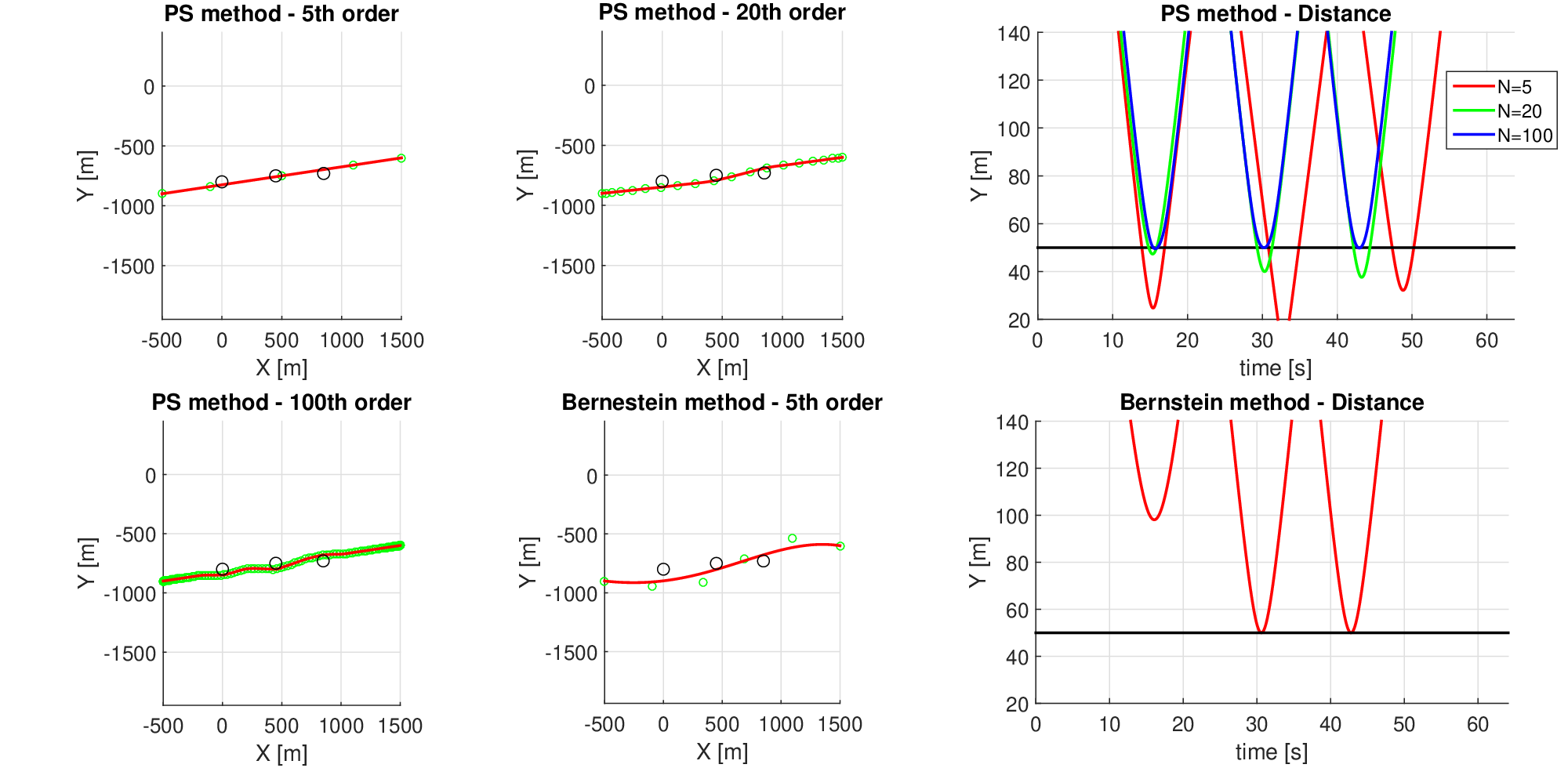
The discretization method proposed in this paper is compared to the Legendre pseudospectral method [42]. The results are enclosed in Figure 6. The top-left, top-center and bottom-left figures show the trajectories, obtained using the pseudospectral method with orders of approximation 5, 20 and 100, respectively. As discussed in the introduction, the pseudospectral method enforces the constraints only at the discretization nodes and not in between them. By increasing the number of nodes, the distance between the entire trajectory and the obstacles increases towards the desired value . However, as demonstrated by the top-right figure, which depicts the distance between the trajectories and the obstacles for the three order of approximations indicated above, the minimum separation constraint is never satisfied. On the other hand, the bottom-center figure shows that with the proposed method, even by choosing a small number of nodes (N=5 in this example), the collision avoidance constraint can be computed for the entire curve using, for example, the minimum distance algorithm introduced in Section 2, Property 4. Thus, collision avoidance is satisfied for the entire trajectory. The bottom-right figure supports this claim by showing that the distance between the trajectory and the obstacles is always greater than the required value.
8.4 Example 4 - Trajectory generation for multi-vehicle missions
As evidenced by the previous example, the possibility of choosing low order of approximations while guaranteeing constraint satisfaction is the strength of the proposed approach, which prioritizes safety and feasibility of the trajectories over optimality. The advantage of the method becomes more evident in multi-vehicle missions, where the trajectories assigned to the vehicles must be (spatially or temporally)11 1 Spatial separation is guaranteed if the minimum distance between any two points on two paths is greater than or equal to a minimum spatial clearance (the paths never intersect); temporal separation is achieved if for any time the minimum distance between two vehicles is greater than or equal to the minimum spatial clearance. separated. Consider for example a mission scenario in which vehicles, starting from their initial positions, have to follow spatially separated trajectories to reach predefined final destinations. By adopting the pseudospectral method described above, spatial separation would have to be enforced by imposing separation constraints between every node of every trajectory. Thus, the problem would have separation constraints, where is the number of nodes, and is the binomial coefficient. An increased number of nodes (dictated, perhaps, by reasons similar to the ones discussed in the previous example) would increase the complexity in the search for the optimal solution, making the pseudospectral approach practically infeasible for these types of applications. On the other hand, with the approach of this paper the constraint satisfaction is achieved independently of the number of nodes. This is discussed in the next simulation scenario.
Figure 7 illustrates the results of a multi-vehicle mission in which vehicles, starting from their initial positions, have to reach a ‘’ shaped formation while minimizing the time of arrival. The Bernstein approximation method is employed with the order of approximation . The dynamics of the th vehicle are governed by the following differential equations
| (54) |
with input and state . The input constraints are:
| (55) |
| (56) |
with , and . Finally, temporal separation constraints are imposed between each pair of trajectories, i.e.
| (57) |
, where and .
The constraints in Equations (55), (56) and (57) are computed by exploiting the properties of Bernstein polynomials. In particular, we used the minimum distance and the computation of extrema algorithms from [26, 16]. Figures 8 and 9 show the time history of the speeds and angular rates, respectively, demonstrating that the input saturation constraints are satisfied for all times.
At last, the same simulation is repeated, but the temporal separation constraint given by Equation (57) is replaced by the (more stringent) spatial separation requirement
| (58) |
. Figure 10 depicts the 2D trajectories. Figures 11 and 12 illustrate the speed and angular rate commands, respectively.


9 Conclusions
This paper proposed a numerical method to approximate nonlinear constrained optimal control problems by nonlinear programming (NLPs) using Bernstein polynomial approximation. A rigorous analysis is provided that shows convergence of the solution of the NLP to the solution of the continuous-time problem. A set of conditions are derived under which the Karush-Kuhn-Tucker multipliers of the NLP converge to the costates of the optimal control problem. This led to the formulation of the Covector Mapping Theorem for Bernstein approximation, which enables numerical computation of the costates. The theoretical findings are validated through several numerical examples, and the advantages and disadvantages of the proposed method are discussed.
Appendix
Appendix A Proof of Equation (45)
Let us focus on Equation (45a). Adding and subtracting , we have
| (59) |
Using Lemma 3 and continuity of and , the first term on the right hand side of the inequality above satisfies
where is used to denote the modulus of continuity of the product , with being a bounded function due to its continuity over a bounded domain. Denote its bound as . Notice that also is bounded, as . Then using the properties of the modulus of continuity, we get
| (60) |
where is the modulus of continuity of , and is a positive constant independent of . Furthermore, we have
| (61) |
where is the Lipschitz constant of , , , and and are the moduli of continuity of and , respectively. Combining Equations (60) and (61) with Equation (59), yields
| (62) |
which proves the bound in Equation (45a). The bounds in Equations (45b)-(45d) follow easily using an identical argument.
References
- [1] A. V. Rao, “A survey of numerical methods for optimal control,” Advances in the Astronautical Sciences, vol. 135, no. 1, pp. 497–528, 2009.
- [2] J. T. Betts, Practical methods for optimal control and estimation using nonlinear programming. SIAM, 2010.
- [3] ——, “Survey of numerical methods for trajectory optimization,” Journal of guidance, control, and dynamics, vol. 21, no. 2, pp. 193–207, 1998.
- [4] B. A. Conway, “A survey of methods available for the numerical optimization of continuous dynamic systems,” Journal of Optimization Theory and Applications, vol. 152, no. 2, pp. 271–306, 2012.
- [5] E. Polak, “Optimization: Algorithms and consistent approximations,” 1997.
- [6] A. Schwartz and E. Polak, “Consistent approximations for optimal control problems based on runge–kutta integration,” SIAM Journal on Control and Optimization, vol. 34, no. 4, pp. 1235–1269, 1996.
- [7] I. M. Ross and M. Karpenko, “A review of pseudospectral optimal control: From theory to flight,” Annual Reviews in Control, vol. 36, no. 2, pp. 182–197, 2012.
- [8] F. Fahroo and I. M. Ross, “On discrete-time optimality conditions for pseudospectral methods,” in AIAA/AAS Astrodynamics Specialist Conference and Exhibit, 2006, p. 6304.
- [9] K. Bollino, L. R. Lewis, P. Sekhavat, and I. M. Ross, “Pseudospectral optimal control: a clear road for autonomous intelligent path planning,” in AIAA Infotech@ Aerospace 2007 Conference and Exhibit, 2007, p. 2831.
- [10] Q. Gong, R. Lewis, and M. Ross, “Pseudospectral motion planning for autonomous vehicles,” Journal of Guidance, Control, and Dynamics, vol. 32, no. 3, pp. 1039–1045, 2009.
- [11] N. S. Bedrossian, S. Bhatt, W. Kang, and I. M. Ross, “Zero-propellant maneuver guidance,” IEEE Control Systems, vol. 29, no. 5, 2009.
- [12] K. Bollino and L. R. Lewis, “Collision-free multi-uav optimal path planning and cooperative control for tactical applications,” in AIAA Guidance, Navigation and Control Conference and Exhibit, 2008, p. 7134.
- [13] N. Bedrossian, S. Bhatt, M. Lammers, L. Nguyen, and Y. Zhang, “First ever flight demonstration of zero propellant maneuver (tm) attitute control concept,” in AIAA Guidance, Navigation and Control Conference and Exhibit, 2007, p. 6734.
- [14] Y. Chen, M. Cutler, and J. P. How, “Decoupled multiagent path planning via incremental sequential convex programming,” in Robotics and Automation (ICRA), 2015 IEEE International Conference on. IEEE, 2015, pp. 5954–5961.
- [15] F. Augugliaro, A. P. Schoellig, and R. D’Andrea, “Generation of collision-free trajectories for a quadrocopter fleet: A sequential convex programming approach,” in Intelligent Robots and Systems (IROS), 2012 IEEE/RSJ International Conference on. IEEE, 2012, pp. 1917–1922.
- [16] R. Choe, “Distributed cooperative trajectory generation for multiple autonomous vehicles using Pythagorean Hodograph Bézier curves,” Ph.D. dissertation, University of Illinois at Urbana-Champaign, Urbana, IL, United States, 2017, submitted.
- [17] V. Cichella, I. Kaminer, C. Walton, and N. Hovakimyan, “Optimal motion planning for differentially flat systems using Bernstein approximation,” IEEE Control Systems Letters, vol. 2, no. 1, pp. 181–186, 2018.
- [18] E. Hewitt and R. E. Hewitt, “The Gibbs-Wilbraham phenomenon: an episode in fourier analysis,” Archive for history of Exact Sciences, vol. 21, no. 2, pp. 129–160, 1979.
- [19] A. Gelb and J. Tanner, “Robust reprojection methods for the resolution of the gibbs phenomenon,” Applied and Computational Harmonic Analysis, vol. 20, no. 1, pp. 3–25, 2006.
- [20] E. Tohidi, A. Pasban, A. Kilicman, and S. L. Noghabi, “An efficient pseudospectral method for solving a class of nonlinear optimal control problems,” in Abstract and Applied Analysis, vol. 2013. Hindawi, 2013.
- [21] I. M. Ross and F. Fahroo, “Pseudospectral knotting methods for solving nonsmooth optimal control problems,” Journal of Guidance, Control, and Dynamics, vol. 27, no. 3, pp. 397–405, 2004.
- [22] C. L. Darby, W. W. Hager, and A. V. Rao, “An hp-adaptive pseudospectral method for solving optimal control problems,” Optimal Control Applications and Methods, vol. 32, no. 4, pp. 476–502, 2011.
- [23] R. T. Farouki, “The Bernstein polynomial basis: a centennial retrospective,” Computer Aided Geometric Design, vol. 29, no. 6, pp. 379–419, 2012.
- [24] H. Gzyl and J. L. Palacios, “On the approximation properties of Bernstein polynomials via probabilistic tools,” Boletın de la Asociación Matemática Venezolana, vol. 10, no. 1, pp. 5–13, 2003.
- [25] L. A. Ricciardi and M. Vasile, “Direct transcription of optimal control problems with finite elements on Bernstein basis,” Journal of Guidance, Control and Dynamics, 2018.
- [26] J.-W. Chang, Y.-K. Choi, M.-S. Kim, and W. Wang, “Computation of the minimum distance between two Bézier curves/surfaces,” Computers & Graphics, vol. 35, no. 3, pp. 677–684, 2011.
- [27] P. J. Davis, “Interpolation and approximation,” Blaisdell Pub, Co., New York, vol. 1, 1963.
- [28] S. N. Bernstein, “Démonstration du théorème de Weierstrass fondée sur le calcul des probabilités (demonstration of a theorem of Weierstrass based on the calculus of probabilities),” Communications de la Société Mathématique de Kharkov, vol. 13, no. 1, pp. 1–2, 1912.
- [29] R. Bojanic and F. Cheng, “Rate of convergence of Bernstein polynomials for functions with derivatives of bounded variation,” Journal of Mathematical Analysis and Applications, vol. 141, no. 1, pp. 136–151, 1989.
- [30] T. Popoviciu, “Sur l’approximation des fonctions convexes d’ordre supérieur,” Mathematica (Cluj), vol. 10, pp. 49–54, 1935.
- [31] P. Sikkema, “Der wert einiger konstanten in der theorie der approximation mit bernstein-polynomen,” Numerische Mathematik, vol. 3, no. 1, pp. 107–116, 1961.
- [32] M. J. D. Powell, Approximation theory and methods. Cambridge university press, 1981.
- [33] M. S. Floater, “On the convergence of derivatives of Bernstein approximation,” Journal of Approximation Theory, vol. 134, no. 1, pp. 130–135, 2005.
- [34] E. G. Gilbert, D. W. Johnson, and S. S. Keerthi, “A fast procedure for computing the distance between complex objects in three-dimensional space,” IEEE Journal on Robotics and Automation, vol. 4, no. 2, pp. 193–203, 1988.
- [35] R. Choe, “Distributed cooperative trajectory generation for multiple autonomous vehicles using pythagorean hodograph Bézier curves,” Ph.D. dissertation, University of Illinois at Urbana-Champaign, 2017.
- [36] R. F. Hartl, S. P. Sethi, and R. G. Vickson, “A survey of the maximum principles for optimal control problems with state constraints,” SIAM review, vol. 37, no. 2, pp. 181–218, 1995.
- [37] D. Garg, M. A. Patterson, C. Francolin, C. L. Darby, G. T. Huntington, W. W. Hager, and A. V. Rao, “Direct trajectory optimization and costate estimation of finite-horizon and infinite-horizon optimal control problems using a radau pseudospectral method,” Computational Optimization and Applications, vol. 49, no. 2, pp. 335–358, 2011.
- [38] Q. Gong, I. M. Ross, W. Kang, and F. Fahroo, “Connections between the covector mapping theorem and convergence of pseudospectral methods for optimal control,” Computational Optimization and Applications, vol. 41, no. 3, pp. 307–335, 2008.
- [39] B. Singh, R. Bhattacharya, and S. R. Vadali, “Verification of optimality and costate estimation using hilbert space projection,” Journal of guidance, control, and dynamics, vol. 32, no. 4, pp. 1345–1355, 2009.
- [40] E. Tohidi, O. R. N. Samadi, and M. H. Farahi, “Legendre approximation for solving a class of nonlinear optimal control problems,” Journal of Mathematical Finance, vol. 1, no. 01, p. 8, 2011.
- [41] W. Kang, Q. Gong, and I. M. Ross, “Convergence of Pseudospectral Methods for a Class of Discontinuous Optimal Control,” in 2005 IEEE 44th Conference on Decision and Control (CDC), Seville, Spain, 2005, pp. 2799–2804.
- [42] Q. Gong, W. Kang, N. S. Bedrossian, F. Fahroo, P. Sekhavat, and K. Bollino, “Pseudospectral optimal control for military and industrial applications,” in Decision and Control, 2007 46th IEEE Conference on. IEEE, 2007, pp. 4128–4142.