Quantum thermometry in a squeezed thermal bath
Abstract
We address the dephasing dynamics of the quantum Fisher information (QFI) for the process of quantum thermometry with probes coupled to squeezed thermal baths via the nondemolition interaction. We also calculate the upper bound for the parameter estimation and investigate how the optimal estimation is affected by the initial conditions and decoherence, particularly the squeezing parameters. Moreover, the feasibility of the optimal measurement of the temperature is discussed in detail. Then, the results are generalized for entangled probes and the multi-qubit scenarios for probing the temperature are analysed. Our results show that the squeezing can decrease the number of channel uses for optimal thermometry. Comparing different schemes for multi-qubit estimation, we find that an increase in the number of the qubits, interacting with the channel, does not necessarily vary the precision of estimating the temperature. Besides, we discuss the enhancement of the quantum thermometry using the parallel strategy and starting from the W state.
keywords
Entangled probes; quantum metrology; dephasing model; squeezed thermal bath.1 Introduction
Acquiring information about the world is realized by observation and measurement, and the results of which are subject to error [1]. The classical approach to decrease the statistical error is increase in the the resources for the measurement according to the central limit theorem; but this method is not always desirable or efficient [2]. Quantum parameter estimation theory describes strategies allowing the estimation precision to surpass the limit of classical approaches [3, 4, 5, 6, 7, 8, 9, 10, 11, 12]. When the quantum system is sampled N times, different strategies [13] allowing one to achieve the Heisenberg limit, can be designed such that the variance of the estimated parameter scales as . Initially entangled probes, however, may in principle offer a significant enhancement in precision of parameter estimation [13, 14, 15, 16, 17, 18]. Those strategies have been realized experimentally in atomic spectroscopy [19, 20] in which the spin-squeezed states have been employed for improving frequency calibration precision [21, 22]. Besides, the same quantum enhancement principle can be utilized in optical interferometry [23, 24] with exciting applications in the process of seeking the first direct detection of gravitational waves [25].
On the other hand, it has been also proven the entanglement is not always useful for parameter estimation [26] and there are highly entangled pure states that are not useful in the process of quantum estimation. Moreover, it has been discussed [3] while entanglement at the initial stage can be useful to enhance the precision of the estimation, entangled measurements are never necessary. Besides, there are some cases in which if the probes are initially prepared in an unentangled state, a better performance for the parameter estimation is attainable [27]. Specifically, in Ref. [13] it has been illustrated that in the presence of Pauli x-y, depolarizing, and amplitude damping noise, unentangled probes perform better in the high-noise regime. Particularly, the view that entanglement is necessary for quantum-enhanced metrology has been challenged in Refs. [28, 29] by demonstrating that the enhancement, obtained via entanglement, may be contingent on the final measurement and the way in which the unknown parameter is encoded into the probe quantum state. In addition, it has been illustrated that under certain conditions the entanglement may even lead to deleterious effects in quantum metrology [30]. According to the above discussion, presenting a universal prescription, applicable for all quantum systems, about the relation between the QFI and entanglement, is not possible. These reasons motivate us to investigate more the role of the entanglement in different quantum scenarios for quantum metrology.
Recently, the quantum parameter estimation theory have attracted increasing attention in the field of quantum thermodynamics in which accurate estimation and control of the temperature are very significant [31, 32, 33, 34]. In addition to the emergence of primary and secondary thermometers based on precisely machined microwave resonators [35, 36], recent studies have been focused on measuring temperature at even more smaller scales in which nanosize thermal baths are extremely sensitive to disturbances induced by the probes [37, 38, 39, 40, 41]. Some interesting paradigms of nanoscale thermometry are quantum harmonic oscillators [42] nanomechanical resonators [43], and atomic condensates [44, 45]. On the other hand, temperature plays an important role in realizing phase-matching condition in non-linear optical materials. Besides, thermal processes may result in large nonlinear optical effects originated from temperature dependence of the material refractive index [46]. Accordingly, precise determination of the temperature is of great importance in all branches of modern science and technology [47, 48, 49]. A scheme for enhancing the sensitivity of quantum thermometry is proposed in [50] where the sensing quantum system used to estimate the temperature of an external bath is dynamically coupled with an external ancilla (a meter) via a Hamiltonian term. Moreover, the dephasing dynamics of a single-qubit as an effective process in order to estimate the temperature of its environment is addressed in [51]. Here, we generalize the results by using the entangled probes in the presence of squeezed noises [52] which are of great importance for the thermometry of the thermal bath. In particular, investigating the quantum metrology in the presence of these quantum noises completes other studies focusing on exploring the characterization of complex environments described classically [53, 54, 55, 56, 57].
One of the main design considerations in digital electronics is energy dissipation. According to Landauer’s principle [58], the erasure (or reset) of one bit of classical information is necessarily associated with an energy input of at least and an entropy increase of at least . On the other hand, it is predicted that the Landauer limit will be achieved within the next few decades [59]. Therefore, improving our understanding of energy dissipation in information processing devices are of both theoretical and technological interest. Because of the advancing miniaturization, nonequilibrium and quantum effects must be also taken into account [60, 61]. Moreover, it has been demonstrated [62] that memory devices embedded in a squeezed thermal reservoirs [63] are unbounded by the Landauer limit. In such environments, thermal fluctuations exhibit fast periodic amplitude modulations, which can be used to decrease the minimum energy costs for an erasure operation below the standard Landauer limit. This setup can naturally arise in digital electronic circuits operating in a pulse-driven fashion and, in the future, might be exploited to build more energy-efficient electronic devices. Besides, in the context of heat engines, it has been suggested that [64] squeezed thermal states may be exploited as an additional resource to overcome the standard Carnot limit [65] bounding the efficiency of heat engines; particularly, in Ref. [52] a nanobeam heat engine coupled to squeezed thermal noise has been realized, whose efficiency is not bounded by the standard Carnot limit.
According to above discussion, appearance of squeezed noise in future advanced devices is unavoidable, leading to destroy the equilibrium nature of the thermal state because of fast periodic modulations of the temperature. Thus, estimating the initial temperature of the thermal bath driven by the squeezed noise is of great practical importance.
In this work, we propose a thermometer, consisting N qubits for probing the initial temperature of a thermal bath disturbed by the squeezed noise and calculate the bounds on the quantum thermometry in the presence of squeezing. It is supposed that qubits are directly coupled to the thermal bath of interest and qubits are not directly coupled to the bath but instead serve as an information storage which may be read out at the final time . Our scheme relies on the possibility of performing joint measurements on all of qubits. The model is well adopted to describe physical systems such as the molecular oscillation, exciton-phonon interaction, and photosynthesis process [66, 67, 68]. Analytically, we investigate the effects of the initial state or squeezing and other environmental parameters on the estimation of the temperature. Besides, we extend our study to multiqubit estimation realized by initially entangled probes and address the role of entanglement in the process of thermometry on the squeezed thermal bath.
This paper is organized as follows: In Secion 2, we present a brief review of the QFI and obtain the upper bound for the quantum parameter estimation. The model is introduced in Section 3. Different scenarios for quantum thermometry are discussed completely in Section 4. Finally in Section 5, the main results are summarized.
2 The Preliminaries
2.1 (Quantum) Fisher information
The classical Fisher information is an important method of measuring the amount of information which an observable random variable carries about unknown parameter . Supposing that denotes the probability distribution with measurement outcomes , the classical Fisher information is defined as [69]:
| (1) |
characterizing the inverse variance of the asymptotic normality of a maximum-likelihood estimator. If observable is continuous, the summation should be replaced by an integral.
The quantum analog of the Fisher information can be formally generalized from Eq. (1) such that it is defined as [70]:
| (2) |
in which the symmetric logarithmic derivative (SLD) operator represents a Hermitian operator determined by
| (3) |
where denotes the anti-commutator. Considering the density matrix spectral decomposition as , associated with as well as , and focusing on the following formula for the QFI:
| (4) |
we can rewrite the QFI as [71]
| (5) |
where in the first and second summations we should exclude sums over all and , respectively.
According to quantum Cramér-Rao (QCR) theorem, a significant property of the QFI is that we can obtain the achievable lower bound of the mean-square error of the unbiased estimator for parameter T, i.e.,
| (6) |
in which denotes the unbiased estimator, and represents the number of repeated experiments.
2.2 Upper bound for parameter estimation
Given an initial pure state , we know that it evolves according to the expression , where ’s represent -dependent Kraus operators [72]. It has been derived that the upper bound to the QFI is given by [73]:
| (7) |
where
| (8) |
| (9) |
and .
3 The Model
At first, we introduce the dephasing model [74], composed of a two level system interacting with a boson bath . The interaction of system-bath (S-B) can be described by Hamiltonian , where and are the ground and excited states, respectively. Because ; the energy of the system is conserved, and hence the population of energy levels do not change with time.
Starting from , we focus on the case in which the initial state of the boson bath is a squeezed thermal state [75]
| (10) |
in which T represents the temperature of the thermal bath prepared in the state , denotes the normalization constant, and represents the squeezing operator for the boson bath, where denotes the squeezing operator corresponding to mode [63]:
| (11) |
where and represent the squeezing strength and phase parameters, respectively.
In the interaction picture, the evolved reduced density matrix can be obtained as
| (12) |
where is the population of excited level and denotes the decay factor. We focus on the Ohmic environment where its coupling spectral density , whose summation should be written as an integral for continuous bath modes, is given by in which denotes the cutoff frequency and is a unitless number representing the coupling strength.
Defining where and assuming that and , we can find that the decay factor is given by [76]
| (13) |
where, as described before, represents the squeezing strength, characterizes the S-B coupling strength, and denotes the phase difference between the squeezing phase relative to the phase of the coupling strength. Moreover, the time-dependent coefficients are of the form
| (14) |
where
and where
| (15) |
| (16) |
in which and .
4 Scenarios for quantum thermometry



4.1 Single-qubit scenario
Our model describes a dephasing channel such that the system can be used for probing temperature of the thermal bath. In the first scenario in which the single-qubit is used for thermometry, the corresponding QFI is obtained as follows:
| (17) |
where the partial derivative is given by
| (18) |
in which
| (19) |
where .
Preparing the qubit probe in a pure state , the QFI reduces to the following expression:
| (20) |
saturating the upper bound obtained from Eq. (7) for . Throughout this paper, we set and normalize the QFI for clearer illustration.
Although our approach for computing the analytical results is completely general, we limit our study of the QFI behaviour to the high-T Ohmic reservoir. Therefore, all QFI figures are plotted and interpreted in this regime. In the high-temperature limit that and , it is found that
| (21) |
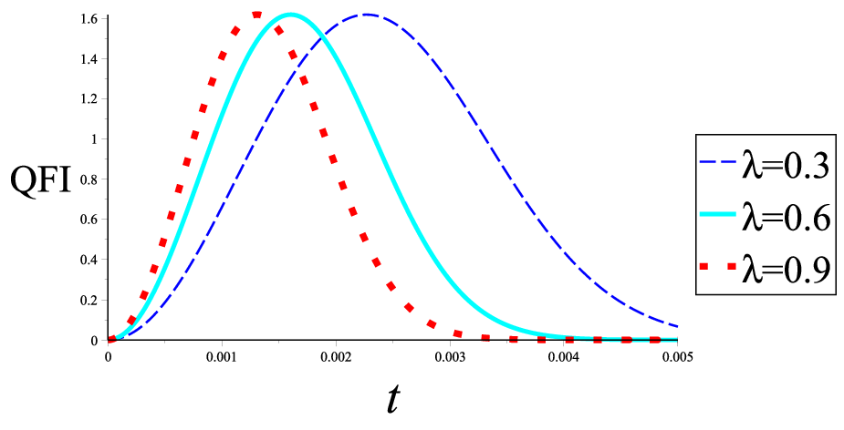
Investigating the QFI as a function of time, we find that at first it increases, reaching a maximum (see Figs. 1-3). According to theory of quantum metrology, an increase in QFI means that the precision of quantum estimation is improved. This originates from the fact that interaction of the qubit with the bath encodes the information about the temperature into the quantum state of the probe, hence the QFI increases. However, because of the decoherence effects, the encoded information flows from the system to the environment, and hence its destructive influence appears and the QFI falls, thus, the quantum thermometry becomes more inaccurate.
We first investigate the behaviour of the QFI dynamics with respect to cutoff frequency and S-B coupling strength . As shown in Figs. 1 and 1, the variation of theses parameters can not change the maximum value of the QFI. Therefore, the optimum precision obtained in the process of thermometry does not vary. However, the figure shows when the cutoff frequency or the coupling increases, the maximum point of the QFI is shifted to the left, and hence the QFI reaches its maximum value sooner. Although increase of the coupling between the probe and the bath or increasing the cutoff frequency decreases the interaction time for obtaining the optimal estimation precision, the QFI decreases more quickly, and hence the time period that we can extract the information about the temperature is shortened.
Squeezing effects of increasing squeezing strength are shown in Fig. 2. We can achieve sooner the optimal precision of thermometry probing more squeezed fields such that the optimal value of the QFI also remains invariant. Interestingly, Fig. 2 illustrates that in more squeezed fields the optimal estimation is attainable with more weak coupling between the probe and the bath. This may leads to important results in improving the control of decoherence in the process of quantum communication.
Now we investigate how may affect the dynamics of the QFI. As shown in Fig. 3, when the relative phase varies from to rad, the interaction time between the probe and the bath can be reduced and hence the optimal value of estimation, not affected by variation of the relative phase, is obtained sooner. However, varying the relative phase from to , we see that the maximum point, at which the QFI is maximized, can be shifted to the right. Therefore, the QFI reaches its maximum value at a later time-point. Nevertheless, Fig. 3 exhibits a positive and interesting consequence of increasing the relative phase from to . We see that larger relative phases lead to retardation of the QFI loss during the time evolution and therefore enhance the estimation of the parameter at a later time.
4.1.1 Feasible measurement for optimal estimation
Another important question is how we can practically design the optimal estimation, i.e., a practically feasible measurement whose Fisher information is equal to the QFI. For answering this question, we should compute the SLD, since the optimal POVM can be constructed by the eigenvectors of the SLD [6, 10]. Using Eq. (12) and following the approach introduced in [77] for computing the SLD of one-qubit systems, we find that the SLD associated with the thermometry is given by
| (22) |
When the qubit probe is prepared initially in a pure state , some interesting results may be extracted. In particular, for , the SLD reduces to the following compact form:
| (23) |
For ( ), the above SLD commutes with and they have common eigenvectors, i.e., measurement of leads to the optimal estimation of the temperature, because an optimal measurement can be performed if we measure in the eigenbasis of the SLD [78].
4.2 Multi-qubit scenario
For our dephasing model, it is simple to obtain the operator-sum representation where the time-dependent Kraus operators are given by
| (24) |
Two usual scenarios in which probes are submitted to independent processes are shown in Fig. 4 for estimating the temperature. In both parallel and ancilla-assisted strategies shown in Figs. 4 and 4, using the above Kraus operators, we find that and introduced, respectively, in Eqs. (8) and (9) are given by:
| (25) |
where denotes identity operator acting on -dimensional Hilbert space. Inserting these equations into (7), one obtains the upper bound for the QFI associated with the temperature as follows:
| (26) |
where in the parallel strategy, we put . Although the use of the noiseless ancillas does not improve the upper bound for the QFI, we cannot necessarily conclude that the parallel strategy leads to more accurate estimation than the ancilla-assisted one. We will come back to discuss this problem, after obtaining the exact expressions for the QFIs.
In the first scenario, we adopt the ancilla-assisted strategy in the sense that the probes are realized with two qubits such that one of which is noiseless ( see Fig. 4 with , and ). Because this is the model for two independent environments, the Kraus operators are just tensor products of Kraus operators of each of the qubits, . Preparing initially the qubits in the Bell state , we find that the output state of the channel, measured for estimating the temperature, is given by
| (27) |
Therefore, the corresponding QFI denoted by , is obtained as
| (28) |
saturating the upper bound. In the parallel scenario in which both qubits are affected by the noise, the QFI is given by:
| (29) |
The saturation of the upper bound in the ancilla-assisted strategy indicates that this scenario may sometimes lead to more accurate estimation than the parallel one.
An important difference between bipartite entanglement and multipartite one is how they are classified. Greenberger-Horne-Zeilinger (GHZ) state [79], W state [80] are two typical classes of multipartite entangled states needed for different quantum information processing tasks. For instance, GHZ states are the best quantum channels for teleportation [81] or quantum key distribution [82], and W states are required for secure quantum communication [83, 84]. Moreover, the entanglement of W state is robust against disposal of particles [80]. Besides, the W state plays an important role in the leader election problem in anonymous quantum networks [85]. It has been also shown that the quantum coherence of W states leads to high efficiency in quantum thermalization of a single mode cavity [86].
Using a three-qubit probe () with , and , initially prepared in the GHZ state , we again the same result for , i.e.,
| (30) |
On the other hand, if the probes are initially in the W state the QFI is given by
| (31) |
Therefore, and it cannot saturate the upper bound.


Natural generalizations of the GHZ and W states to N-qubit systems are
| (32) |
| (33) |
Starting from initial state such that qubits are affected by the channel and using Eq. (5) for computing the QFI corresponding to the temperature estimation, we find that the second term in right hand side of (5) is always zero because the eigenvectors of the evolved density matrix are -independent. Moreover, all the eigenvalues except two vanish, simplifying the computation of the QFI. Hence, simultaneously using Mathematica and QUBIT4MATLAB V5.6 [87] to work with the high-dimensional density matrices, we find that the corresponding QFI for any choice of is obtained as follows:
| (34) |
Clearly, an increase in the number of the noiseless qubits does not affect the accuracy of the estimation. The above formula can be generalized to parallel strategy as follows:
| (35) |


As seen in Fig. 5, we find that in the parallel strategy with initial GHZ state, an increase in , the number of uses of the channel, does not necessarily enhance the QFI and it may even lead to decrease of the precision of the temperature estimation. We address how the optimal number of interacting qubits with which the QFI is maximized, is affected by other parameters. Our computation shows that the optimal value of , is given by
| (36) |
where denotes the principal solution for in and R(x) rounds to the nearest integer. If the above formula leads to value smaller than 3, we conclude that the best estimation occurs for N=3.
For initial GHZ state, we find that very squeezed fields needs less qubits for achieving optimal estimation of the temperature (see Fig. 5). Nevertheless, it should be noted that the squeezing first leads to increase in the number of channel uses for achieving the optimal thermometry. However, more squeezing, corresponding to values of larger than some critical value , reverses the process, and consequently it decreases the number of uses of the channel. Moreover, as shown in Fig. 5, when the relative phase increases from to rad, the number of uses of the channel can be reduced and the optimal value of estimation, not affected by variation of the relative phase, is obtained with less qubits interacting with the bath. Similarly, it is found that when the S-B coupling is strengthened, the optimal for which the QFI is maximized decreases. Therefore, if the interacting qubits are weakly coupled to the bath the cost of quantum thermometry may increase.
On the other hand, starting from state such that one of the qubits is affected by the channel (n=1) and computing the spectral decomposition of the evolved density matrix, one finds that all the eigenvalues (eigenvectors) except two vanish (are -independent), resulting in the following simple expression of the QFI for any choice of :
| (37) |
It is obvious that the upper bound can never be saturated in this situation. Hence, when one of the qubits is affected by the channel, the single-probe strategy leads to more precise estimation than the ancilla-assisted one started from the W state:
| (38) |
Therefore, the entangled strategy is not always more efficient than the single-qubit one for quantum thermometry.
In the parallel strategy, starting from and diagonalizing the evolved density matrix, again we see that all the eigenvectors are -independent and all the eigenvalues except vanish. Hence, one can find that the QFIs corresponding to different parallel strategies satisfy
| (39) |

Plotting as a function of illustrates that the QFI is enhanced when the number of the channel uses increases. Increasing can also raise the efficiency of the parallel strategy with initial W state with respect to the single-qubit strategy for quantum thermometry (see Fig. 6).
For , a compact expression for is not generally accessible except for some special cases presented here briefly:
| (40) |
| (41) |
| (42) |
| (43) |
| (44) |


According to Eq. (38), it is concluded that for , starting from the GHZ state or adopting the single-qubit strategy, we achieve more accurate estimation than starting from W state. However, for , initial preparation of the probes in W state leads to more efficient thermometry than starting with GHZ state (see Fig. 7).
Now an important question arises: are the GHZ and W states the optimal one? Are there (entangled) states which lead to more accurate estimation? The answer to this question cannot be analytic, since the analytical diagonalization of a multi-qubit density matrix is not generally possible. In order to solve this problem, we should attack it numerically and first notice that the QFI is maximized for an initial pure state [88]. After generating a large number of random initial pure states by QUBIT4MATLAB V5.6 [87], we find that the QFI, evaluated numerically using expression (4), is maximized for either GHZ or W states for N = 2,3,4,5,6. Nevertheless, our limited observations should not be understood as a certain result, because the general answer can be presented only when we can check all the initial states while solving the eigenvalue problem for high-dimensional density matrices leads to some complexity in the process of computing the QFI. Moreover, the iterative method discussed in Ref. [89] also bypasses the direct maximization of the QFI, however, that method is only designed for those quantum channels that can be represented as (in which denotes a noisy channel) under certain assumptions and for estimating .
5 Summary and conclusions
To summarize, we discussed in detail the quantum thermometry by using a qubit subjected to the dephasing dynamics via interacting with a squeezed thermal bath. In particular, it was investigated how we can practically design the optimal estimation for one-qubit probe. Moreover, we illustrated that the optimum precision obtained in the process of thermometry is robust against squeezing. In addition, it was shown that squeezing parameters lead to interesting and non-trivial effects on the quantum thermometry. Generalizing the results for entangled probes and analysing the multi-qubit strategies for estimating the temperature, we found that that in the entangled strategy with initial GHZ state, an increase in the number of uses of the channel, does not necessarily enhance the QFI and it may even lead to decrease of the precision of the temperature estimation. Moreover, the squeezing may decrease the thermometry costs. We also addressed how the parallel strategy starting from the W state becomes more efficient than the single-qubit strategy for quantum thermometry.
6 Acknowledgements
I wish to acknowledge the financial support of the MSRT of Iran and Jahrom University.
References
- [1] C. W. Helstron, Quantum detection and estimation theory (Academic Press, 1976).
- [2] Y. Israel, S. Rosen, and Y. Silberberg, Phys. Rev. Lett. 112, 103604 (2014).
- [3] V. Giovannetti, S. Lloyd, and L. Maccone, Phys. Rev. Lett. 96, 010401 (2006).
- [4] V. Giovannetti, S. Lloyd, and L. Maccone, Science 306, 1330 (2004).
- [5] W. van Dam, G. M. D’Ariano, A. Ekert, C. Macchiavello, and M. Mosca, Phys. Rev. Lett. 98, 090501 (2007).
- [6] M.G.A. Paris, Int. J. Quant. Inf. 7, 125 (2009).
- [7] H. Rangani Jahromi, M. Amniat-Talab, Ann. Phys. 355, 299 (2015).
- [8] H. Rangani Jahromi and M. Amniat-Talab, Ann. Phys. 360, 446461 (2015).
- [9] H. Rangani Jahromi, J. Mod. Opt. 64, 1377 (2017).
- [10] H. Rangani Jahromi, Opt. Commun. 411, 119 (2018).
- [11] M. Jafarzadeh, H. Rangani Jahromi, and M. Amniat-Talab, Quantum Inf. Process 17, 165 (2018).
- [12] H. Rangani Jahromi, arXiv:1807.09362.
- [13] Z. Huang, C. Macchiavello, and L. Maccone, Phys. Rev. A 97, 032333 (2018).
- [14] R. Demkowicz-Dobrzański, J. Kolodyński, and M. Guta, Nature Comm. 3, 1063 (2012).
- [15] D. W. Berry, and H. M. Wiseman, Phys. Rev. Lett. 85, 5098–5101 (2000).
- [16] M.Zwierz, C. A.Prez-Delgado and P. Kok, Phys. Rev. Lett. 105, 180402 (2010).
- [17] R. Demkowicz-Dobrzański, and L. Maccone, Phys. Rev. Lett. 113, 250801 (2014).
- [18] G.-Q. Liu, Y.-R. Zhang, Y.-C. Chang, J.-D. Yue1, H. Fan, and X.-Y. Pan, Nature Comm. 6, 6726 (2015).
- [19] D. J. Wineland, W. M. Itano, J. J. Bollinger, and F. L. Moore, Phys. Rev. A 46, R6797 (1992).
- [20] S. F. Huelga, C. Macchiavello, T. Pellizzari, and A. K. Ekert, Phys. Rev. Lett. 79, 3865 (1997).
- [21] W. Wasilewski, K. Jensen, H. Krauter, J. J. Renema, M. V. Balabas, and E. S. Polzik, Phys. Rev. Lett. 104, 133601 (2010).
- [22] M.Koschorreck, M. Napolitano, B.Dubost, and M. W.Mitchell, Phys. Rev. Lett. 104, 093602 (2010).
- [23] M. W. Mitchell, J. S. Lundeen, and A. M.Steinberg, Nature 429, 161 (2004).
- [24] T. Nagata, R.Okamoto, J. L. O’Brien, K. Sasaki, and S. Takeuchi, Science 316, 726 (2007).
- [25] LIGO Collaboration, Nat. Phys. 7, 962 (2011).
- [26] P. Hyllus, O. Gühne and A. Smerzi, Phys. Rev. A 82 012337 (2010).
- [27] S. Boixo, A. Datta, M. J. Davis, S. T. Flammia, A. Shaji, and C. M. Caves, Phys. Rev. Lett. 101 040403 (2008).
- [28] T. Tilma, S. Hamaji, W. J. Munro, and K. Nemoto, Phys. Rev. A 81, 022108 (2010).
- [29] A. Datta and A. Shaji, Mod. Phys. Lett. B 26, 1230010 (2012).
- [30] J. Sahota and N. Quesada, Phys. Rev. A 91, 013808 (2015).
- [31] N. S. Williams, K. Le Hur, and A. N. Jordan, J. Phys. A: Math. Theor. 44, 385003 (2011).
- [32] M. Kliesch, C. Gogolin, M. J. Kastoryano, A. Riera, and J. Eisert, Phys. Rev. X 4, 031019 (2014).
- [33] J. Millen and A. Xuereb, New J. Phys. 18, 011002 (2016).
- [34] S. Vinjanampathy and J. Anders, Contemp. Phys. 57, 545 (2016).
- [35] P. J. Mohr and B. N. Taylor, Rev. Mod. Phys. 77, 1 (2005).
- [36] W. Weng, J. D. Anstie, T. M. Stace, G. Campbell, F. N. Baynes, and A. N. Luiten, Phys. Rev. Lett. 112, 160801 (2014).
- [37] A. De Pasquale, D. Rossini, R. Fazio, and V. Giovannetti, Nat. Commun. 7, 12782 (2016).
- [38] A. De Pasquale, K. Yuasa, and V. Giovannetti, Phys. Rev. A 96, 012316 (2017).
- [39] B. Farajollahi, M. Jafarzadeh, H. Rangani Jahromi, and M. Amniat-Talab, Quant. Inf. Proc. 17, 119 (2018).
- [40] S. Campbell, M. Mehboudi, G. De Chiara, and M. Paternostro, New J. Phys. 19, 103003 (2017).
- [41] G. De Palma, A. De Pasquale, and V. Giovannetti, Phys. Rev. A 95, 052115 (2017).
- [42] M. Brunelli, S. Olivares, M. Paternostro, and M. G. A. Paris, Phys. Rev. A 86, 012125 (2012).
- [43] M. Brunelli, S. Olivares, and M. G. A. Paris, Phys. Rev. A 84, 032105 (2011).
- [44] T. H. Johnson, F. Cosco, M. T. Mitchison, D. Jaksch, and S. R. Clark, Phys. Rev. A 93, 053619 (2016).
- [45] M. Hohmann, F. Kindermann, T. Lausch, D. Mayer, F. Schmidt, and A. Widera, Phys. Rev. A 93, 043607 (2016).
- [46] R. Boyd, Nonlinear Optics, (Academic Press, 2008).
- [47] P. Neumann, I. Jakobi, F. Dolde, C. Burk, R. Reuter, G. Waldherr, J. Honert, T. Wolf, A. Brunner, J. H. Shim, et al., Nano Lett. 13, 2738 (2013).
- [48] G. Kucsko, P. Maurer, N. Yao, M. Kubo, H. Noh, P. Lo, H. Park, and M. Lukin, Nature 500, 54(2013) .
- [49] D. M. Toyli, F. Charles, D. J. Christle, V. V. Dobrovitski, and D. D. Awschalom, Proc. Natl. Acad. Sci. USA 110, 8417 (2013).
- [50] A. H. Kiilerich, A. D. Pasquale, and V. Giovannetti, Phys. Rev. A 98, 042124 (2018).
- [51] S. Razavian, C. Benedetti, M. Bina, Y. Akbari-Kourbolagh, Matteo G. A. Paris, arXiv:1807.11810v1.
- [52] J. Klaers, S. Faelt, A. Imamoglu, and E. Togan, Phys. Rev. X 7, 031044 (2017).
- [53] C. Benedetti, F. Buscemi, P. Bordone, M.G.A. Paris, Phys. Rev. A 89, 032114 (2014).
- [54] C. Benedetti, M.G.A. Paris, Phys. Lett. A 378, 2495 (2014).
- [55] M.A.C. Rossi, M.G.A. Paris, Phys. Rev. A 92, 010302(R) (2015).
- [56] M. Javed, S. Khan, S.A. Ullah, Quantum Inf. Process. 17, 53 (2018)
- [57] L. T. Kenfack, M. Tchoffo,L. C. Fai, Phys. Lett. A 383, 1123 (2019).
- [58] R. Landauer, IBM J. Res. Dev. 5, 183 (1961).
- [59] E. Pop, Nano Res. 3, 147 (2010).
- [60] J. Goold, M. Paternostro, and K. Modi, Phys. Rev. Lett. 114, 060602 (2015).
- [61] G. Manzano, Eur. Phys. J. Spec. Top. 227, 285 (2018).
- [62] J. Klaers, Phys. Rev. Lett. 122, 040602 (2019).
- [63] M. O. Scully, and M. S. Zubairy, Quantum Optics (Cambridge Univ. Press, 1997)
- [64] J. Rossnagel, O. Abah, F. Schmidt-Kaler, K. Singer, and E. Lutz, Phys. Rev. Lett. 112, 030602 (2014).
- [65] S. Carnot, Réflexions sur la Puissance Motrice du feu et sur les Machines Propres a Développer Cette Puissance (Bachelier, Paris, 1824).
- [66] H. Dong, S.-W. Li, Z. Yi, G. S. Agarwal, and M. O. Scully, arXiv:1608.04364.
- [67] H. Dong, D.-W. Wang, and M. B. Kim, arXiv:1706.02636.
- [68] V. May and O. Kühn, Charge and Energy Transfer Dynamics in Molecular Systems: A Theoretical Introduction, 1st ed. (Wiley-VCH, Berlin, 2000).
- [69] C. W. Helstrom, Quantum Detection and Estimation Theory (Academic, New York, 1976).
- [70] V. Giovannetti, S. Lloyd, and L. Maccone, Phys. Rev. Lett. 96, 010401 (2006).
- [71] W. Zhong, Z. Sun, J. Ma, X. Wang, and F. Nori, Phys. Rev. A 87, 022337 (2013).
- [72] M. A. Nielsen and I. L. Chuang, Quantum Computation and Quantum Information (Cambridge University Press, Cambridge, 2000).
- [73] B. M. Escher, R. L. de Matos Filho, and L. Davidovich, Nat. Phys. 7, 406 (2011).
- [74] H. Breuer and F. Petruccione, The Theory of Open Quantum Systems (Oxford University Press, Oxford, 2002).
- [75] S. Banerjee and R. Ghosh, J. Phys. A: Math. Theor. 40, 13735 (2007).
- [76] Yi-Ning You and Sheng-Wen Li, Phys. Rev. A 97, 012114 (2018).
- [77] F. Chapeau-Blondeau, Phys. Rev. A 91, 052310 (2015).
- [78] G. Tóth and L. Apellaniz, J. Phys. A: Math. Theor. 47, 424006 (2014).
- [79] D. M. Greenberger, M. A. Horne, A. Shimony, and A. Zeilinger, Am. J. Phys. 58, 1131 (1990).
- [80] W. Dür, Phys. Rev. A 63, 020303(R) (2001).
- [81] Z. Zhao, Y.-A. Chen, A.-N. Zhang, T. Yang, H. J. Briegel, and J-W. Pan, Nature. 430, 54 (2004).
- [82] J. Kempe, Phys. Rev. A 60, 910 (1999).
- [83] J. Wang, Q. Zhang, and C.-J. Tang, Commun. Teor. Phys. 48, 637 (2007).
- [84] W. Liu, Y. B. Wang, and Z. T. Jiang, Opt. Commun. 284, 3160 (2011).
- [85] E. D’Hondt, and P. Panangaden, Quantum Inf. Comput. 6, 173 (2006).
- [86] C. B. Daǧ, W. Niedenzu, Ö. E. Müstecaplıoǧlu, and G. Kurizki, Entropy 18, 244 (2016).
- [87] G. Tóth, Comput. Phys. Commun. 179, 430 (2008).
- [88] A. Fujiwara, Phys. Rev. A 63, 042304 (2001).
- [89] K. Macieszczak, arXiv:1312.1356.