The maximal current carried by a normal/superconducting interface in the absence of magnetic field

L. K. HART Thanks: Department of Mathematics, Louisiana State University, Baton Rouge, LA 70803, USA. Y. ALMOG Thanks: Department of Mathematics, Ort-Braude College, Carmiel 21610, Israel

Abstract: Modeling a normal/superconducting interface, we consider a semi-infinite wire whose edge is adjacent to a normal magnetic metal, assuming asymptotic convergence, away from the boundary, to the purely superconducting state. We obtain that the maximal current which can be carried by the interface diminishes in the small normal conductivity limit.

1 Introduction

Consider a superconducting wire placed at a temperature lower than the critical one. It is well-known that at such temperatures the superconductor loses its electrical resistivity. This means that a current can flow through a superconducting sample and generate a vanishingly small voltage drop. If one increases the current beyond a certain critical threshold, the material will revert to the normal state, even if the temperature is kept fixed below the critical level.

In the absence of magnetic field, the critical current density, at which superconductivity is destroyed, has been obtained in the physics literature (cf. [14, 6] and also (4) below) by neglecting the effect of boundaries. Consequently, this critical current density does not depend at all on the normal conductivity of the wire, a result which appears to be counter-intuitive. It is of interest, therefore, to examine how an interface with a normal magnetic metal affects the critical current density and to estimate the potential drop over such an interface.

Consider, then, a superconductiong wire, denoted by $\Omega$ . The wire has interface $\partial\Omega_{c}$ with a magnetic metal which is at normal state. The remaining boundary $\partial\Omega_{i}$ is adjacent to an insulator. To obtain the critical current density we use the time-dependent Ginzburg-Landau model in the absence of a magnetic field, presented here in the dimensionless form [2, 8, 12] (cf. [2] for a formal justification of the model).


$\displaystyle\frac{\partial\psi}{\partial t}+i\phi\psi=$	$\displaystyle\;\Delta\psi+\psi(1-\|\psi\|^{2})$	$\displaystyle\text{in}\;\Omega\;\text{x}\;\mathbb{R}_{+}$	(1a)
$\displaystyle\sigma\Delta\phi=$	$\displaystyle\;\nabla\,\cdot[\Im(\bar{\psi}\nabla\psi)]$	$\displaystyle\text{in}\;\Omega\;\text{x}\;\mathbb{R}_{+}$	(1b)
$\displaystyle\psi=$	$\displaystyle\;0$	$\displaystyle\text{on}\;\partial\Omega_{c}\;\text{x}\;\mathbb{R}_{+}$	(1c)
$\displaystyle-\sigma\frac{\partial\phi}{\partial v}=$	$\displaystyle\;J$	$\displaystyle\text{on}\;\partial\Omega_{c}\;\text{x}\;\mathbb{R}_{+}$	(1d)
$\displaystyle\frac{\partial\psi}{\partial v}=$	$\displaystyle\;0$	$\displaystyle\text{on}\;\partial\Omega_{i}\;\text{x}\;\mathbb{R}_{+}$	(1e)
$\displaystyle\frac{\partial\phi}{\partial v}=$	$\displaystyle\;0$	$\displaystyle\text{on}\;\partial\Omega_{i}\;\text{x}\;\mathbb{R}_{+}$	(1f)
$\displaystyle\psi(x,0)=$	$\displaystyle\;\psi_{0}$	$\displaystyle\text{in}\;\Omega$	(1g)

In (1) $\psi$ denotes the superconductivity order parameter, which implies that $|\psi|^{2}$ is proportional to the number density of pairs of superconducting electrons (Cooper pairs). Superconductors with $|\psi|=1$ are called purely superconducting, whereas those for which $\psi=0$ are said to be at the normal state. The scalar electric potential is denoted by $\phi$ , while the constant $\sigma$ represents the normal conductivity of the superconducting material. In the presence of magnetic field the normal current is given by $-\sigma(\text{A}_{t}+\nabla\phi)$ , where $A$ is the magnetic vector potential, but since in our case $A=0$ the normal current is given by $-\sigma\nabla\phi$ . The function $J:\partial\Omega_{c}\to\mathbb{R}$ represents the normal current entering the sample.

The above model, with various boundary conditions, has been studied by both physicists [8, 9, 10, 5] and mathematicians [3, 13, 11, 4]. We mention in particular [2] which addresses precisely the same one-dimensional simplification we consider in the sequel.

Assuming a one-dimensional wire lying in $\mathbb{R}_{+}$ , a stationary solution of (1) must satisfy


$\displaystyle-\psi^{\prime\prime}+i\phi\psi-\psi(1-\|\psi\|^{2})=$	$\displaystyle\;0$	$\displaystyle\text{in}\;\mathbb{R}_{+}$	(2a)
$\displaystyle-\sigma\phi^{\prime\prime}+\Im[\psi^{\prime}\bar{\psi}]^{\prime}=$	$\displaystyle\;0$	$\displaystyle\text{in}\;\mathbb{R}_{+}$	(2b)
$\displaystyle\psi(0)=$	$\displaystyle\;0$	$\displaystyle-\sigma\phi^{\prime}(0)=J$	(2c)
$\displaystyle\|\psi\|\to$	$\displaystyle\rho_{\infty}$	$\displaystyle\text{as}\;x\to\infty$	(2d)
$\displaystyle\phi\to$	$\displaystyle 0$	$\displaystyle\text{as}\;x\to\infty$	(2e)

In (2), the current $J$ is constant. The boundary conditions at $x=0$ represent an interface with a magnetic metal at the normal state [14, Eq. (4.15a)]. As $x\to\infty$ the sample assumes the fully superconducting state. The latter is given, for this simple setting (cf. [2, 14]) by

\psi_{s}=\rho_{\infty}e^{i\alpha x}\hskip 14.22636pt;\hskip 14.22636pt\phi\equiv 0,

(3)

with $\alpha=[1-\rho^{2}_{\infty}]^{1/2}$ . As the superconducting current is given by $J=\Im[\psi^{\prime}_{s}\bar{\psi}_{s}]$ we must have that

J^{2}=\rho^{4}_{\infty}(1-\rho^{2}_{\infty}).

(4)

Accordingly, in (2), $J$ and $\rho_{\infty}$ must be related by (4). It can be easily verified that, as $0\leq\rho_{\infty}\leq 1$ , the values of $J$ for which (4) can be satisfied are limited to $J\in[0,J_{c}]$ where

J_{c}=\max_{\rho_{\infty}\in[0,1]}\rho_{\infty}^{2}\sqrt{1-\rho_{\infty}}=\Big[\frac{4}{27}\Big]^{\frac{1}{2}}.

Consequently, for $J=J_{c}$ we have $\rho^{2}_{\infty}=2/3$ . This critical current is well known and has frequently been documented in the literature [7, 8, 14]. For $J<J_{c}$ (4) possesses two solutions for $\rho_{\infty}$ . We focus interest in this work on the solution satisfying $\rho_{\infty}^{2}>2/3$ , which is conceived in the Physics literature as the stable solution [8] among the two.

Using the polar representation $\psi=\rho e^{i\chi}$ we obtain from (2b,c) that

\chi^{\prime}=\frac{\sigma\phi^{\prime}+J}{\rho^{2}},

whenever $\rho\neq 0$ . For $(\rho,\phi)$ we then obtain the following system of equations


$\displaystyle-\rho^{\prime\prime}+\frac{(\sigma\phi^{\prime}+J)^{2}}{\rho^{3}}-\rho(1-\rho^{2})$	$\displaystyle=0\hskip 14.22636pt\text{in}\hskip 2.84526pt\mathbb{R}_{+}$	(5a)
$\displaystyle-\sigma\phi^{\prime\prime}+\rho^{2}\phi$	$\displaystyle=0\hskip 14.22636pt\text{in}\hskip 2.84526pt\mathbb{R}_{+}$	(5b)
$\displaystyle\rho(0)$	$\displaystyle=0$	(5c)
$\displaystyle\rho$	$\displaystyle\underset{x\to\infty}{\longrightarrow}\rho_{\infty}$	(5d)
$\displaystyle\phi^{\prime}(0)$	$\displaystyle=-\frac{J}{\sigma}$	(5e)
$\displaystyle\phi$	$\displaystyle\underset{x\to\infty}{\longrightarrow}0$	(5f)

The present contribution focuses on the numerical evaluation of the values of $J$ and $\sigma$ for which solutions of (5) exist. As stated above an infinite wire may admit the solution (3) for all $J\in[0,J_{c}]$ and positive $\sigma$ . When an interface with a normal metal at $x=0$ is added we expect that the maximal value of $J$ for which solutions of (5) exist would depend on $\sigma$ . In [1], it is proven that the maximal value of J for which solutions of (5) can exist decays as $\sigma$ tends to zero. However as $\sigma$ gets sufficiently large, the maximal value for J asymptotically approaches $\text{J}_{c}=\big[\frac{4}{27}\big]^{\frac{1}{2}}$

It was proven in [2] that letting

S(\sigma)=\{J\in\mathbb{R}_{+}\>|\>{\exists(\rho,\phi)}\in C^{2}(\mathbb{R}_{+})\times C^{2}(\mathbb{R}_{+})\hskip 2.84526pt\text{satisfying}\hskip 2.84526pt\eqref{eq:5}\}

$\exists\,\text{C}\;>0$ such that

\sup S(\sigma)\leq\text{C}\,\sigma^{\frac{1}{4}}.

The leading order behavior as $\sigma\to 0$ has been formally obtained in [2] as well.

The rest of this contribution is arranged as follows. In the next section we present the numerical computation of $\sup S(\sigma)$ . In § 3 we present the formal asymptotic expansion of $\sup S(\sigma)$ obtained in [2] and compare it with the numerical results of § 2. In addition we obtain in §3 the potential drop over the boundary layer (i.e. $\phi(0)$ ).

2 Critical Current

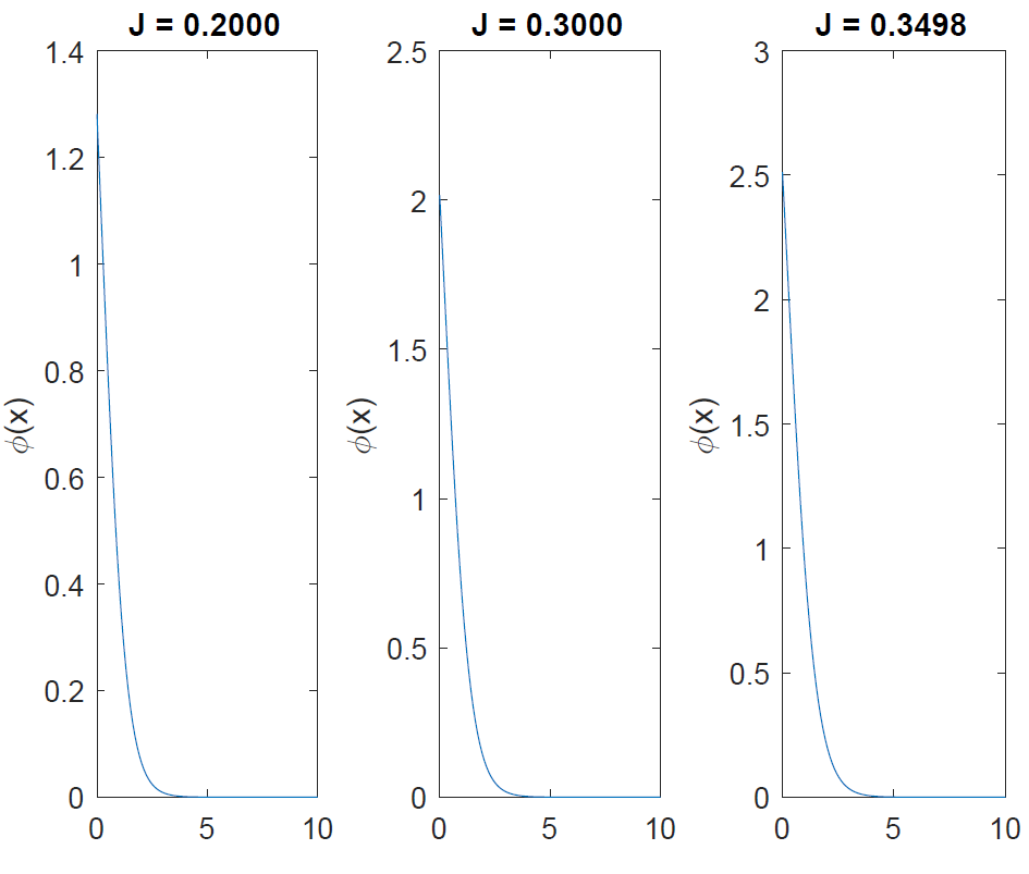
In this section we obtain the relation between the maximal current, for which a solution of (5) can exist, and $\sigma$ . To this end, we need to plot the solution $(\rho,\phi)$ of (5). A typical plot of $\rho(x)$ is provided in Fig. 1 for multiple values of J and $\sigma=.2$ .

Refer to caption — Figure 1: Graph of $\rho$ (x) in (5) for $\sigma$ = .2. The left two graphs asymptotically match (5) as $x\to\infty$ . If $J>.35$ the graph becomes nonphysical.

Similarly, Fig. 2 presents a plot of $\phi$ (x) for the same values, as in Fig. 1, of $J$ and $\sigma$ .

We use MATLAB routine BV4PC to obtain the solution of (5). To this end we must first change it to a system of first order ODEs.


	$\displaystyle f_{1}=$	$\displaystyle\;\rho^{\prime}$	(6a)
	$\displaystyle f_{2}=$	$\displaystyle\;\frac{(\sigma\phi+J)^{2}}{\rho^{3}}-\rho(1-\rho^{2})$	(6b)
	$\displaystyle f_{3}=$	$\displaystyle\;\phi^{\prime}$	(6c)
	$\displaystyle f_{4}=$	$\displaystyle\;\frac{\rho^{2}\phi}{\sigma}$	(6d)
with boundary conditions at $x=0$ and $x=b$ for some constant $b\gg 1$ .

	$\displaystyle\rho(0)=$	$\displaystyle\;0$	(6e)
	$\displaystyle\rho(b)=$	$\displaystyle\;\rho_{\infty}$	(6f)
	$\displaystyle\phi(b)=$	$\displaystyle\;0$	(6g)
	$\displaystyle\phi^{\prime}(0)=$	$\displaystyle\;-\frac{J}{\sigma}$	(6h)

Clearly, any change in the values of $J$ and $\sigma$ will produce a change in $(\rho,\phi)$ . To determine the maximal value of $J$ , for which a solution of (5) can exist for a given $\sigma$ , we increase $J$ incrementally over a set of evenly spaced numbers $0=J_{0}<J_{1}<\ldots<J_{400}=J_{c}=\sqrt{\frac{4}{27}}$ (clearly, $J_{k}=kJ_{c}/400$ ). For each $J_{k}$ we graphed $\rho(x)$ . The smallest value of $J$ for which $\rho$ does not tend asymptotically to $\rho_{\infty}$ (i.e. $\rho(x)$ is nonphysical), should be close to the maximal current the wire can carry. (See Figure 1 for plots of physical solutions.) We denote this critical value by $J^{c}(\sigma)=\sup S(\sigma)$ .

3 Asymptotic Expansion

We begin by repeating the formal asymptotic expansion, as $\sigma\to 0$ , of $J^{c}(\sigma)$ from [2]. We then compare it with the numerical solution described in the previous section.

Since (5b) is a Schrödinger equation with potential given by $\rho^{2}/\sigma$ , it follows, in view of (5d), that any bounded solution decays exponentially fast as $x\to\infty$ . In the limit $\sigma\to 0$ we expect the decay to take place on a fast scale. As $\rho(0)=0$ , it makes sense to assume that $\rho\sim\alpha x$ in the close vicinity of $x=0$ , where $\alpha=\rho^{\prime}(0).$ Note that by Lemma 2.1 in [2], $|\rho^{\prime}|\leq\sqrt{\frac{2}{3}}$ and hence $\alpha$ must be bounded as $\sigma\to 0$ . The problem for $\phi$ (5b,e,f) then takes the form


$\displaystyle-\sigma$	$\displaystyle\phi^{\prime\prime}+\alpha^{2}x^{2}\phi=0$	$\displaystyle\text{in}\;\mathbb{R}_{+}$	(7a)
	$\displaystyle\phi^{\prime}(0)=-\frac{J}{\sigma}$	$\displaystyle\phi\ \xrightarrow[x\to\infty]{}0\,.$	(7b)

Consider the scaled coordinate $\xi=\alpha^{\frac{1}{2}}\sigma^{-{\frac{1}{4}}}x$ and the function

\Phi(\xi)=\frac{\alpha^{\frac{1}{2}}\sigma^{\frac{3}{4}}}{J}\phi(x).

The scaled form of (7) is


$\displaystyle-$	$\displaystyle\Phi^{\prime\prime}+\xi^{2}\Phi=\;0$	$\displaystyle\text{in}\;\mathbb{R}_{+}$	(8a)
	$\displaystyle\Phi^{\prime}(0)=\;-1$	$\displaystyle\quad\Phi\xrightarrow[\xi\to\infty]{}0\,.$	(8b)

We next attempt to obtain $\alpha$ which is a priory unknown. Let

H=\frac{1}{2}\Big[|\rho^{\prime}|^{2}+\frac{(\sigma\phi^{\prime}+J)^{2}}{\rho^{2}}+\rho^{2}-\frac{1}{2}\rho^{4}\Big]\,.

(9)

Differentiating (9) we obtain, with the aid of (5a) and (5b), that

H^{\prime}=(\sigma\phi^{\prime}+J)\phi\,.

Note that the above relation is exact as it follows from (5). Since we can precisely evaluate $H(0)$ and $H(\infty)$ in terms of $\rho_{\infty}$ and $\alpha$ it makes sense to approximate $H^{\prime}$ with the aid of (8), and then to use the approximation to obtain an estimate of $H(\infty)-H(0)$ . Upon comparison with the exact expression we shall be able to obtain an equation for $\alpha$ . Thus, integrating $H^{\prime}$ between $0$ and $\infty$ yields, by (4), (5c-f), and (9)

\int_{0}^{\infty}(\sigma\phi^{\prime}+J)\phi\,dx=\frac{J^{2}}{\alpha\sigma^{1/2}}\int_{0}^{\infty}(\Phi^{\prime}+1)\Phi\,d\xi=\rho_{\infty}^{2}-\frac{3}{4}\rho_{\infty}^{4}-\frac{1}{2}\alpha^{2}\,.

Define

A=2\int_{0}^{\infty}(\Phi^{\prime}+1)\Phi\,d\xi\,,

and rewrite the above equality as

\frac{AJ^{2}}{\alpha\sigma^{1/2}}=2\rho_{\infty}^{2}-\frac{3}{2}\rho_{\infty}^{4}-\alpha^{2}.

Since the right-hand side is bounded from above by $2$ , $J$ must tend to $0$ as $\sigma\to 0$ . Consequently, we must have by (4) that either $\rho_{\infty}\sim 1$ or $\rho_{\infty}\sim 0$ . Since, as stated above, our interest is only in the case $\rho_{\infty}\sim 1$ , we reach the asymptotic identity

\alpha^{2}+\frac{AJ^{2}}{\alpha\sigma^{1/2}}=\frac{1}{2}\,.

We can now extract $J$ as a function of $\alpha$ , i.e.,

J^{2}=(\alpha-2\alpha^{3})\frac{\sigma^{1/2}}{2A}\,.

The maximum of the right-hand-side, with respect to $\alpha$ , is obtained for $\alpha=1/\sqrt{6}$ . Consequently, we can conclude that the maximal current the wire can carry is given by

J^{c}(\sigma)=\sqrt{\frac{2}{A}}\Big(\frac{1}{6}\Big)^{3/4}\sigma^{1/4}\,.

(10)

We now attempt to obtain $A$ , so we can compare (10), obtained in [2], to the numerical solution of (5). To this end we express $\Phi$ in terms of the parabolic cylinder function $\text{U}(0,\xi)$ . It can be easily verified that

A=-\Phi^{2}(0)+2\int_{0}^{\infty}\Phi\>d\xi

(11)

By [1, Chapter 19] we have $\Phi=C\cdot U(0,\sqrt{2}\xi)$ . To obtain $C$ we utilize (8b) and write

\Phi^{\prime}(0)=C\cdot\sqrt{2}U^{\prime}(0,0)=-1\,\implies C=\frac{-1}{\sqrt{2}U^{\prime}(0,0)},

And hence,

\Phi(\xi)=\frac{2^{-\frac{1}{4}}\Gamma(\frac{1}{4})}{\sqrt{2\pi}}U(0,\sqrt{2}\xi)\,.

(12)

We estimate $\phi(x)$ using [1, 19.3.1, 19.3.3-4] together with [1, 19.2.5-6] for $x\leq 7$ and [1, 19.8.1] for $x>7$ to obtain from (11)

A\approx 0.4336\,.

Then, we use (10) to obtain that

J^{c}(\sigma)\sim 0.5602\cdot\sigma^{\frac{1}{4}}\,.

(13)

For small $\sigma$ , the asymptotic curve of $J^{c}(\sigma)$ aligns with the critical J values found numerically, as can be viewed in Fig. 3

Note that the asymptotic approximation for $J^{c}(\sigma)$ begins to diverge from the numerical value at about $\sigma\approx 0.13$ . Such a divergence is expected since (13) cannot tend to $J_{c}$ as $\sigma\to\infty$ .

It was established in [2] that the potential drop for $J=J^{c}(\sigma)$ formally satisfies, as $\sigma\to 0$ ,

\phi^{c}(0,\sigma)\sim[3A\sigma]^{-\frac{1}{2}}\cdot\Phi(0)\approx 2.3861\cdot\sigma^{-\frac{1}{2}}\,.

(14)

In Fig. 4 we plot the numerical value of $\phi^{c}(\sigma)$ (the solid curve) and the asymptotic estimate given by (14).

Unlike the approximation for critical current, the asymptotic approximation for potential drop does not diverge from its numerical counterpart.

4 Concluding remarks

In the previous sections we have obtained, for a semi-infinite superconducting wire both the critical current at which superconductivity is destroyed, as well as the maximal potential drop the normal-superconducting interface can sustain. In the following we summarize our main findings.

1.

As $\sigma\to\infty$ the critical current tends to the asymptotic value $J_{c}=\sqrt{4/27}$ obtained in the absence of boundaries from (4). Accordingly, the potential drop over the interface tends to zero. We may conclude from here that in the large conductivity limit the normal-superconducting interface should not not have much effect on the main properties of the wire.
2.

As $\sigma\to 0$ the critical current $J_{c}(\sigma)$ diminishes like $\sigma^{1/4}$ whereas the potential drop diverges like $\sigma^{-1/2}$ . We may derive from here the highly intuitive conclusion that a superconductor of small normal conductivity is not very useful to the purpose of carrying strong currents with minimal loss of energy.
3.

The critical current is an increasing function of $\sigma$ . Hence the asymptotic value $\sqrt{4/27}$ is optimal.

Acknowledgements:
This research was supported by NSF Grant DMS-1613471.

References

[1] M. Abramowitz and I. A. Stegun, Handbook of Mathematical Functions, Dover, 1972.
[2] Y. Almog, The interface between the normal state and the fully superconducting state in the presence of an electric current, Commun. Contemp. Math., 14 (2012), pp. 1250026, 27.
[3] Y. Almog, L. Berlyand, D. Golovaty, and I. Shafrir, Existence and stability of superconducting solutions for the Ginzburg-Landau equations in the presence of weak electric currents, J. Math. Phys., 56 (2015), pp. 071502, 13.
[4] , Existence of superconducting solutions for a reduced $\{$ G $\}$ inzburg- $\{$ L $\}$ andau model in the presence of strong electric currents, arXiv preprint arXiv:1611.02732, (2016).
[5] J. Berger, Influence of the boundary conditions on the current flow pattern along a superconducting wire, Phys. Rev. B, 92 (2015), p. 064513.
[6] P. G. de Gennes and J. Prost, The Physics of Liquid Crystals, Clarendon Press, 2nd. ed., 1995.
[7] P. G. D. Gennes, Superconductivity of Metals and Alloys, Westview, 1966.
[8] B. I. Ivlev and N. B. Kopnin, Electric currents and resistive states in thin superconductors, Advances in Physics, 33 (1984), pp. 47–114.
[9] B. I. Ivlev, N. B. Kopnin, and L. A. Maslova, Stability of current-carrying states in narrow finite-length superconducting channels, Zh. Eksp. Teor. Fiz., 83 (1982), pp. 1533–1545.
[10] S. Kallush and J. Berger, Qualitative modifications and new dynamic phases in the phase diagram of one-dimensional superconducting wires driven with electric currents, Phys. Rev. B, 89 (2014), p. 214509.
[11] J. Rubinstein, P. Sternberg, and J. Kim, On the behavior of a superconducting wire subjected to a constant voltage difference, SIAM Journal on Applied Mathematics, 70 (2010), pp. 1739–1760.
[12] J. Rubinstein, P. Sternberg, and Q. Ma, Bifurcation diagram and pattern formation of phase slip centers in superconducting wires driven with electric currents, Physical Review Letters, 99 (2007).
[13] J. Rubinstein, P. Sternberg, and K. Zumbrun, The Resistive State in a Superconducting Wire: Bifurcation from the Normal State, Archive for Rational Mechanics and Analysis, 195 (2010), pp. 117–158.
[14] M. Tinkham, Introduction to superconductivity, McGraw-Hill, 1996.