Large Field Ranges from Aligned
and Misaligned Winding

Motivated by understanding field distances for fields with potentials, we are naturally led to looking at axions. This is because their potential is well-controlled due to a discrete shift symmetry. The axion version of the Weak Gravity Conjecture reads [3]

$$fS\lesssim q\,.$$

(2.1)

Here, and henceforth, we set the Planck mass to unity, $M_{p}=1$. Furthermore, $f$ is the axion decay constant, $S$ is the action of the instanton satisfying the inequality and $q$ is its charge. The action for a canonically normalised axion is periodic under a shift $2\pi f$. Let us furthermore denote by $2\pi\Pi$ the periodicity of the potential generated by the instanton. We then have

$$\Pi=\frac{f}{q}\,.$$

(2.2)

It is important to note that this can be different from the periodicity of the axion since it is possible to have $q\gg 1$.

Depending on the instanton(s) satisfying (2.1), one can distinguish different versions of the WGC. In particular, the Strong WGC [3] states that (2.1) is satisfied for the instanton with the smallest action $S$. In the controlled instanton regime $S\gtrsim 1$, (2.1) implies $f\lesssim q$ and hence $\Pi\lesssim 1$. Therefore, if the Strong WGC holds, the axion potential is dominated by an instanton contribution with sub-Planckian periodicity, ruling out, e.g., large-field inflation.⁴⁴ 4 This is true modulo the small-action loophole pointed out in [13] (see also [64]). Conversely, an axion with a parametrically large monotonic region in the potential parametrically violates the Strong WGC. Note, however, that the Strong WGC does not impose any restriction on $f$, and hence, for large enough $q$, the axion field range can still be super-Planckian.

This is to be contrasted with the Smallest Charge WGC [3], which states that (2.1) is satisfied for an instanton with $q=1$. In the regime $S\gtrsim 1$, this implies $f\lesssim 1$ and hence a small field range. The Smallest Charge WGC is thus much more restrictive than the Strong WGC.⁵⁵ 5 Another reason why, despite its name, the Strong WGC is less strong than the Smallest Charge WGC is that its 1-form version does not have any implications for the spectrum of the low-energy EFT. In particular, if only the Strong WGC holds, the inequality $m\lesssim qg$ [3] can be satisfied by states with arbitrarily large charges and, hence, arbitrarily large masses. A variant of the Smallest Charge WGC is the (Sub-)Lattice WGC [21, 65], where an instanton satisfying (2.1) exists for every site on the charge lattice or, more generally, on a sub-lattice with coarseness $q_{c}\geq 1$.⁶⁶ 6 See also the less restrictive Tower WGC [66], where the WGC is also satisfied by a large number of states but they do not necessarily occupy a sub-lattice in charge space. While an apparent counter-example [3] to the case $q_{c}=1$ was later shown to be incorrect [20], there are more recent counter-examples which indeed violate the Smallest Charge/Lattice WGC for $q_{c}=1$ [21, 65]. We stress, however, that it is an open problem whether the Sub-Lattice WGC is true for sub-lattices with $q_{c}>1$ (but still $\mathcal{O}(1)$). As we will see below, our type IIB constructions in Sect. 3 correspond to a parametric violation of this statement, i.e., to sub-lattices with parametrically large $q_{c}$. We will furthermore argue in Sect. 3 that it may be possible to construct axion potentials with large monotonic regions in our type IIB setting. According to our above discussion, this would correspond to a parametric violation of the Strong WGC.

We would like to test axion field distances and the related versions of the WGC directly in string theory. We are therefore interested in setups which lead to $f\gg 1$. The most reliable settings utilise constructions with two or more axions, in the spirit of [9] (see also [67, 68]). The idea is to give all but one combination of them a large mass and study the remaining light direction in the resulting effective theory. The key property of a setup with several axions is the possibility of winding trajectories for the light direction by turning on fluxes [10]. In the simple case of two axions, this winding can be achieved by considering a superpotential of the form

$$\mathcal{W}=w(Z)+f(Z)(n_{1}\,U_{1}+n_{2}\,U_{2})\,.$$

(2.3)

Here, $n_{1},n_{2}\in\mathbb{Z}$ are fluxes and $U_{1},U_{2}$ correspond to two distinguished complex-structure moduli. The remaining moduli are denoted by $Z$. The axions, $a_{1}$ and $a_{2}$, are the real parts of the $U_{i}$, while the saxions, $u_{1}$ and $u_{2}$, are the imaginary parts: $U_{i}=a_{i}+iu_{i}$. The associated decay constants are denoted by $f_{1}$ and $f_{2}$, where we assume $f_{1},f_{2}\lesssim 1$. The axions have associated instantons with actions $S_{1}=u_{1}$, $S_{2}=u_{2}$. Assuming that the instantons are unit-charged, we furthermore have $\Pi_{1}=f_{1}$ and $\Pi_{2}=f_{2}$.

The combination of axions which obtains a large mass from (2.3) is $n_{1}a_{1}+n_{2}a_{2}$. We are interested in the effective theory of the surviving light axion combination. To quantify the effective field range, it is useful to introduce the co-prime parts of $n_{1}$ and $n_{2}$, so we write

$$n_{1}=p\,p_{1}\,,\quad n_{2}=p\,p_{2}\,,\qquad\mathrm{for\;largest\;}p\in\mathbb{Z}\;\mathrm{such\;that\;}p_{1},p_{2}\in\mathbb{Z}\,.$$

(2.4)

The potential is invariant under any axion shift $(\Delta a_{1},\Delta a_{2})$ orthogonal to $(p_{1},p_{2})$. Hence, we can parametrise the flat direction by some field $\chi$ as

$$\left(\begin{array}[]{c}a_{1}\\ a_{2}\end{array}\right)=\left(\begin{array}[]{c}-p_{2}\\ p_{1}\end{array}\right)\,\chi\;.$$

(2.5)

Here, without loss of generality, we redefined the fundamental axions $a_{1}$, $a_{2}$ such that the line parametrised by $\chi$ goes through $(0,0)$. The vector on the right-hand side is the smallest integer vector pointing along the flat direction so that $\chi$ is $2\pi$-periodic. The canonically normalised field obtained from $\chi$ will be denoted by $\psi$. At leading order in the mass ratios of the heavy and light axion combinations, we can extract the effective decay constant for the light direction $\psi$ by treating the massive axion as constant in the kinetic terms. In the absence of kinetic mixing between $a_{1}$ and $a_{2}$, we then find

	$\displaystyle{\cal L}$	$\displaystyle=f_{1}^{2}\left(\partial a_{1}\right)^{2}+f_{2}^{2}\left(\partial a_{2}\right)^{2}+A\,\mathrm{e}^{-S_{1}}\,\cos(a_{1})+B\,\mathrm{e}^{-S_{2}}\,\cos(a_{2})$
		$\displaystyle\simeq\left(p_{2}^{2}f_{1}^{2}+p_{1}^{2}f_{2}^{2}\right)\left(\partial\chi\right)^{2}+A\,\mathrm{e}^{-S_{1}}\,\cos\left(p_{2}\,\chi\right)+B\,\mathrm{e}^{-S_{2}}\,\cos\left(p_{1}\,\chi\right)$
		$\displaystyle\equiv\left(\partial\psi\right)^{2}+A\,\mathrm{e}^{-S_{1}}\,\cos\left(\dfrac{\psi}{\Pi_{1}}\right)+B\,\mathrm{e}^{-S_{2}}\,\cos\left(\dfrac{\psi}{\Pi_{2}}\right)\,.$		(2.6)

Note that, in the first line, we only displayed the instanton-generated part of the potential for $a_{1}$, $a_{2}$ and assumed for simplicity that there are no relative phases in the arguments of the cosines. The periodicities of $\psi$ in the two instantons, associated to $a_{1}$ and $a_{2}$, are

$$\Pi_{1}=\frac{f}{p_{2}}\,,\quad\Pi_{2}=\frac{f}{p_{1}}\,,$$

(2.7)

where

$$f=\left(p_{1}^{2}f_{2}^{2}+p_{2}^{2}f_{1}^{2}\right)^{\frac{1}{2}}\,.$$

(2.8)

The field range is determined by the periodicity of the full action. This is equivalent to the periodicity under the two instanton terms appearing in (2.6), i.e., both terms must be periodic under a single axion shift. Since $p_{1}$ and $p_{2}$ are co-prime, the periodicity of $\psi$ is then $f$, and this sets the field range. Comparing with (2.2), we also see that the associated charges of the instantons are $p_{1}$ and $p_{2}$.

We can now distinguish, within this setting, two scenarios for obtaining a large field range for $\psi$. First, we consider aligned winding, i.e.,

$$p_{1}\sim{\cal O}\left(1\right)\,,\quad p_{2}\sim{\cal O}\left(N\right)\,,$$

(2.9)

for some $N\gg 1$. This is illustrated as the first case in Fig. 1. According to (2.7) and (2.8), it allows for $f\gg 1$ as well as $\Pi_{2}\gg 1$. The second condition may admit large monotonic regions in the potential and possibly even inflation. For this reason, the alignment scenario was originally proposed in [9]. As dicussed above, this implies a parametric violation of the Smallest Charge WGC and the Strong WGC. If the latter holds, the sub-Planckian instanton, with periodicity $\Pi_{1}$, dominates the super-Planckian one (i.e., $S_{2}>S_{1}$) such that the monotonic regions in the potential are small.

The other scenario we consider is misaligned winding where we take

$$p_{1}\sim{\cal O}\left(N\right)\,,\quad p_{2}\sim{\cal O}\left(N\right)$$

(2.10)

with $p_{1}\neq p_{2}$. This is illustrated as the second case in Fig. 1. Here, it is manifest that the periodicities in the instantons are not parametrically large (cf. (2.7) and (2.8)), and so it would not be useful for inflation. However, the axion field range $f$ is parametrically enhanced such that we still have $f\gg 1$. We will exploit both aligned and misaligned winding to realise large field ranges in type IIB string theory.⁷⁷ 7 More generally, one could also consider flux choices such as $p_{1}\sim\mathcal{O}(N)$, $p_{2}\sim\mathcal{O}(N^{2})$, which share some of the features of both aligned and misaligned winding. In particular, the present example allows $\Pi_{2}\gg 1$ as in aligned winding and yields $f\gg\Pi_{1},\Pi_{2}$ as in misaligned winding. We will not consider such flux configurations in the remainder of this paper as the cases (2.9) and (2.10) are sufficient for the points we wish to make.

Let us see how misaligned winding fits into the framework of the WGC. We assume that there are two instantons associated to $a_{1}$ and $a_{2}$ which satisfy the WGC, i.e., $S_{i}f_{i}\lesssim 1$. For simplicity, we furthermore take $f_{1}=f_{2}$ and $p_{1}\sim p_{2}\sim N$. It then follows with (2.8) that

$$fS_{i}\lesssim N\,,$$

(2.11)

i.e., the WGC is satisfied by instantons with parametrically large charges under the light axion $\psi$. To consider the low-charge instantons, we would need to take instantons wrapping cycles in a homology class which is a linear combination of the homology classes of the ’fundamental’ cycles associated to $u_{1}$ and $u_{2}$. But the instantons we considered are the lightest leading instantons, and so the instantons with lower charges have a larger action. For $f\sim\mathcal{O}(N)$, they will therefore not satisfy the WGC inequality. The setup therefore amounts to a parametric violation of the Smallest Charge WGC [3]. Within the context of the Sub-Lattice WGC [21, 65], it amounts to a sub-lattice with parametrically large coarseness, as discussed above.

Let us finally address the Swampland Distance Conjecture. Applied to the case of our axion $\chi$, the refined SDC states that a tower of states with exponentially light masses $m\sim\mathrm{e}^{-c\Delta\chi}$, $c>0$ should appear as we move a super-Planckian distance $\Delta\chi\gtrsim 1$ in the axion field direction. However, the energy scale of the axion potential we constructed is exponentially small compared to the mass scales of the other moduli. This means that the variation of $\chi$ cannot generate a large backreaction and, consequently, the (moduli-dependent) masses of any tower of states will stay approximately constant. We therefore conclude that no tower of light states can appear as we move along the axion potential, i.e., the above construction, if realisable in string theory, could provide a counter-example to the refined SDC.

We now consider the winding scenario in AdS solutions of type IIA string theory compactified on a Calabi-Yau orientifold [69].⁸⁸ 8 These solutions are only known in the smeared limit, i.e., they do not take into account the local backreaction of the O6-planes. We will proceed with the assumption that this does not modify the results significantly (see, e.g., [70, 71, 72, 73, 74, 75] for discussions of the smearing issue). The aim is to review the construction in an explicit string-theory example but also to discuss some problems in type IIA which we believe are not present in the type IIB models we will study in Sects. 3 and 4. We will use the conventions of [76] and focus on the specific example of the mirror-dual of $\mathbb{CP}^{4}_{(1,1,2,2,6)}[12]$, which was analysed in [61] and illustrates the relevant points. The effective four-dimensional ${\cal N}=1$ supergravity is specified by the following Kahler potential and superpotential:

	$\displaystyle\mathcal{K}$	$\displaystyle=-2\mathrm{log}\left[\sqrt{su_{1}}\left(u_{2}-\frac{2}{3}u_{1}\right)\right]+\mathcal{K}_{T}\left(T^{A}-\bar{T}^{A}\right)\,,$		(2.12)
	$\displaystyle\mathcal{W}$	$\displaystyle=-n_{0}S-n_{1}U_{1}-n_{2}U_{2}+\mathcal{W}_{T}\left(T^{A}\right)+A_{0}\left(T^{A}\right)\mathrm{e}^{iS}+A_{1}\left(T^{A}\right)\mathrm{e}^{iU_{1}}+A_{2}\left(T^{A}\right)\mathrm{e}^{iU_{2}}\,.$		(2.13)

Here, we introduced the complex-structure moduli $S=\sigma+is$, $U_{1}=a_{1}+iu_{1}$, $U_{2}=a_{2}+iu_{2}$. The Kahler moduli $T^{A}$ have the Kahler potential

$$\mathcal{K}_{T}\left(T^{A}-\bar{T}^{A}\right)=-\log\left(\dfrac{i}{6}k_{ABC}(T^{A}-\bar{T}^{A})(T^{B}-\bar{T}^{B})(T^{C}-\bar{T}^{C})\right)$$

(2.14)

and superpotential

$\displaystyle\mathcal{W}_{T}(T^{A})=\dfrac{f_{0}}{6}k_{ABC}T^{A}T^{B}T^{C}+\dfrac{1}{2}k_{ABC}\tilde{f}^{A}T^{B}T^{C}+f_{A}T^{A}+\tilde{f}_{0}\,,$

(2.15)

where $f_{0}$, $\tilde{f}^{A}$, $f_{A}$ and $\tilde{f}_{0}$ are quantised RR fluxes, see, e.g., [77]. We will ignore the stabilisation of the Kahler sector for the moment and come back to this point further below.

The terms linear in the complex-structure moduli in (2.13) are induced by NSNS fluxes, while the exponential terms are instanton-induced. Although we have written instanton contributions for the moduli $S$, $U_{1}$ and $U_{2}$ in (2.13), the question of whether those contributions are present is a difficult one, cf. [78] for a review. We will proceed with the assumption that they all contribute but will keep in mind that this may not be the case for specific examples.

Perturbatively, all saxions and one combination of the 3 axions $\sigma$, $a_{1}$ and $a_{2}$ are fixed.⁹⁹ 9 The stabilisation scheme in this example is therefore slightly different from the rest of this paper where we always stabilise all but one axion combination by fluxes. Non-perturbatively, all the axions gain a mass, but these masses can be exponentially different according to how the saxions $s$, $u_{1}$ and $u_{2}$ are fixed. In the vacuum, we have that [61]

$$\frac{s}{u_{1}}=\frac{3n_{1}+2n_{2}}{3n_{0}}\,,\qquad\frac{s}{u_{2}}=\frac{n_{2}\left(3n_{1}+2n_{2}\right)}{6n_{0}\left(n_{1}+n_{2}\right)}\,,\qquad\frac{u_{1}}{u_{2}}=\frac{n_{2}}{2\left(n_{1}+n_{2}\right)}\,.$$

(2.16)

We now consider a setting where $n_{0}\gtrsim n_{1},n_{2}$. This implies that $s\lesssim u_{1},u_{2}$. Of the three axions we therefore have two heavy combinations: $\sigma$ and $n_{0}\sigma+n_{1}a_{1}+n_{2}a_{2}$. The remaining (exponentially) light axion is orthogonal to both of these combinations. Since the metric on the field space factorises between $\sigma$ and the $a_{i}$, this light direction is purely in the $a_{1}$ and $a_{2}$ space and orthogonal to $n_{1}a_{1}+n_{2}a_{2}$.

We therefore arrive at a situation similar to the two-axion toy model in the previous section. The periodicities of the two instantons associated to $u_{1}$ and $u_{2}$ can be written as

$$\Pi_{1}=\frac{f}{p_{2}}\,,\qquad\Pi_{2}=\frac{f}{p_{1}}\,,\qquad f=\sqrt{\frac{3}{8}}\frac{p_{2}}{u_{1}}=\sqrt{\frac{3}{2}}\frac{p_{1}+p_{2}}{u_{2}}\,.$$

(2.17)

Here, as earlier, the $p_{i}$ are the co-prime factors in the $n_{i}$. We can now utilise this example to illustrate both aligned and misaligned winding. We see that aligned winding is realised for the choice

$$p_{1}\sim{\cal O}\left(1\right)\,,\;\;p_{2}\sim{\cal O}\left(N\right)\;\implies\;\Pi_{1}\sim\frac{1}{u_{1}}\,,\;\;\Pi_{2}\sim f\sim\frac{N}{u_{1}}$$

(2.18)

for $N\gg 1$, while, for misaligned winding, we have

$$p_{1}\sim{\cal O}\left(N\right)\,,\;\;p_{2}\sim{\cal O}\left(N\right)\;\implies\;\Pi_{1}\sim\Pi_{2}\sim\frac{1}{u_{1}}\,,\;\;f\sim\frac{N}{u_{1}}\,.$$

(2.19)

Note that, due to the requirement of tadpole cancellation, $N$ is bounded by the number of O6-planes and can therefore not be made arbitrarily large.

It appears from the above discussion that, assuming the $u_{i}$ are not too large, we can use winding to construct super-Planckian field ranges in this model. However, there are in fact several problems:

• •

  The example of aligned winding may at first appear to have parametrically large monotonic regions in the potential, associated to $\Pi_{2}$. However, it was observed in [61] that (2.16) implies $u_{2}\approx 2u_{1}$ for large $N$ and therefore the dominant instanton is the one associated to $\Pi_{1}$, which is not enhanced. This makes the above setup unsuitable for inflation (but does a priori not exclude that the model is still an example with parametrically large $f$).

• •

  A second, previously unnoticed problem is the backreaction of the Kahler moduli. In particular, in a controlled regime, they backreact on the vevs of the $u_{i}$ in such a way that the parametric enhancement of $f$ is cancelled. This can be seen by noting that the energy densities in the 10d action have to be small in string units $2\pi\sqrt{\alpha^{\prime}}=1$, i.e.,

  $$|H_{3}|^{2}\lesssim 1\,,\quad\mathrm{e}^{2\phi}|F_{p}|^{2}\lesssim 1\,,$$

  (2.20)

  where $\mathrm{e}^{\phi}=g_{s}$ is the 10d dilaton and the contractions are with the string-frame metric. This ensures that higher-derivative corrections to the effective action are suppressed.¹⁰¹⁰ 10 The dilaton factor in the second inequality is due to the usual definition of the RR fields with an extra power of $g_{s}$ (see, e.g., [69]). Consider now in particular the bound on the Romans mass, $\mathrm{e}^{2\phi}F_{0}^{2}\lesssim 1$. In terms of the 4d moduli, this becomes

  $$\frac{\mathcal{V}}{\sqrt{su_{1}}}\left(u_{2}-\frac{2}{3}u_{1}\right)^{-1}f_{0}^{2}\lesssim 1\,,$$

  (2.21)

  where $\mathcal{V}$ is the string-frame volume and $f_{0}=F_{0}$ in string units. This can be shown to follow from the usual definition of the complex-structure and Kahler moduli in type IIA [77, 69]. Solving the $F$-term constraints for $s$ and $u_{i}$, we furthermore find, at leading order in $N$,

  $$s\sim\frac{f_{0}\mathcal{V}}{n_{0}}\,,\quad u_{i}\sim\frac{f_{0}\mathcal{V}}{N}\,,$$

  (2.22)

  where we used that $\mathcal{W}\sim\text{Im}\mathcal{W}_{T}\sim f_{0}\mathcal{V}$ [69]. Using (2.22) in (2.21), we arrive at the condition

  $$\mathcal{V}\gtrsim N^{2}\,.$$

  (2.23)

  Replacing $\mathcal{V}$ in (2.22) by (2.23), we find

  $$u_{i}\gtrsim f_{0}N\,.$$

  (2.24)

  According to (2.18), (2.19), the effective axion decay constant for (mis-)aligned winding trajectories is $f\sim\frac{N}{u_{1}}$. Since $f_{0}$ is an integer, it follows that

  $$f\lesssim 1\,,$$

  (2.25)

  and therefore the field range is necessarily small in the controlled regime.

• •

  We also stress that, in type IIA models, our light-axion EFT always lives in deep AdS space. This may sound surprising since, in the limit of large $F_{4}$ flux, the AdS curvature is small compared to the KK scale [69]. We therefore have a genuinely four-dimensional low-energy EFT for all moduli in an approximate flat regime. However, one can also check that the AdS scale is always of the order of the saxion masses.¹¹¹¹ 11 Depending on the compactification, some of the saxions and/or axions can be tachyonic, with masses above the Breitenlohner-Freedman bound [69]. To be able to integrate out the saxions, one needs to go to a lower scale into the deep AdS regime. It is therefore not possible to take a limit where a large-$f$ axion lives in approximate Minkowski space.

It is not clear to us whether there could be other type IIA models in which some or all of these issues are ameliorated. Also note that we assumed above that $n_{0}\gtrsim n_{1},n_{2}$ in order to arrive at an EFT for a single light axion, cf. the discussion below (2.16). One can show that, without this assumption, the bound (2.25) is slightly relaxed to $f\lesssim\sqrt{N}/\sqrt{n_{0}}$. This is still smaller than the naive scaling $f\sim N$ but may at least allow a moderate enhancement $f\sim\sqrt{N}$ for small enough $n_{0}$. In order to verify this, one would have to study in more detail the EFT for the 2 axions orthogonal to the heavy combination $n_{0}\sigma+n_{1}a_{1}+n_{2}a_{2}$.

Notice further that the axions $a_{1}$, $a_{2}$ arising from the RR $3$-form do not suffer from loop corrections in type IIA. We emphasise this point because, as we will later see, loop corrections to the axion potential are a limiting factor in related type IIB models.

Nevertheless, we consider it more promising to study aligned and misaligned winding in type IIB string theory instead. As usual in type IIB, the stabilisation of the complex-structure moduli is approximately independent of the Kahler moduli due to a no-scale structure at tree-level, with only small corrections at sufficiently large volumes. The backreaction problem described above is therefore not expected to occur in such models. Indeed, we will discuss several candidate constructions in Sect. 3 which plausibly realise large field ranges using the winding idea. We will also see in Sect. 4 that, for sufficiently small $g_{s}$, the AdS scale is small compared to the moduli mass scale such that we have an approximate Minkowski situation.

As described in [10], winding can be achieved with a flux-induced superpotential [79] of the form (2.3),

$$\mathcal{W}=w(Z)+f(Z)(n_{1}\,U_{1}+n_{2}\,U_{2})\,.$$

(3.1)

Here, $U_{1}=a_{1}+iu_{1}$ and $U_{2}=a_{2}+iu_{2}$ are two distinguished complex-structure moduli. The remaining complex-structure moduli and the axio-dilaton are collectively denoted by the variable or set of variables $Z$. Without loss of generality, we assume that the fluxes $n_{1}$, $n_{2}$ are co-prime. Kahler moduli stabilisation will be ignored for the moment – it is discussed in Sect. 4.

It is essential that we assume the moduli $U_{1}$, $U_{2}$ to be stabilised at large complex structure (LCS), such that $u_{1},u_{2}\gg 1$. As a result, terms in the periods of the CY which involve factors $\mathrm{e}^{iU_{1}}$ and $\mathrm{e}^{iU_{2}}$ can be ignored. This justifies the ansatz (3.1). We are agnostic about the moduli $Z$ – they may or may not be at LCS. We will assume, however, that their values are such that the Kahler potential is still well-approximated by its leading term in the LCS expansion. For example, we want to avoid situations where terms like $i(U_{i}-\overline{U}_{i})(U_{j}-\overline{U}_{j})(Z-\overline{Z})\lesssim 1$ because we tuned $Z$ to achieve $|Z-\overline{Z}|\ll 1$.

With these assumptions, the complex-structure sector of the Kahler potential

$$\mathcal{K}\supset-\log\Big[\mathcal{A}(Z,\bar{Z},U_{1}-\bar{U}_{1},U_{2}-\bar{U}_{2})\Big]$$

(3.2)

is shift-symmetric in $a_{1}=\text{Re}(U_{1})$ and $a_{2}=\text{Re}(U_{2})$. These are our axion candidates. More explicitly, the function $\mathcal{A}$ has the structure [80, 81]

$$\mathcal{A}(Z,\bar{Z},U_{1}-\bar{U}_{1},U_{2}-\bar{U}_{2})=\mathcal{A}_{3}(Z-\bar{Z},U_{1}-\bar{U}_{1},U_{2}-\bar{U}_{2})+ic+g(Z,\bar{Z})\,,$$

(3.3)

which is best explained in the language of the mirror-dual 3-fold. In this language, $Z$ and $U_{i}$ are 2-cycle-related Kahler moduli and $g(Z,\bar{Z})$ encodes worldsheet instanton effects $\sim\exp(iZ)$. The perturbative (in the dual language) term, which dominates at LCS or large dual volume, is given by the cubic polynomial

$$\mathcal{A}_{3}(Z-\bar{Z},U_{1}-\bar{U}_{1},U_{2}-\bar{U}_{2})=\frac{i}{3!}\kappa_{ijk}(Y^{i}-\bar{Y}^{i})(Y^{j}-\bar{Y}^{j})(Y^{k}-\bar{Y}^{k})\,.$$

(3.4)

Here, $Y$ denotes both $Z$- and $U$-moduli. The $\kappa_{ijk}$ are dual intersection numbers and $c=-i\zeta(3)\chi(X_{3})/(4\pi^{3})$ with $\chi(X_{3})$ the Euler characteristic of the Calabi-Yau threefold $X_{3}$.

We now make a choice which is important for the following discussion: In the dual language, $Y^{i}$ are components of the Kahler form in a certain basis. We choose this basis to be a basis of the Kahler cone. As a result, the triple intersection numbers are non-negative integers, $\kappa_{ijk}\geq 0$, see, e.g., [82, 83].

The key point for the winding idea is that the superpotential (3.1) is independent of a certain linear combination of $U_{1}$ and $U_{2}$. Hence, the $F$-term conditions

$$D_{U_{1}}\mathcal{W}=n_{1}\,f(Z)+\mathcal{K}_{U_{1}}\mathcal{W}=0\,,\quad D_{U_{2}}\mathcal{W}=n_{2}\,f(Z)+\mathcal{K}_{U_{2}}\mathcal{W}=0$$

(3.5)

leave a flat direction on the $a_{1}$-$a_{2}$ field space. For $\mathcal{W}\neq 0$, these conditions can be rewritten as

	$\displaystyle\dfrac{\mathcal{K}_{U_{1}}}{\mathcal{K}_{U_{2}}}$	$\displaystyle=\dfrac{n_{1}}{n_{2}}\,,$		(3.6)
	$\displaystyle f(Z)+\dfrac{\mathcal{K}_{U_{1}}}{n_{1}}\mathcal{W}$	$\displaystyle=0\,.$		(3.7)

The first equation corresponds to fixing the relative volume of two (dual) $4$-cycles. Their overall volume is fixed by (3.7). This second equation also stabilises one linear combination of $a_{1}$ and $a_{2}$.

The plan is now to investigate properties of the field range $f$ of the surviving effective axion in the $a_{1}$-$a_{2}$-plane. This proceeds by analogy to the derivation of (2.8). First, recall the relevant kinetic terms,

$\displaystyle\mathcal{L}$

$\displaystyle\supset\mathcal{K}_{U_{1}\bar{U}_{1}}|\mathop{}\!\mathrm{\partial}U_{1}|^{2}+\mathcal{K}_{U_{1}\bar{U}_{2}}(\mathop{}\!\mathrm{\partial}U_{1})(\mathop{}\!\mathrm{\partial}\bar{U}_{2})+h.c.+\mathcal{K}_{U_{2}\bar{U}_{2}}|\mathop{}\!\mathrm{\partial}U_{2}|^{2}\;.$

(3.8)

Next, introduce the effective axion $\chi$ through $(a_{1},a_{2})\equiv(-n_{2},n_{1})\,\chi$, cf. (2.5). The decay constant of $\chi$ then reads

$$f^{2}=n_{2}^{2}\mathcal{K}_{U_{1}\bar{U}_{1}}-2n_{1}n_{2}\mathcal{K}_{U_{1}\bar{U}_{2}}+n_{1}^{2}\mathcal{K}_{U_{2}\bar{U}_{2}}\,.$$

(3.9)

To analyse this result, it will be convenient to think in terms of derivatives with respect to the real variables $u_{1}$ and $u_{2}$. For example, we have $4\mathcal{K}_{U_{1}\bar{U}_{2}}=\mathop{}\!\mathrm{\partial}_{u_{1}}\mathop{}\!\mathrm{\partial}_{u_{2}}\mathcal{K}$ and $4\mathcal{K}_{U_{2}}\mathcal{K}_{\bar{U}_{2}}=(\mathop{}\!\mathrm{\partial}_{u_{2}}\mathcal{K})^{2}$. To simplify notation, we will furthermore write $2\mathcal{K}_{2}\equiv\mathop{}\!\mathrm{\partial}_{u_{2}}\mathcal{K}$, $4\mathcal{K}_{12}\equiv\mathop{}\!\mathrm{\partial}_{u_{1}}\mathop{}\!\mathrm{\partial}_{u_{2}}\mathcal{K}$ etc.¹²¹² 12 Beware of the factor of $i$ appearing in the relation between, e.g., ${\cal K}_{1}$ and ${\cal K}_{U_{1}}$. With this, we have for example

$\displaystyle\mathcal{K}_{11}$

$\displaystyle=\mathcal{K}_{1}\mathcal{K}_{1}-\dfrac{\mathcal{A}_{11}}{\mathcal{A}}=\dfrac{n_{1}^{2}}{n_{2}^{2}}\mathcal{K}_{2}\mathcal{K}_{2}-\dfrac{\mathcal{A}_{11}}{\mathcal{A}}\,,$

(3.10)

where we used (3.6) in the second equality. Similar expressions can be given for $\mathcal{K}_{12}$ and $\mathcal{K}_{22}$. As a result, (3.9) simplifies to

$$f^{2}=-n_{2}^{2}\dfrac{\mathcal{A}_{11}}{\mathcal{A}}+2n_{1}n_{2}\dfrac{\mathcal{A}_{12}}{\mathcal{A}}-n_{1}^{2}\dfrac{\mathcal{A}_{22}}{\mathcal{A}}\,.$$

(3.11)

Note that, while not apparent in this form, $f^{2}$ continues to be positive definite. In other words, in any consistent model, the various quantities on the right-hand side of (3.11) will always take values which ensure positivity.

We would like to understand the properties of (3.11) in case of aligned or misaligned trajectories. Let us first consider the case of a small ratio in (3.6). We choose fluxes $(n_{1},n_{2})\rightarrow(1,N)$ with $N\gg 1$ corresponding to the setup investigated in [10]. Note that $N$ has to be positive because of (3.6) and $\mathcal{K}_{U_{1}}/\mathcal{K}_{U_{2}}>0$. In this case, since only $a_{1}+N\,a_{2}$ is stabilised, we obtain a winding trajectory closely aligned with $a_{1}$, hence the name aligned trajectory. The range of the $U_{1}$-axion is $N$-fold extended in this way. By (3.4), the function ${\cal A}$ is just a cubic polynomial in the imaginary parts of the $U_{i}$ with positive coefficients. Hence, its second derivatives are non-negative: $\mathcal{A}_{11},\mathcal{A}_{12},\mathcal{A}_{22}\geq 0$. Since $\mathcal{A}>0$, the first and last term in (3.11) contribute negatively. Thus, we estimate

$$f^{2}\leq 2N\dfrac{\mathcal{A}_{12}}{\mathcal{A}}\,.$$

(3.12)

We claim that this bound implies $f^{2}\ll 1$.

To demonstrate this, rewrite the inequality as

$\displaystyle f^{2}$

$\displaystyle\leq 2N\dfrac{u_{2}\mathcal{A}_{2}}{\mathcal{A}}\dfrac{\mathcal{A}_{12}}{u_{2}\mathcal{A}_{2}}=2N\dfrac{u_{2}\mathcal{A}_{2}}{\mathcal{A}}\dfrac{\mathcal{A}_{12}}{u_{2}N\mathcal{A}_{1}}\,,$

(3.13)

where we used (3.6) in the second step. Indeed, let us define the ratios

$\displaystyle E_{2}$

$\displaystyle\coloneqq\dfrac{\mathcal{A}}{u_{2}\mathcal{A}_{2}}\,,\qquad E_{12}\coloneqq\dfrac{\mathcal{A}_{1}}{u_{2}\mathcal{A}_{12}}\,.$

(3.14)

In terms of $E_{2}$ and $E_{12}$, Eq. (3.13) becomes

$$f^{2}\leq\dfrac{2}{u_{2}^{2}}\,\dfrac{1}{E_{2}E_{12}}\,.$$

(3.15)

It is clear that, whenever $\mathcal{A}$ is dominated by the perturbative term (3.4), we have $u_{2}{\cal A}_{2}\leq\mathcal{O}(1){\cal A}$. The reason is simple: If all terms in ${\cal A}$ involve $u_{2}$, then $u_{2}{\cal A}_{2}\sim{\cal A}$ ignoring ${\cal O}(1)$ factors. But ${\cal A}$ may involve terms without $u_{2}$. These are annihilated when taking the derivative, thus making $u_{2}{\cal A}_{2}$ generically smaller. Therefore, the ratio $E_{2}$ cannot become parametrically small: $E_{2}\gtrsim 1$. This also holds for $E_{12}$ so that $E_{12}\gtrsim 1$. Since $u_{2}\gg 1$ in the LCS limit, we deduce that $f^{2}\ll 1$. We formulate our observations in terms of a no-go theorem:

No-go theorem for aligned winding trajectories with two moduli: Consider a IIB flux compactification on a Calabi-Yau orientifold. Let two complex-structure moduli $U_{1}$, $U_{2}$ be at LCS with all others such that the perturbative terms in the Kahler potential dominate. If the superpotential $\mathcal{W}$ only depends on $U_{1}$, $U_{2}$ through the linear combination¹³¹³ 13 Note that the no-go theorem does not rely on the specific form of the superpotential in Eq. (3.1) but holds more generally for any $\mathcal{W}=\mathcal{W}(U_{1}+NU_{2},Z)$.$U_{1}+N\,U_{2}$ with $N\gg 1$, then the field range of the remaining flat axionic direction cannot become parametrically large.¹⁴¹⁴ 14 This no-go result does not apply to the toroidal examples of [42], which studied large field ranges in the regime $u_{i}\lesssim 1$. Due to the absence of instantons on the torus, this does not imply a loss of control.

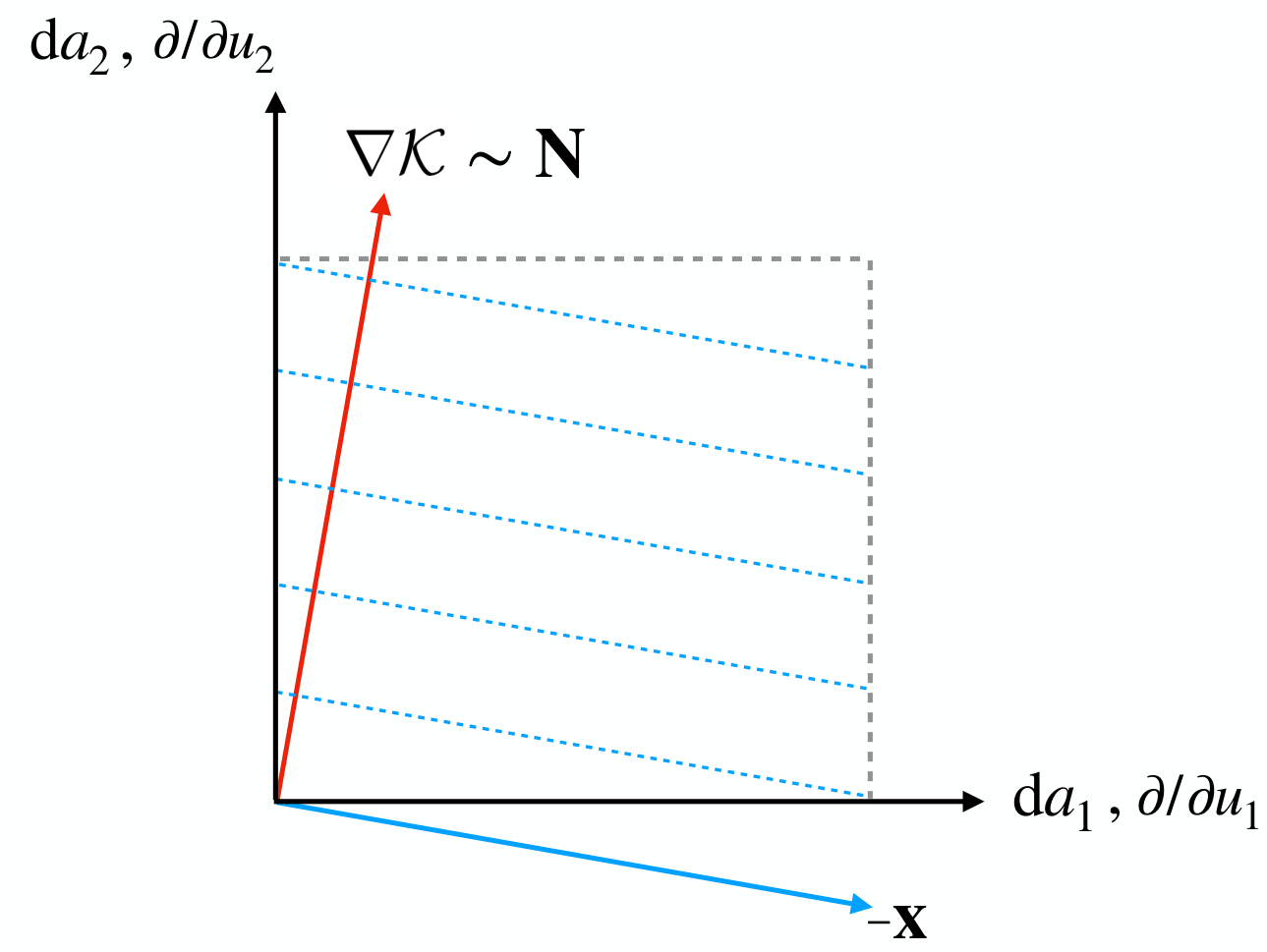
To understand this result intuitively, rewrite the $F$-term conditions (3.5) as

$$f(Z)\,\mathbf{N}-i\nabla\mathcal{K}\,W=0\,,$$

(3.16)

with

$$\mathbf{N}=\left(\begin{array}[]{c}n_{1}\\ n_{2}\end{array}\right)\,,\quad\nabla\mathcal{K}=\left(\begin{array}[]{c}\mathcal{K}_{1}\\ \mathcal{K}_{2}\end{array}\right)\,.$$

(3.17)

Furthermore, recall that we parametrise the light axion direction by $\chi$ as in Sect. 2.1 (see comment after (3.8)) and define a vector pointing into this direction,

$$\mathbf{x}=\frac{\text{d}\text{Re}(\mathbf{U})}{\text{d}\chi},\qquad\mathbf{U}=\left(\begin{array}[]{c}U_{1}\\ U_{2}\end{array}\right)\,.$$

(3.18)

Our intuitive argument is based on the arrangement of the three vectors $\mathbf{N}$, $\nabla\mathcal{K}$ and $\mathbf{x}$: On the one hand, $\nabla\mathcal{K}$ lives in the tangent space of the saxionic field space, with basis $(\partial/\partial u_{1},\partial/\partial u_{2})$. The vector $\mathbf{N}$ is parallel to $\nabla\mathcal{K}$ due to (3.16) and can be plotted in the same space, cf. Fig. 2. On the other hand, $\mathbf{x}$ lives in the cotangent space of the axionic field space, with basis $(\mathrm{d}a_{1},\mathrm{d}a_{2})$. It will be convenient to identify these two vector spaces using the above bases. In other words, we draw all vectors in a single space, see again Fig. 2. Orthogonality between two vectors from these two spaces becomes Euclidean orthogonality.

Now, the superpotential (3.1) forces the flat axionic direction to satisfy $n_{1}\mathrm{d}a_{1}+n_{2}\mathrm{d}a_{2}=0$. In other words, the flat direction is orthogonal to the flux vector $\mathbf{N}$:

$$\mathbf{N}\cdot\mathbf{x}=0\,.$$

(3.19)

Furthermore, $\nabla\mathcal{K}\sim\mathbf{N}$, such that the direction of $\nabla\mathcal{K}$ is fully determined by the light axion direction. In particular, aligning the light axion with the $a_{1}$-axis implies that $\nabla\mathcal{K}$ is aligned with the $a_{2}$-axis, see Fig. 2. Because of $\nabla\mathcal{K}=(\mathcal{K}_{1},\mathcal{K}_{2})\sim(\mathcal{A}_{1},\mathcal{A}_{2})$, this implies a large hierarchy $|\mathcal{A}_{1}|\ll|\mathcal{A}_{2}|$, which with (3.4) translates into a hierarchy between (combinations of) saxion vevs. This hierarchy makes $f$ small.

To summarise, as we align $\chi$ with one of the fundamental axions, we are constrained to a special region in moduli space with a large hierarchy between the components of $\nabla\mathcal{K}$. In that region, also the second-derivative matrix of $\mathcal{K}$ is non-generic and, as shown by our no-go theorem, it counteracts the naive field-range extension due to $N\gg 1$. In the following, we will discuss possibilities to extend the field range by fluxes without being forced in such a special corner of moduli space (i.e., without the imposition of large hierarchies on the components of $\nabla\mathcal{K}$). In this context, the geometric point of view introduced here will be very useful.

The winding trajectory discussed in the previous subsection was closely aligned with the $a_{1}$-axis. As discussed in Sect. 2.1, we can also think of different kinds of alignment, for example, with the diagonal direction $\mathrm{d}a_{1}-\mathrm{d}a_{2}$ (cf. Fig. 3). In this sense, the flat direction is misaligned with the original axions $a_{1}$, $a_{2}$. This can be achieved by the flux choice $(n_{1},n_{2})=(N,N+1)$ with $N\gg 1$. The $F$-term constraint (3.6) then becomes

$$\dfrac{\mathcal{K}_{U_{1}}}{\mathcal{K}_{U_{2}}}=\dfrac{\mathcal{A}_{U_{1}}}{\mathcal{A}_{U_{2}}}=\dfrac{N}{N+1}\sim\mathcal{O}(1)\,.$$

(3.20)

Contrary to the alignment scenario, this does not impose a large hierarchy between moduli vevs. Repeating the steps after (3.11) for the flux choice $(n_{1},n_{2})=(N,N+1)$, we furthermore find that the bound on the axion decay constant is relaxed,

$$f^{2}\leq 2\,N(N+1)\dfrac{\mathcal{A}_{12}}{\mathcal{A}}=\frac{2}{u_{2}^{2}}\frac{N^{2}}{E_{2}E_{12}}\,.$$

(3.21)

The key point here is the enhancement factor $N^{2}$ relative to the aligned case of (3.15). This evades the no-go theorem.

As in the aligned case, a roughly $N$-fold enhancement of the axion periodicity arises from the winding around the torus of the original field space. However, in contrast to the aligned case, this enhancement is not counteracted by a hierarchy between moduli vevs and, hence, between $\mathcal{A}_{i}$ and $\mathcal{A}_{ij}$ factors.

The corresponding geometry is illustrated in Fig. 3: As $\mathbf{x}$ is aligned with one diagonal in the axion field space, $\nabla\mathcal{K}\sim\mathbf{N}$ must be aligned with the opposite diagonal in the saxionic tangent space (cf. (3.19)). Thus, we immediately see that there is no hierarchy between the components of $\nabla\mathcal{K}$. As explained above, we believe that this is the underlying reason allowing for long trajectories.

Our no-go theorem of Sect. 3.1 excludes aligned trans-Planckian trajectories in two-axion models. A key assumption in its derivation was the use of a purely perturbative (in the mirror-dual language) Kahler and superpotential with respect to the moduli $U_{1}$ and $U_{2}$. Thus, a natural way out might be to generalise our superpotential (3.1) by including instanton terms:

$$\mathcal{W}=w(Z)+f(Z)(n_{1}\,U_{1}+n_{2}\,U_{2})+A_{1}(Z)\mathrm{e}^{iU_{1}}+A_{2}(Z)\mathrm{e}^{iU_{2}}\,.$$

(3.22)

The $F$-term constraints (3.6), (3.7) become

	$\displaystyle\dfrac{\mathcal{K}_{U_{1}}}{\mathcal{K}_{U_{2}}}$	$\displaystyle=\dfrac{n_{1}\,f(Z)+iA_{1}(Z)\mathrm{e}^{iU_{1}}}{n_{2}\,f(Z)+iA_{2}(Z)\mathrm{e}^{iU_{2}}}\,,$		(3.23)
	$\displaystyle f(Z)$	$\displaystyle=-i\frac{A_{1}(Z)\mathrm{e}^{iU_{1}}}{n_{1}}-\dfrac{\mathcal{K}_{U_{1}}}{n_{1}}\mathcal{W}\,.$		(3.24)

As in Sect. 3.1, we choose $(n_{1},n_{2})=(1,N)$ with $N\gg 1$ and assume $u_{1},u_{2}\gg 1$. The idea is now to tune the function $f(Z)$ to be very small, such that the exponentially suppressed instanton terms in (3.23) can compete with it. By (3.24), $\mathcal{W}$ and hence $w(Z)$ will then also be small. Thus, in spite of the hierarchy between $n_{1}$ and $n_{2}$, we can hope to arrange $\mathcal{K}_{U_{1}}/\mathcal{K}_{U_{2}}\sim\mathcal{O}(1)$. As argued above, a large hierarchy between the components of $\nabla\mathcal{K}$ was the key issue underlying our no-go result. This suggests that large field ranges can be realised in models with a fine-tuned superpotential.

A possible objection to this construction is that the key superpotential term $f(Z)(U_{1}+NU_{2})$, which is responsible for stabilising the axion combination $a_{1}+Na_{2}$, is tuned small. One might be concerned that the hierarchy between this stabilised field and the light axion $\chi$ will be lifted due to the tuning of $f(Z)$. Clearly, this would go against the spirit of the whole approach. However, we do not expect this to be a problem in general. Indeed, let us assume for notational simplicity that $Z$ stands for just one modulus and consider the corresponding $F$-term contribution to the scalar potential:

$$|D_{Z}\mathcal{W}|^{2}=|\partial_{Z}f(Z)|^{2}\,|U_{1}+NU_{2}|^{2}+\partial_{Z}f(Z)(U_{1}+NU_{2})\mathcal{K}^{Z\bar{Z}}\partial_{\bar{Z}}\bar{w}(\bar{Z})+c.c.+\ldots\,,$$

(3.25)

where we dismissed exponentially small terms and terms that do not depend on $U_{1}+NU_{2}$. In order that the flux-induced mass generated for $a_{1}+Na_{2}$ does not become small, it is mandatory that the tuning for $|f|\ll 1$ does not imply $|\partial_{Z}f|\ll 1$. While we cannot exclude obstructions due to the $F$-term constraints for the $Z$-moduli, generic flux choices do not imply $|\partial_{Z}f|\ll 1$: For example, if $f(Z)\equiv Z$ becomes small because we are stabilised near the locus $Z=0$ in moduli space, $\partial_{Z}f$ continues to be unity.

Another potential worry is that it may not be possible to arrange both $u_{1},u_{2}\gg 1$ and $f(Z)\ll 1$ in a given compactification. In particular, one might be concerned that the $F$-term constraints for the $Z$-moduli restrict the allowed on-shell values of $w(Z)$ and/or $f(Z)$ such that (3.24) cannot be solved with $u_{1},u_{2}\gg 1$. Indeed, this turns out to be the case in simple models (e.g., on the torus). However, we see a priori no reason why this should be a general issue. In particular, in compactifications with several $Z$-moduli, we expect to have enough tuning freedom to realise the above conditions.

To make this point clearer, we want to review the fine-tuning cost of the presented construction. As before, we are dealing with a flux superpotential $\mathcal{W}(Z,U_{1},U_{2})$ with $Z=\{Z_{1},\cdots,Z_{n}\}$. We have to make a flux choice ensuring the particular structure $\mathcal{W}\supset f(Z)(U_{1}+NU_{2})$. The remaining flux choice is used, as is standard in the type IIB landscape framework, to place ourselves at a particular locus in complex-structure moduli space. The well-known underlying idea is that, via the solution of the $F$-term equations, the flux discretuum is mapped to an (in general rather dense) discretuum of points in moduli space (see, e.g., [84]). In this discretuum, we have to choose a point with $u_{1},\,u_{2}\gg 1$ and $|f(Z)|\ll 1$. Only the last tuning is special to the present subsection. The smallness of $\mathcal{W}$ and of $w(Z)$ follows from the $F$-term equation (3.24) and the definition of $w$ in (3.22) and requires no further tuning.

So far, we have formulated a no-go theorem for aligned winding trajectories and discussed two loopholes in scenarios where two axions mix. A third way of evading our no-go theorem is to consider the mixing of more than two axions. Indeed, we find evidence that already the mixing of three axions is sufficient to allow for long trajectories. As we will see, this is nicely illustrated by our geometric picture developed earlier.

Consider the superpotential

$$\mathcal{W}=w(Z)+f_{1}(Z)(n_{1}\,U_{1}+n_{2}\,U_{2}+n_{3}\,U_{3})+f_{2}(Z)(m_{1}\,U_{1}+m_{2}\,U_{2}+m_{3}\,U_{3})$$

(3.26)

as a simple generalisation of (3.1). The Kahler potential is defined as in (3.2), (3.3) with the replacement $\mathcal{A}(Z,\bar{Z},U_{1}-\bar{U}_{1},U_{2}-\bar{U}_{2})\to\mathcal{A}(Z,\bar{Z},U_{1}-\bar{U}_{1},U_{2}-\bar{U}_{2},U_{3}-\bar{U}_{3})$. Our superpotential now only depends on two linear combinations of the three moduli $U_{i}=a_{i}+iu_{i}$. The Kahler potential involves just the imaginary parts $u_{i}$. Thus, our setup has one light axion, just as in the case with only two distinguished moduli $U_{1}$ and $U_{2}$.

The $F$-term conditions for the $U_{i}$ read

$\displaystyle D_{U_{i}}\mathcal{W}$

$\displaystyle=n_{i}f_{1}+m_{i}f_{2}+\mathcal{K}_{U_{i}}\mathcal{W}=0\qquad\forall\,i=1,2,3\;.$

(3.27)

For $\mathcal{W}\neq 0$, this fixes the ratios of Kahler potential derivatives according to

$\displaystyle\dfrac{\mathcal{K}_{U_{j}}}{\mathcal{K}_{U_{i}}}=\frac{\mathcal{A}_{U_{j}}}{\mathcal{A}_{U_{i}}}$

$\displaystyle=\dfrac{n_{j}f_{1}+m_{j}f_{2}}{n_{i}f_{1}+m_{i}f_{2}}\qquad\forall\,i,j=1,2,3\;.$

(3.28)

We need the kinetic term of the light axion obtained after integrating out the heavy axionic combinations $n_{i}a_{i}$, $m_{i}a_{i}$ as well as the saxions $u_{i}$. As before, we parametrise the light axionic direction by a field $\chi$:

$$\left(\begin{array}[]{c}a_{1}\\ a_{2}\\ a_{3}\end{array}\right)=\left(\begin{array}[]{c}x_{1}\\ x_{2}\\ x_{3}\end{array}\right)\chi\qquad\mbox{or}\qquad\mathbf{a}=\mathbf{x}\,\chi\,.$$

(3.29)

Here, $\mathbf{x}$ is the smallest integer vector orthogonal to the flux vectors $\mathbf{N}=(n_{1},n_{2},n_{3})^{T}$ and $\mathbf{M}=(m_{1},m_{2},m_{3})^{T}$. This ensures that the field $\chi$ is $2\pi$-periodic. Explicitly, we have

$$x_{1}=\frac{n_{3}m_{2}-n_{2}m_{3}}{x_{0}}\,,\quad x_{2}=\frac{n_{1}m_{3}-n_{3}m_{1}}{x_{0}}\,,\quad x_{3}=\frac{n_{2}m_{1}-n_{1}m_{2}}{x_{0}}$$

(3.30)

with

$$x_{0}=\text{gcd}\left(n_{3}m_{2}-n_{2}m_{3},n_{1}m_{3}-n_{3}m_{1},n_{2}m_{1}-n_{1}m_{2}\right)\,.$$

(3.31)

A calculation similar to that in Sect. 3.1 determines the axion decay constant

$\displaystyle f^{2}$

$\displaystyle=\dfrac{1}{\mathcal{A}}\biggl\{-2\mathcal{A}_{31}x_{1}x_{3}-2\mathcal{A}_{32}x_{2}x_{3}-2\mathcal{A}_{12}x_{1}x_{2}-\sum_{k=1}^{3}\,\mathcal{A}_{kk}x_{k}^{2}\biggl\}\,.$

(3.32)

The periodicities with respect to each of the three fundamental instantons are

$$\Pi_{1}=\dfrac{f}{x_{1}}\,,\quad\Pi_{2}=\dfrac{f}{x_{2}}\,,\quad\Pi_{3}=\dfrac{f}{x_{3}}\,.$$

(3.33)

Again, we observe that the diagonal terms $\sim\mathcal{A}_{kk}$ always contribute negatively to $f^{2}$. Therefore, we estimate

$\displaystyle f^{2}$

$\displaystyle\leq\dfrac{2}{\mathcal{A}}\biggl\{-\mathcal{A}_{31}x_{1}x_{3}-\mathcal{A}_{32}x_{2}x_{3}-\mathcal{A}_{12}x_{1}x_{2}\biggl\}\,.$

(3.34)

Of course, any physical configuration must lead to $f^{2}>0$. As in the two-axion case, this is not manifest in (3.32), (3.34) but is ensured by the consistency of the underlying model.

References

- [1] C. Vafa, The String landscape and the swampland, \hrefhttp://arxiv.org/abs/hep-th/0509212hep-th/0509212.
- [2] H. Ooguri and C. Vafa, On the Geometry of the String Landscape and the Swampland, Nucl. Phys. B766 (2007) 21–33, [\hrefhttp://arxiv.org/abs/hep-th/0605264hep-th/0605264].
- [3] N. Arkani-Hamed, L. Motl, A. Nicolis, and C. Vafa, The String landscape, black holes and gravity as the weakest force, JHEP 06 (2007) 060, [\hrefhttp://arxiv.org/abs/hep-th/0601001hep-th/0601001].
- [4] E. Silverstein and A. Westphal, Monodromy in the CMB: Gravity Waves and String Inflation, Phys. Rev. D78 (2008) 106003, [\hrefhttp://arxiv.org/abs/0803.3085arXiv:0803.3085].
- [5] L. McAllister, E. Silverstein, and A. Westphal, Gravity Waves and Linear Inflation from Axion Monodromy, Phys. Rev. D82 (2010) 046003, [\hrefhttp://arxiv.org/abs/0808.0706arXiv:0808.0706].
- [6] F. Marchesano, G. Shiu, and A. M. Uranga, F-term Axion Monodromy Inflation, JHEP 09 (2014) 184, [\hrefhttp://arxiv.org/abs/1404.3040arXiv:1404.3040].
- [7] R. Blumenhagen and E. Plauschinn, Towards Universal Axion Inflation and Reheating in String Theory, Phys. Lett. B736 (2014) 482–487, [\hrefhttp://arxiv.org/abs/1404.3542arXiv:1404.3542].
- [8] A. Hebecker, S. C. Kraus, and L. T. Witkowski, D7-Brane Chaotic Inflation, Phys. Lett. B737 (2014) 16–22, [\hrefhttp://arxiv.org/abs/1404.3711arXiv:1404.3711].
- [9] J. E. Kim, H. P. Nilles, and M. Peloso, Completing natural inflation, JCAP 0501 (2005) 005, [\hrefhttp://arxiv.org/abs/hep-ph/0409138hep-ph/0409138].
- [10] A. Hebecker, P. Mangat, F. Rompineve, and L. T. Witkowski, Winding out of the Swamp: Evading the Weak Gravity Conjecture with F-term Winding Inflation?, Phys. Lett. B748 (2015) 455–462, [\hrefhttp://arxiv.org/abs/1503.07912arXiv:1503.07912].
- [11] T. Rudelius, On the Possibility of Large Axion Moduli Spaces, JCAP 1504 (2015), no. 04 049, [\hrefhttp://arxiv.org/abs/1409.5793arXiv:1409.5793].
- [12] T. Rudelius, Constraints on Axion Inflation from the Weak Gravity Conjecture, JCAP 1509 (2015), no. 09 020, [\hrefhttp://arxiv.org/abs/1503.00795arXiv:1503.00795].
- [13] A. de la Fuente, P. Saraswat, and R. Sundrum, Natural Inflation and Quantum Gravity, Phys. Rev. Lett. 114 (2015), no. 15 151303, [\hrefhttp://arxiv.org/abs/1412.3457arXiv:1412.3457].
- [14] M. Montero, A. M. Uranga, and I. Valenzuela, Transplanckian axions!?, JHEP 08 (2015) 032, [\hrefhttp://arxiv.org/abs/1503.03886arXiv:1503.03886].
- [15] J. Brown, W. Cottrell, G. Shiu, and P. Soler, Fencing in the Swampland: Quantum Gravity Constraints on Large Field Inflation, JHEP 10 (2015) 023, [\hrefhttp://arxiv.org/abs/1503.04783arXiv:1503.04783].
- [16] J. Brown, W. Cottrell, G. Shiu, and P. Soler, On Axionic Field Ranges, Loopholes and the Weak Gravity Conjecture, JHEP 04 (2016) 017, [\hrefhttp://arxiv.org/abs/1504.00659arXiv:1504.00659].
- [17] T. C. Bachlechner, C. Long, and L. McAllister, Planckian Axions and the Weak Gravity Conjecture, JHEP 01 (2016) 091, [\hrefhttp://arxiv.org/abs/1503.07853arXiv:1503.07853].
- [18] D. Junghans, Large-Field Inflation with Multiple Axions and the Weak Gravity Conjecture, JHEP 02 (2016) 128, [\hrefhttp://arxiv.org/abs/1504.03566arXiv:1504.03566].
- [19] B. Heidenreich, M. Reece, and T. Rudelius, Weak Gravity Strongly Constrains Large-Field Axion Inflation, JHEP 12 (2015) 108, [\hrefhttp://arxiv.org/abs/1506.03447arXiv:1506.03447].
- [20] B. Heidenreich, M. Reece, and T. Rudelius, Sharpening the Weak Gravity Conjecture with Dimensional Reduction, JHEP 02 (2016) 140, [\hrefhttp://arxiv.org/abs/1509.06374arXiv:1509.06374].
- [21] B. Heidenreich, M. Reece, and T. Rudelius, Evidence for a Lattice Weak Gravity Conjecture, \hrefhttp://arxiv.org/abs/1606.08437arXiv:1606.08437.
- [22] L. E. Ibanez, M. Montero, A. Uranga, and I. Valenzuela, Relaxion Monodromy and the Weak Gravity Conjecture, JHEP 04 (2016) 020, [\hrefhttp://arxiv.org/abs/1512.00025arXiv:1512.00025].
- [23] K. Kooner, S. Parameswaran, and I. Zavala, Warping the Weak Gravity Conjecture, Phys. Lett. B759 (2016) 402–409, [\hrefhttp://arxiv.org/abs/1509.07049arXiv:1509.07049].
- [24] R. Kappl, H. P. Nilles, and M. W. Winkler, Modulated Natural Inflation, Phys. Lett. B753 (2016) 653–659, [\hrefhttp://arxiv.org/abs/1511.05560arXiv:1511.05560].
- [25] A. Hebecker, F. Rompineve, and A. Westphal, Axion Monodromy and the Weak Gravity Conjecture, JHEP 04 (2016) 157, [\hrefhttp://arxiv.org/abs/1512.03768arXiv:1512.03768].
- [26] A. Hebecker, P. Mangat, S. Theisen, and L. T. Witkowski, Can Gravitational Instantons Really Constrain Axion Inflation?, \hrefhttp://arxiv.org/abs/1607.06814arXiv:1607.06814.
- [27] A. Hebecker, P. Henkenjohann, and L. T. Witkowski, What is the Magnetic Weak Gravity Conjecture for Axions?, Fortsch. Phys. 65 (2017), no. 3-4 1700011, [\hrefhttp://arxiv.org/abs/1701.06553arXiv:1701.06553].
- [28] A. Hebecker and P. Soler, The Weak Gravity Conjecture and the Axionic Black Hole Paradox, JHEP 09 (2017) 036, [\hrefhttp://arxiv.org/abs/1702.06130arXiv:1702.06130].
- [29] E. Palti, The Weak Gravity Conjecture and Scalar Fields, JHEP 08 (2017) 034, [\hrefhttp://arxiv.org/abs/1705.04328arXiv:1705.04328].
- [30] D. Lust and E. Palti, Scalar Fields, Hierarchical UV/IR Mixing and The Weak Gravity Conjecture, JHEP 02 (2018) 040, [\hrefhttp://arxiv.org/abs/1709.01790arXiv:1709.01790].
- [31] D. Klaewer and E. Palti, Super-Planckian Spatial Field Variations and Quantum Gravity, \hrefhttp://arxiv.org/abs/1610.00010arXiv:1610.00010.
- [32] F. Baume and E. Palti, Backreacted Axion Field Ranges in String Theory, JHEP 08 (2016) 043, [\hrefhttp://arxiv.org/abs/1602.06517arXiv:1602.06517].
- [33] I. Valenzuela, Backreaction Issues in Axion Monodromy and Minkowski 4-forms, JHEP 06 (2017) 098, [\hrefhttp://arxiv.org/abs/1611.00394arXiv:1611.00394].
- [34] R. Blumenhagen, I. Valenzuela, and F. Wolf, The Swampland Conjecture and F-term Axion Monodromy Inflation, JHEP 07 (2017) 145, [\hrefhttp://arxiv.org/abs/1703.05776arXiv:1703.05776].
- [35] M. Cicoli, D. Ciupke, C. Mayrhofer, and P. Shukla, A Geometrical Upper Bound on the Inflaton Range, \hrefhttp://arxiv.org/abs/1801.05434arXiv:1801.05434.
- [36] T. W. Grimm, E. Palti, and I. Valenzuela, Infinite Distances in Field Space and Massless Towers of States, \hrefhttp://arxiv.org/abs/1802.08264arXiv:1802.08264.
- [37] B. Heidenreich, M. Reece, and T. Rudelius, Emergence and the Swampland Conjectures, \hrefhttp://arxiv.org/abs/1802.08698arXiv:1802.08698.
- [38] R. Blumenhagen, D. Kläwer, L. Schlechter, and F. Wolf, The Refined Swampland Distance Conjecture in Calabi-Yau Moduli Spaces, JHEP 06 (2018) 052, [\hrefhttp://arxiv.org/abs/1803.04989arXiv:1803.04989].
- [39] R. Blumenhagen, Large Field Inflation/Quintessence and the Refined Swampland Distance Conjecture, in 17th Hellenic School and Workshops on Elementary Particle Physics and Gravity (CORFU2017) Corfu, Greece, September 2-28, 2017, 2018. \hrefhttp://arxiv.org/abs/1804.10504arXiv:1804.10504.
- [40] M. Dias, J. Frazer, A. Retolaza, M. Scalisi, and A. Westphal, Pole N-flation, \hrefhttp://arxiv.org/abs/1805.02659arXiv:1805.02659.
- [41] T. W. Grimm, C. Li, and E. Palti, Infinite Distance Networks in Field Space and Charge Orbits, \hrefhttp://arxiv.org/abs/1811.02571arXiv:1811.02571.
- [42] A. Hebecker, P. Henkenjohann, and L. T. Witkowski, Flat Monodromies and a Moduli Space Size Conjecture, JHEP 12 (2017) 033, [\hrefhttp://arxiv.org/abs/1708.06761arXiv:1708.06761].
- [43] A. Landete and G. Shiu, Mass Hierarchies and Dynamical Field Range, \hrefhttp://arxiv.org/abs/1806.01874arXiv:1806.01874.
- [44] G. Dvali, Three-form gauging of axion symmetries and gravity, \hrefhttp://arxiv.org/abs/hep-th/0507215hep-th/0507215.
- [45] N. Kaloper and L. Sorbo, A Natural Framework for Chaotic Inflation, Phys. Rev. Lett. 102 (2009) 121301, [\hrefhttp://arxiv.org/abs/0811.1989arXiv:0811.1989].
- [46] N. Kaloper, A. Lawrence, and L. Sorbo, An Ignoble Approach to Large Field Inflation, JCAP 1103 (2011) 023, [\hrefhttp://arxiv.org/abs/1101.0026arXiv:1101.0026].
- [47] P. Saraswat, The Weak Gravity Conjecture and Effective Field Theory, \hrefhttp://arxiv.org/abs/1608.06951arXiv:1608.06951.
- [48] T. Kobayashi, A. Oikawa, and H. Otsuka, New potentials for string axion inflation, Phys. Rev. D93 (2016), no. 8 083508, [\hrefhttp://arxiv.org/abs/1510.08768arXiv:1510.08768].
- [49] N. Cabo Bizet, O. Loaiza-Brito, and I. Zavala, Mirror quintic vacua: hierarchies and inflation, JHEP 10 (2016) 082, [\hrefhttp://arxiv.org/abs/1605.03974arXiv:1605.03974].
- [50] R. Blumenhagen, D. Herschmann, and F. Wolf, String Moduli Stabilization at the Conifold, JHEP 08 (2016) 110, [\hrefhttp://arxiv.org/abs/1605.06299arXiv:1605.06299].
- [51] R. Blumenhagen, D. Herschmann, and F. Wolf, Challenges for Moduli Stabilization and String Cosmology near the Conifold, \hrefhttp://arxiv.org/abs/1704.04140arXiv:1704.04140. [PoSCORFU2016,104(2017)].
- [52] A. Hebecker, S. C. Kraus, D. Lust, S. Steinfurt, and T. Weigand, Fluxbrane Inflation, Nucl. Phys. B854 (2012) 509–551, [\hrefhttp://arxiv.org/abs/1104.5016arXiv:1104.5016].
- [53] A. Hebecker, S. C. Kraus, M. Kuntzler, D. Lust, and T. Weigand, Fluxbranes: Moduli Stabilisation and Inflation, JHEP 01 (2013) 095, [\hrefhttp://arxiv.org/abs/1207.2766arXiv:1207.2766].
- [54] M. Arends, A. Hebecker, K. Heimpel, S. C. Kraus, D. Lust, C. Mayrhofer, C. Schick, and T. Weigand, D7-Brane Moduli Space in Axion Monodromy and Fluxbrane Inflation, Fortsch. Phys. 62 (2014) 647–702, [\hrefhttp://arxiv.org/abs/1405.0283arXiv:1405.0283].
- [55] L. E. Ibanez, F. Marchesano, and I. Valenzuela, Higgs-otic Inflation and String Theory, JHEP 01 (2015) 128, [\hrefhttp://arxiv.org/abs/1411.5380arXiv:1411.5380].
- [56] F. Carta, F. Marchesano, W. Staessens, and G. Zoccarato, Open string multi-branched and Kähler potentials, JHEP 09 (2016) 062, [\hrefhttp://arxiv.org/abs/1606.00508arXiv:1606.00508].
- [57] A. Landete, F. Marchesano, G. Shiu, and G. Zoccarato, Flux Flattening in Axion Monodromy Inflation, JHEP 06 (2017) 071, [\hrefhttp://arxiv.org/abs/1703.09729arXiv:1703.09729].
- [58] M. Kim and L. McAllister, Monodromy Charge in D7-brane Inflation, \hrefhttp://arxiv.org/abs/1812.03532arXiv:1812.03532.
- [59] I. García-Etxebarria, T. W. Grimm, and I. Valenzuela, Special Points of Inflation in Flux Compactifications, Nucl. Phys. B899 (2015) 414–443, [\hrefhttp://arxiv.org/abs/1412.5537arXiv:1412.5537].
- [60] H. Abe, T. Kobayashi, and H. Otsuka, Natural inflation with and without modulations in type IIB string theory, JHEP 04 (2015) 160, [\hrefhttp://arxiv.org/abs/1411.4768arXiv:1411.4768].
- [61] E. Palti, On Natural Inflation and Moduli Stabilisation in String Theory, JHEP 10 (2015) 188, [\hrefhttp://arxiv.org/abs/1508.00009arXiv:1508.00009].
- [62] A. Hebecker, S. Leonhardt, J. Moritz, and A. Westphal, Thraxions: Ultralight Throat Axions, \hrefhttp://arxiv.org/abs/1812.03999arXiv:1812.03999.
- [63] G. Buratti, J. Calderon, and A. M. Uranga, Transplanckian Axion Monodromy !?, \hrefhttp://arxiv.org/abs/1812.05016arXiv:1812.05016.
- [64] A. Hebecker, T. Mikhail, and P. Soler, Euclidean wormholes, baby universes, and their impact on particle physics and cosmology, \hrefhttp://arxiv.org/abs/1807.00824arXiv:1807.00824.
- [65] M. Montero, G. Shiu, and P. Soler, The Weak Gravity Conjecture in three dimensions, JHEP 10 (2016) 159, [\hrefhttp://arxiv.org/abs/1606.08438arXiv:1606.08438].
- [66] S. Andriolo, D. Junghans, T. Noumi, and G. Shiu, A Tower Weak Gravity Conjecture from Infrared Consistency, \hrefhttp://arxiv.org/abs/1802.04287arXiv:1802.04287.
- [67] M. Berg, E. Pajer, and S. Sjors, Dante’s Inferno, Phys. Rev. D81 (2010) 103535, [\hrefhttp://arxiv.org/abs/0912.1341arXiv:0912.1341].
- [68] I. Ben-Dayan, F. G. Pedro, and A. Westphal, Hierarchical Axion Inflation, Phys. Rev. Lett. 113 (2014) 261301, [\hrefhttp://arxiv.org/abs/1404.7773arXiv:1404.7773].
- [69] O. DeWolfe, A. Giryavets, S. Kachru, and W. Taylor, Type IIA moduli stabilization, JHEP 07 (2005) 066, [\hrefhttp://arxiv.org/abs/hep-th/0505160hep-th/0505160].
- [70] B. S. Acharya, F. Benini, and R. Valandro, Fixing moduli in exact type IIA flux vacua, JHEP 02 (2007) 018, [\hrefhttp://arxiv.org/abs/hep-th/0607223hep-th/0607223].
- [71] M. R. Douglas and R. Kallosh, Compactification on negatively curved manifolds, JHEP 06 (2010) 004, [\hrefhttp://arxiv.org/abs/1001.4008arXiv:1001.4008].
- [72] J. Blaback, U. H. Danielsson, D. Junghans, T. Van Riet, T. Wrase, and M. Zagermann, Smeared versus localised sources in flux compactifications, JHEP 12 (2010) 043, [\hrefhttp://arxiv.org/abs/1009.1877arXiv:1009.1877].
- [73] F. Saracco and A. Tomasiello, Localized O6-plane solutions with Romans mass, JHEP 07 (2012) 077, [\hrefhttp://arxiv.org/abs/1201.5378arXiv:1201.5378].
- [74] J. McOrist and S. Sethi, M-theory and Type IIA Flux Compactifications, JHEP 12 (2012) 122, [\hrefhttp://arxiv.org/abs/1208.0261arXiv:1208.0261].
- [75] F. F. Gautason, M. Schillo, T. Van Riet, and M. Williams, Remarks on scale separation in flux vacua, JHEP 03 (2016) 061, [\hrefhttp://arxiv.org/abs/1512.00457arXiv:1512.00457].
- [76] E. Palti, G. Tasinato, and J. Ward, WEAKLY-coupled IIA Flux Compactifications, JHEP 06 (2008) 084, [\hrefhttp://arxiv.org/abs/0804.1248arXiv:0804.1248].
- [77] T. W. Grimm and J. Louis, The Effective action of type IIA Calabi-Yau orientifolds, Nucl. Phys. B718 (2005) 153–202, [\hrefhttp://arxiv.org/abs/hep-th/0412277hep-th/0412277].
- [78] R. Blumenhagen, M. Cvetic, S. Kachru, and T. Weigand, D-Brane Instantons in Type II Orientifolds, Ann. Rev. Nucl. Part. Sci. 59 (2009) 269–296, [\hrefhttp://arxiv.org/abs/0902.3251arXiv:0902.3251].
- [79] S. B. Giddings, S. Kachru, and J. Polchinski, Hierarchies from fluxes in string compactifications, Phys. Rev. D66 (2002) 106006, [\hrefhttp://arxiv.org/abs/hep-th/0105097hep-th/0105097].
- [80] S. Hosono, A. Klemm, and S. Theisen, Lectures on mirror symmetry, pp. 235–280. Springer Berlin Heidelberg, Berlin, Heidelberg, 1994.
- [81] Y. Honma and M. Manabe, Exact Kahler Potential for Calabi-Yau Fourfolds, JHEP 05 (2013) 102, [\hrefhttp://arxiv.org/abs/1302.3760arXiv:1302.3760].
- [82] F. Denef, Les Houches Lectures on Constructing String Vacua, Les Houches 87 (2008) 483–610, [\hrefhttp://arxiv.org/abs/0803.1194arXiv:0803.1194].
- [83] G. Curio, A. Klemm, D. Lust, and S. Theisen, On the vacuum structure of type II string compactifications on Calabi-Yau spaces with H fluxes, Nucl. Phys. B609 (2001) 3–45, [\hrefhttp://arxiv.org/abs/hep-th/0012213hep-th/0012213].
- [84] F. Denef and M. R. Douglas, Distributions of flux vacua, JHEP 05 (2004) 072, [\hrefhttp://arxiv.org/abs/hep-th/0404116hep-th/0404116].
- [85] S. Gukov, C. Vafa, and E. Witten, CFT’s from Calabi-Yau four folds, Nucl. Phys. B584 (2000) 69–108, [\hrefhttp://arxiv.org/abs/hep-th/9906070hep-th/9906070]. [Erratum: Nucl. Phys.B608,477(2001)].
- [86] M. Cicoli, D. Klevers, S. Krippendorf, C. Mayrhofer, F. Quevedo, and R. Valandro, Explicit de Sitter Flux Vacua for Global String Models with Chiral Matter, JHEP 05 (2014) 001, [\hrefhttp://arxiv.org/abs/1312.0014arXiv:1312.0014].
- [87] V. Balasubramanian, P. Berglund, J. P. Conlon, and F. Quevedo, Systematics of moduli stabilisation in Calabi-Yau flux compactifications, JHEP 03 (2005) 007, [\hrefhttp://arxiv.org/abs/hep-th/0502058hep-th/0502058].
- [88] J. P. Conlon, F. Quevedo, and K. Suruliz, Large-volume flux compactifications: Moduli spectrum and D3/D7 soft supersymmetry breaking, JHEP 08 (2005) 007, [\hrefhttp://arxiv.org/abs/hep-th/0505076hep-th/0505076].
- [89] M. Cicoli, M. Goodsell, and A. Ringwald, The type IIB string axiverse and its low-energy phenomenology, JHEP 10 (2012) 146, [\hrefhttp://arxiv.org/abs/1206.0819arXiv:1206.0819].
- [90] J. P. Conlon and F. Quevedo, Kahler moduli inflation, JHEP 01 (2006) 146, [\hrefhttp://arxiv.org/abs/hep-th/0509012hep-th/0509012].
- [91] S. Kachru, R. Kallosh, A. D. Linde, and S. P. Trivedi, De Sitter vacua in string theory, Phys. Rev. D68 (2003) 046005, [\hrefhttp://arxiv.org/abs/hep-th/0301240hep-th/0301240].
- [92] D. Baumann, A. Dymarsky, I. R. Klebanov, J. M. Maldacena, L. P. McAllister, and A. Murugan, On D3-brane Potentials in Compactifications with Fluxes and Wrapped D-branes, JHEP 11 (2006) 031, [\hrefhttp://arxiv.org/abs/hep-th/0607050hep-th/0607050].
- [93] M. Berg, M. Haack, and B. Kors, Loop corrections to volume moduli and inflation in string theory, Phys. Rev. D71 (2005) 026005, [\hrefhttp://arxiv.org/abs/hep-th/0404087hep-th/0404087].
- [94] M. Berg, M. Haack, and B. Kors, On the moduli dependence of nonperturbative superpotentials in brane inflation, in Themes in Unification. Proceedings: 10th International Symposium on particles, strings and cosmology, (PASCOS 2004), Pran Nath Festschrift. Part II: Boston, USA, August 18-19, 2004, 2004. \hrefhttp://arxiv.org/abs/hep-th/0409282hep-th/0409282.
- [95] M. Cicoli, J. P. Conlon, and F. Quevedo, General Analysis of LARGE Volume Scenarios with String Loop Moduli Stabilisation, JHEP 10 (2008) 105, [\hrefhttp://arxiv.org/abs/0805.1029arXiv:0805.1029].
- [96] M. Cicoli, M. Kreuzer, and C. Mayrhofer, Toric K3-Fibred Calabi-Yau Manifolds with del Pezzo Divisors for String Compactifications, JHEP 02 (2012) 002, [\hrefhttp://arxiv.org/abs/1107.0383arXiv:1107.0383].
- [97] T. W. Grimm and A. Klemm, U(1) Mediation of Flux Supersymmetry Breaking, JHEP 10 (2008) 077, [\hrefhttp://arxiv.org/abs/0805.3361arXiv:0805.3361].
- [98] G. von Gersdorff and A. Hebecker, Kähler corrections for the volume modulus of flux compactifications, Phys. Lett. B624 (2005) 270–274, [\hrefhttp://arxiv.org/abs/hep-th/0507131hep-th/0507131].
- [99] M. Berg, M. Haack, and B. Kors, On volume stabilization by quantum corrections, Phys. Rev. Lett. 96 (2006) 021601, [\hrefhttp://arxiv.org/abs/hep-th/0508171hep-th/0508171].
- [100] M. Berg, M. Haack, and B. Kors, String loop corrections to Kahler potentials in orientifolds, JHEP 11 (2005) 030, [\hrefhttp://arxiv.org/abs/hep-th/0508043hep-th/0508043].
- [101] M. Berg, M. Haack, and E. Pajer, Jumping Through Loops: On Soft Terms from Large Volume Compactifications, JHEP 09 (2007) 031, [\hrefhttp://arxiv.org/abs/0704.0737arXiv:0704.0737].
- [102] V. Kaplunovsky and J. Louis, Field dependent gauge couplings in locally supersymmetric effective quantum field theories, Nucl. Phys. B422 (1994) 57–124, [\hrefhttp://arxiv.org/abs/hep-th/9402005hep-th/9402005].
- [103] C. P. Burgess, J. P. Derendinger, F. Quevedo, and M. Quiros, On gaugino condensation with field dependent gauge couplings, Annals Phys. 250 (1996) 193–233, [\hrefhttp://arxiv.org/abs/hep-th/9505171hep-th/9505171].
- [104] D. Junghans and G. Shiu, Brane curvature corrections to the 1 type II/F-theory effective action, JHEP 03 (2015) 107, [\hrefhttp://arxiv.org/abs/1407.0019arXiv:1407.0019].
- [105] G. Curio and V. Spillner, On the modified KKLT procedure: A Case study for the P(11169) [18] model, Int. J. Mod. Phys. A22 (2007) 3463–3492, [\hrefhttp://arxiv.org/abs/hep-th/0606047hep-th/0606047].
- [106] M. Cicoli, J. P. Conlon, A. Maharana, and F. Quevedo, A Note on the Magnitude of the Flux Superpotential, JHEP 01 (2014) 027, [\hrefhttp://arxiv.org/abs/1310.6694arXiv:1310.6694].
- [107] A. Hebecker, P. Mangat, F. Rompineve, and L. T. Witkowski, Tuning and Backreaction in F-term Axion Monodromy Inflation, Nucl. Phys. B894 (2015) 456–495, [\hrefhttp://arxiv.org/abs/1411.2032arXiv:1411.2032].
- [108] W. Buchmuller, E. Dudas, L. Heurtier, A. Westphal, C. Wieck, and M. W. Winkler, Challenges for Large-Field Inflation and Moduli Stabilization, JHEP 04 (2015) 058, [\hrefhttp://arxiv.org/abs/1501.05812arXiv:1501.05812].