Chaotic Tides in Migrating Gas Giants: Forming Hot and Transient Warm Jupiters via High-Eccentricity Migration2018Chaotic Tides in Migrating Gas Giants: Forming Hot and Transient Warm Jupiters via High-Eccentricity Migration–References
Abstract
High-eccentricity migration is an important channel for the formation of hot Jupiters (HJs). In particular, Lidov-Kozai (LK) oscillations of orbital eccentricity/inclination induced by a distant planetary or stellar companion, combined with tidal friction, have been shown to produce HJs on Gyr timescales, provided that efficient tidal dissipation operates in the planet. We re-examine this scenario with the inclusion of dynamical tides. When the planet’s orbit is in a high-eccentricity phase, the tidal force from the star excites oscillatory f-modes and r-modes in the planet. For sufficiently large eccentricity and small pericentre distance, the mode can grow chaotically over multiple pericentre passages and eventually dissipate non-linearly, drawing energy from the orbit and rapidly shrinking the semi-major axis. We study the effect of such chaotic tides on the planet’s orbital evolution. We find that this pathway produces very eccentric () warm Jupiters (WJs) on short timescales (a few to 100 Myrs). These WJs efficiently circularize to become HJs due to their persistently small pericentre distances. Chaotic tides can also save some planets from tidal disruption by truncating the LK eccentricity oscillations, significantly increasing the HJ formation fraction for a range of planet masses and radii. Using a population synthesis calculation, we determine the characteristics of WJs and HJs produced in this scenario, including the final period distribution, orbital inclinations and stellar obliquities. Chaotic tides endow LK migration with several favorable features to explain observations of HJs. We expect that chaotic tides are also important in other flavours of high- migration.
Keywords:
hydrodynamics — planets and satellites: dynamical evolution and stability1 Introduction
Despite over two decades of observations, the origins of hot Jupiters (HJs, giant planets with orbital periods days) remain puzzling (see Dawson & Johnson 2018, for a review). The materials and conditions necessary to form such massive planets are not thought to exist so close to a protostar. Some have suggested that HJs could form in-situ when a protoplanet migrates inward and accumulates a gas envelope (Boley et al. 2016; Batygin et al. 2016). However, most theories propose that a fully formed gas giant migrated toward its host star either via interaction with the protoplanetary disk (Lin et al. 1996; Kley & Nelson 2012, e.g.) or through tidal decay and circularization of a high-eccentricity orbit, a process termed “high-eccentricity migration." Equally puzzling is the origin of warm Jupiters (WJs), giant planets with periods between about 10 days and 200 days. Although these close-in giant planets (HJs and WJs) represent a relatively small population of exoplanetary systems compared to the more abundant super-earths, their dynamical history can potentially shape the architecture of planetary systems.
High-eccentricity migration is an appealing avenue for HJ formation. In this scenario, a gas giant is excited into a highly eccentric orbit via interactions with other planets or with a distant stellar companion. Strong planet-planet scattering (Rasio & Ford 1996; Chatterjee et al. 2008; Jurić & Tremaine 2008), various forms of secular interactions (Wu & Lithwick 2011; Hamers & Portegies Zwart 2016; Petrovich 2015b), or a combination of both (Nagasawa et al. 2008; Beaugé & Nesvorný 2012), can produce very eccentric gas giants. An highly inclined stellar or planetary companion can excite “Lidov-Kozai” (LK) oscillations (Lidov 1962; Kozai 1962; Naoz 2016, for a review), pushing the eccentricity of the giant planet to near unity (Wu & Murray 2003; Fabrycky & Tremaine 2007; Naoz et al. 2012; Correia et al. 2012; Petrovich 2015a; Anderson et al. 2016). In all cases, the orbit circularizes and decays to a period of few days due to the tidal dissipation within the planet.
High-eccentricity migration can account for several puzzling characteristics of observed HJs. For instance, tidal orbital decay produces the observed pile-up of HJs at an orbital period of days (Santerne et al. 2016, e.g.), corresponding to semi-major axes of a few times the Roche radii of the planets. Lidov-Kozai migration driven by an inclined stellar/planetary companion can naturally generate significant “spin-orbit” misalignments between the rotation axis of the host star and the orbital angular momentum axis of the planet, as observed in many HJ systems (Hébrard et al. 2008; Narita et al. 2009; Winn et al. 2009; Triaud et al. 2010; Albrecht et al. 2012; Winn & Fabrycky 2015); the chaotic evolution of the stellar spin axis driven by the changing planetary orbit plays a dominant role in producing the observed stellar oblqiuities (Storch et al. 2014; Anderson et al. 2016; Storch et al. 2017). Other flavors of high- migration can also produce appreciable spin-orbit misalignments (Lithwick & Wu 2014; Petrovich 2015b; Teyssandier et al. 2018, e.g.). In addition, direct RV and AO-imaging searches have shown that a large fraction of HJs have external massive planet companions at 5-20 au or distant stellar companions (50-2000 au) (Knutson et al. 2014; Ngo et al. 2015; Wang et al. 2015; Bryan et al. 2016), suggesting that dynamical interactions play a role in HJ formation. Huang et al. 2016 showed that most HJs do not have any detectable neighbors (while half of WJs are closely flanked by small neighbors), again suggesting that a significant fraction of HJs may have formed through high- migration.
A significant uncertainty in any high- migration scenario is tidal dissipation in the planet. Regardless of how the planet attains its high eccentricity, efficient tidal dissipation is necessary in order to circularize the planet’s orbit and to bring it from a semi-major axis of several au’s to au. So far, almost all studies of high- migration have relied on the parameterized weak-friction theory of equilibrium tides (Alexander 1973; Hut 1981). In order achieve tidal circularization within Gyrs in high- migration scenarios, the giant planet generally should be more dissipative than Jupiter by more than an order of magnitude (Socrates et al. 2012; Petrovich 2015a; Anderson et al. 2016, e.g.).
In general, the response of a fluid body (such as a giant planet) to tidal perturbation involves the excitation of internal waves and modes at different frequencies (Ogilvie 2014, see, e.g.,). For a body in a sufficiently eccentric orbit, oscillatory modes excited at pericentre by the star’s tidal potential can grow chaotically in amplitude, rapidly draining energy from the orbit over multiple close passages (Mardling 1995a; Mardling 1995b). This effect is important for high-eccentricity migration because the same conditions that allow a planet to migrate quickly – small pericentre distance and large eccentricity – are those that result in chaotic tidal behaviour. Ivanov & Papaloizou 2004 first studied the possibility that chaotic dynamical tides could speed up the circularization of eccentric gas giants. They developed an iterative algebraic map to simply follow mode evolution over many orbits from one pericentre passage to the next. More recently, Vick & Lai 2018 used a similar map (generalized to include linear mode dampling) to quantify the various dynamical behaviours of the “mode + eccentric orbit” system (see also Section 2 below); they suggested that chaotic tides could quickly produce eccentric warm Jupiters (WJs), with a semi-major axis between 0.1 and 1 au, that efficiently circularize to HJs. Wu 2018 also studied the orbital evolution of a planet experiencing chaotic tides, and uncovered some of the key features of LK high- migration with chaotic tides – we will examine these features in more details in the later sections of this paper.
In this paper, we present a comprehensive study of high-eccentricity migration of giant planets, incorporating a detailed model of chaotic tidal evolution. We focus on migration via the LK effect with a stellar companion. Although this flavour of high- migration may only account for a fraction of the HJ population, it is most suitable for systematic study since the initial conditions (such as the orbital properties of the stellar perturber) are reasonably well-justified, and it serves as a benchmark for other high- migration scenarios. Indeed, several aspects of our results presented in this paper can be applied to other flavours of high- migration (see Teyssandier et al. 2018, which studies dynamical tides in the “secular chaos” scenario). Comparing to our previous study of LK migration with static tides (Anderson et al. 2016; Muñoz et al. 2016), we show that including chaotic tides leads to a number of “favorable” features for the formation of close-in giant planets: e.g., it naturally produces eccentric WJs on short timescales ( Myrs) and speeds up the formation of HJs; it generates a wider HJ period distribution; and it prevents some gas giants from undergoing tidal disruption, thereby increase the HJ formation fraction. Overall, chaotic tides make high- migration a more promising mechanism for producing HJs
The structure of the paper is as follows. In Section 2 we revisit the derivation of the iterative map for the evolution of planetary oscillation modes (dynamical tides), starting from hydrodynamical equations and including the effect of planetray rotation; we examine the different dynamical behaviours of the “modes + eccentric orbit” system and discuss the conditions for various modes in the planet to become chaotic. In Section 3 we describe our model for coupling LK oscillations with chaotic tides. Section 4 discusses the key features and signposts of LK migration with chaotic tides and includes a number of analytical results that characterize chaotic tidal migration. In Section 5 we present our population synthesis study for planets undergoing LK oscillations with chaotic tides. In Section 6 we give analytical calculations for the HJ formation and tidal disruption fractions from this migration mechanism and compare them with our numerical results. We conclude in Section 7 with a summary of results and discussion of their implications.
2 Chaotic Dynamical Tides in Giant Planets in Eccentric Orbits
Consider a planet (mass and radius ) in a highly eccentric orbit around a star (mass ). At each pericentre passage, the time-varying gravitational potential of the star excites oscillatory modes (e.g. f-modes and r-modes) in the planet. Over multiple pericentre passages, the orbit and the modes exchange energy and angular momentum. In general, this exchange can occur in either direction depending on the phase of the modes (Kochanek 1992; Mardling 1995a). Provided the oscillation amplitudes are sufficiently small, one can determine the dynamical behaviour of the system using linear hydrodynamics (Mardling 1995a; Mardling 1995b; Lai 1996; Kumar & Goodman 1996; Lai 1997, e.g.). However, following the evolution of the system over many orbits can be challenging because of the short timescale associated with the pericentre passage. Fortunately, when the orbit is eccentric enough, such that the mode and the orbital evolution mainly occur at pericentre, the full hydrodynamic solution of the “eccentric orbit + oscillation modes" system can be expressed as an iterative map (Ivanov & Papaloizou 2004; Vick & Lai 2018).
2.1 Hydrodynamics of Tidally Forced Oscillations & Iterative Map
In Vick & Lai 2018, we presented a simple iterative map to describe the long-term evolution of an “eccentric orbit + oscillation modes" system. Our map neglected the rotation of the planet and assumed that the change in the mode amplitude during each pericentre passage is constant throughout the orbital evolution. Giant planets can have substantial rotations, which affect their mode properties and introduce a few subtleties to the mapping. Also, during the long-term evolution of the planet’s orbit driven by an external companion (the Lidov-Kozai effect), the pericentre distance can change appreciably, which affects mode excitation. Here we present a general derivation of the iterative map from linear hydrodynamics, allowing for the planet to rotate and for the pericentre distance (and thus the change in mode amplitude at pericentre) to vary between passages.
The stellar gravitational potential that excites oscillations in the planet is given by
| (1) |
where is the position vector (in spherical coordinates) relative to the centre of mass of the planet (the azimuthal angle is measured in the rotating frame of the planet, and is the rotation rate of the planet11 1 We assume the spin axis of the planet is aligned with the orbital angular momentum axis throughout this paper.). In equation (1), is the time-varying separation between the star and planet, is the orbital true anomaly, and is a constant defined in Press & Teukolsky 1977. The dominant (quadrupole) terms have with .
The response of the planet to tidal forcing is described by the Lagrangian displacement, . A free oscillatory mode of frequency (in the rotating frame) has the form , where is the mode index. We expand in terms of the eigenmodes in the phase space (Schenk et al. 2002):
| (2) |
The linear fluid dynamics equations then reduce to a set of first-order differential equations (Lai & Wu 2006),
| (3) |
where
| (4) |
is the dimensionless tidal overlap integral (in units where ), and
| (5) |
Note that in the slow rotation limit, is simply the mode frequency for a non-rotating planet, . When , the first-order correction to the mode frequency due to rotation is (Unno et al. 1989, e.g.). In equations (3)-(5), the eigenmode is normalized according to
| (6) |
The general solution to equation (3) is
| (7) |
where
| (8) |
is the mode frequency in the inertial frame.
For a highly eccentric orbit, we can assume that any energy transfer between a mode and the orbit occurs at pericentre. We can then manipulate equation (7) into a discrete form by defining as the time at apocentre after the -th pericentre passage, i.e.
| (9) |
where is the orbital period after the -th pericentre passage. We also define
| (10) |
Physically, this is the real change in mode amplitude during the -th pericentre passage. Equation (7) becomes
| (11) |
We assume the initial condition Equation (11) can be rewritten in an iterative form:
| (12) |
We now define the mode amplitude in the inertial frame and shift the index to count pericentre passages using
| (13) |
Physically, is the mode amplitude just before the -th pericentre passage. Equation (12) then becomes
| (14) |
where . Equation (14) has a straight-forward physical interpretation: when the planet passes through pericentre (the -th passage), the mode amplitude changes by , and the orbital period changes to ; as the planet completes its orbit, the phase of the mode evolves due to the passage of time, and the complex mode amplitude gains a factor . Note that in general depends on the “current" parameters of the system. If the pericentre distance and the shape of the orbit near pericentre remain unchanged over many passages, is nearly constant from one passage to the next. In this case, equation (14) reduces to the result from Vick & Lai 2018 but without mode damping and with the phase evolution determined by the mode frequency in the inertial frame (Ivanov & Papaloizou 2004, see also).
The mode amplitude is directly related to the mode energy via
| (15) |
where the factor of 2 arises because a mode with given , and is physically identical to that with and — we treat them as the same mode. We define the dimensionless mode energy, , in units of the initial binary (planetary) orbital energy, (where is the semi-major axis), and define the re-normalized mode amplitude such that
| (16) |
The total energy transfer to modes in the -th passage is therefore
| (17) |
From energy conservation, the orbital energy () immediately after the -th passage is given by
| (18) |
and the corresponding orbital period is
| (19) |
where , and is the initial period.
Equations (14) and (17)-(19) complete the map. The required inputs are the initial mode energy, , and , the change in mode amplitude during each pericentre passage. This map accurately determines the evolution of the orbit and mode energies provided that the orbit is highly eccentric and the modes remain linear (i.e., the sum of the mode energies is much less than the binding energy of the planet).
The dimensionless change in mode amplitude during a pericentre passage (suppressing the subscript ‘k’), , depends on the orbital parameters (mainly the pericentre distance ) and the mode properties. It is related to the energy transfer by
| (20) |
Note that in general the energy transfer to mode in a pericentre passage depends on the amplitude and phase of “pre-existing" oscillations [see equation (17)]. In equation (20), refers to the energy transfer when the mode has zero amplitude prior to the pericentre passage — in Vick & Lai 2018, we term this “the first passage." The energy transfer for a parabolic encounter () was first derived by Press & Teukolsky 1977. This can be generalized to eccentric orbits and modified to include the effect of rotation (Lai 1997; Fuller & Lai 2012). For a pericentre distance , can be written as (keeping only the terms)
| (21) |
where is the ratio of and the tidal radius , i.e.
| (22) |
with , and is the pericentre orbital frequency
| (23) |
Note that , with . To avoid tidal disruption of the planet, we require (Guillochon et al. 2011)
| or | (24) |
The dimensionless function is given by
| (25) |
where is an overlap integral (see equation 4), and
| (26) |
In equation (26), all quantities are in units where so that is dimensionless.
To follow the evolution of the system over many orbits, it is useful to be able to compute (and thus ) efficiently. For the dominant prograde mode (), Lai 1997 derived an approximation for that is accurate to within 2% for and a few:
| (27) |
As shown in Vick & Lai 2018, when the mode has no initial energy, i.e. , the important quantity that determines the dynamical behaviour of the system is , where is the change in the initial orbital period () due to the energy transfer . From equation (21), we have
| (28) |
Physically, is the phase change in the mode due to energy transfer at pericentre when there is no “pre-existing" mode energy.
2.2 Planetary Oscillation Modes
| Model Type | Mode | ||||
|---|---|---|---|---|---|
| polytrope | f-mode | 0.56 | |||
| i-mode 1 () | 0.56 | 0.28 | 2.56 | ||
| i-mode 2 () | -1.1 | -0.55 | 0.9 | 0.01 | |
| polytrope | f-mode | 0.49 |

The gravitational potential of a star can excite many types of oscillation modes in the eccentric orbiting planet. Some of the modes will be more strongly excited than others and therefore more influential in long-term orbital evolution. The dominant modes are quadrupole, with . The modes are generally much less important because (equation 26) is small. In this paper, we adopt the convention , so a mode with () is prograde (retrograde) with respect to the rotation of the planet in the inertial frame. For the rest of this paper, we only consider modes with .
We adopt a simple giant planet model composed of a neutrally stratified fluid characterized by a polytrope equation of state (). Of the acoustic modes (with the restoring force being pressure), the f-mode (fundamental mode) has a frequency closest to the frequency of tidal forcing near pericentre, and the largest tidal overlap integral . Other acoustic modes (p-modes) have higher frequencies and smaller tidal overlaps, and are much less important than the f-mode for energy transfer. For a rotating planet, the stellar potential can also excite i-modes [i.e. inertial modes, with the restoring force being the Coriolis force; see Xu & Lai 2017 and references therein]. In a gas giant that has stratification, g-modes (driven by buoyancy) may also be excited (Fuller 2014). The presence of a large solid core also supports elastic modes which can “mix" with the f-mode (Fuller et al. 2014, e.g.). We do not consider such planet models in this paper because there are considerable uncertainties in the stratification and core size of giant planets (Guillot 2005, e.g.).
Table 1 lists the key properties of the f-modes and the first two inertial modes for the polytropic planet model. For comparison, the f-mode properties of the polytrope are also given. The f-modes are calculated using the slow-rotation approximation, which gives , and we find for both the and models. The i-mode result is from Xu & Lai 2017 (see their Table IV), based on calculations using a non-perturbative spectral code. Note that for , the mode frequencies in the rotating frame () and in the inertial frame () are related by .
To determine which of these modes produces the strongest dynamical tides, we calculate with equation (28) as a function of for each of the modes (see Fig. 1). For definiteness, we assume that the planet rotates at the pseudosynchronous rate given by the weak friction theory of equilibrium tides (Hut 1981, e.g.), i.e.
| (29) |
where is the mean motion of the planet and
| (30) | ||||
| (31) |
For , , and the mode frequency in the inertial frame, , is nearly independent of the orbital eccentricity. In this limit, also has negligible eccentricity dependence, and [see equation (28)]. The two panels of Fig. 1 shows that indeed increases with for all modes. We are most interested in systems where is sufficiently small such that (the criterion for chaotic mode growth; see Section 2.3). For such systems, it is clear that the f-mode is most strongly excited at pericentre passages. For the remainder of the paper, we focus on the prograde f-mode and neglect the contributions to energy transfer from other modes.
2.3 Conditions for Chaotic Tides

When the planetary orbit is sufficiently eccentric, the change in mode amplitude in a pericentre passage, (or equivalently the energy transfer in the “first" passage, , see equation 21), is constant over many pericentre passages.22 2 This requires that the pericentre distance is constant, which in turn requires that the fractional change in the orbital angular momentum, , remains small throughout orbital evolution. See equation (13) of Vick & Lai 2018. In this case, if the mode has negligible dissipation, the dynamical behaviour of the iterative map depends on , the initial mode energy , and (see equation 28), assuming that the initial mode energy is negligible (see Section 2.4). In particular, a system with greater than a critical value, , behaves very differently from systems with . The exact value of depends on the dimensionless orbital period, . On average, . The map exhibits three classes of behaviour (Vick & Lai 2018):
(i) When , the mode energy undergoes low-amplitude oscillations. A small amount of energy (of order ) is transferred back and forth between the mode and the orbit over multiple pericentre passages. An example of this behaviour is shown in the top panel of Fig. 2.
(ii) When and is close to an integer (i.e., when is an integer multiple of the orbital frequency, ), the mode energy exhibits larger-amplitude oscillations with a mean mode energy (see the middle panel of Fig. 2.)
(iii) When , the mode amplitude evolves chaotically and can grow to very large values of order the initial orbital energy ; meanwhile, the orbit experiences significant decay in the semi-major axis. The bottom panel of Fig. 2 provides an example. Note that in this example the binding energy of the planet is of order the initial orbital energy ( for an initial semi-major axis au). For such chaotic systems, the mode energy will eventually grow to values comparable to the binding energy of the planet, at which point the linear treatment is no longer appropriate and the mode will dissipate energy due to non-linear effects. We will discuss the implications of non-linear dissipation in later sections.
These three different behaviours can be characterized by the maximum mode energy that is attained over many pericentre passages. The examples in Fig. 2 demonstrate that the mode energy remains a small fraction of the initial orbital energy for non-chaotic evolution. However, when the system behaves chaotically, the maximum mode energy, , can be significant compared to .

In Fig. 3 we explore the boundary for chaotic behaviour in the plane by recording over orbits for different planet models with and (the stellar mass is fixed at ). The left and right panels of Fig. 3 assume that is the pseudosynchronous rate from equation (29) while the middle panel uses a constant value of . Small changes in do not have a large effect on the chaotic boundary. The right panel of Fig. 3 uses a polytropic planet model rather than our standard choice of . A comparison between the right panel and others suggests that changes in the structure of the planet can significantly shift the boundary for chaotic behaviour.
Figure 3 demonstrates that the condition generally captures the boundary for chaotic behaviour. This boundary is somewhat fuzzy because the precise value of spans a wide range, from to , depending on the value of (Vick & Lai 2018, see Fig. 1 of). In particular, when is close to an integer (resonance). Figure 3 confirms that on average. When the change in the mode phase is nearly a random number mod , and each pericentre “kick" to the mode occurs at a random phase. Under this condition, the mode energy grows in a diffusive manner (Mardling 1995a; Ivanov & Papaloizou 2004; Wu 2018). Note that this “diffusion" is approximate; as explained in Vick & Lai 2018 (see their Fig. 3), there exists an upper limit to the mode energy even in the absence of dissipation. For this reason, we prefer to call the mode growth and dissipation in the regime “chaotic tides."
From equation (28), we see that is larger for more eccentric orbits, and smaller (i.e. smaller and larger ). A young gas giant that is pumped into a highly eccentric orbit can satisfy the condition for chaotic tidal evolution (see Fig. 3) and rapidly transfer orbital energy to the f-mode. This behaviour is most likely to occur for . The critical condition for chaotic tides, , can be written (using equation 28) as
| (32) |
Note that depends on and and is nearly independent of for large eccentricities. Equation (32) gives the critical eccentricity, for a given , above which chaotic tides operate as a function of the dimensionless pericentre distance (equation 22).33 3 The mode frequency depends on the planet rotation rate , which may depend on if the equilibrium rotation rate depends on . For pseudosynchronous rotation, this dependence is very weak when (for which ); see equation (29). If we make further simplification for the function by replacing in equation (25) with the approximate fitting formula (Wu 2018), equation (32) can be inverted to yield
| (33) |
or equivalently,
| (34) |
Equation (34) gives the critical pericentre distance for chaotic tides to operate as a function of eccentricity.
2.4 Conditions for Chaotic Tides When


In Section 2.3, we have discussed the condition for the onset of chaotic mode growth for an “eccentric orbit + oscillatory modes" system where there is no initial energy in the mode (). When dynamical tides are the only influence on the planet’s orbital evolution, and when the total energy of the system is conserved (i.e. the modes do not dissipate), and completely determine the behaviour of the system. For instance, a system with will never undergo chaotic mode growth, and one with will always be chaotic. However, when non-tidal effects alter the planet’s orbit (e.g. LK eccentricity oscillations driven by an external companion), a system can transition in and out of the chaotic regime as is driven below and above [see equations (32)-(34) and Fig. 3]. Therefore, it is useful to know whether a system is “currently chaotic" when there is “pre-existing" energy in the mode (). Here, we generalize the criterion for the onset of chaotic tides to account for the “pre-existing" mode energy (Mardling 1995a; Wu 2018, see).
As discussed in Section 2.3, the mode amplitude evolves chaotically when the mode phase at pericentre is nearly random from one passage to the next. This occurs when the phase-shift from pericentre energy transfer is of order unity. For a mode with no “pre-existing" energy, the pericentre phase shift is solely due to . When the mode already has energy prior to the first passage, the pericentre phase shift can reach a maximum value of
| (35) |
where is the maximum possible energy transfer in the first pericentre passage given the initial mode energy , and is given by
| (36) |
The general condition for chaotic behaviour is that the maximum pericentre phase shift is sufficiently large that that the mode phase is nearly random at pericentre, i.e.
| (37) |
Note that can be many times larger than if ; in this case equation (37) reduces to equation (18) of Wu 2018.44 4 Wu 2018 adopted . In reality, depends strongly on ; see Fig. 4.
Figure 4 shows how the dynamical behaviour of the system depends on and for , and . The left panel is similar to Fig. 1 from Vick & Lai 2018. The middle panel corresponds to a system where the planet has an initial energy . This is likely the case the time LK oscillations drive the planet’s orbital eccentricity to the regime for chaotic mode growth. In the right panel, , which is relevant for determining whether a system undergoing chaotic mode growth will continue to behave chaotically (see Section 3.1). As in Fig. 3, the orange regions indicate chaotic tides. While the exact value of depends on whether the mode frequency is near a resonance with the orbital frequency, in general a system with is more likely than not to experience chaotic tides. This criterion works best for ; for larger , gradually moves to larger values, as suggested by the right panel of Fig. 4.
We can also test the generalized criterion for chaotic tides over the range of orbital parameters relevant to migrating gas giants. Figure 5 shows the similar results as Fig. 3, but for multiple values of . We see that the condition (the solid black line) matches well with the boundary for chaotic tidal behaviour. The critical pericentre distance for chaotic tides (for a given eccentricity ), , increases with while (for given ) decreases.
In summary, chaotic tides are easier to achieve when planetary modes are already oscillating. The larger the mode energy, the more relaxed the conditions for chaotic tidal behaviour.
2.5 Conditions for Continued Chaotic Behaviour
As mentioned in Section 2.3, we expect the f-mode of a planet experiencing chaotic tides to dissipate a significant amount of energy when the mode amplitudes become non-linear. As a mode drains energy from the orbit, the orbit becomes more tightly bound and a larger amount of energy transfer is required to significantly alter the mode phase at pericentre. Eventually, a system undergoing chaotic tides can dissipate enough energy that the planetary mode enters a quasi-steady state. For dissipative systems, it is useful to know when the orbit is too tightly bound for the mode to continue chaotic behaviour.
To determine whether the system is chaotic after the -th pericentre passage, we ask whether the current maximum pericentre phase shift, is sufficiently large (). A natural way to think of this condition is to rescale to the current orbital energy and period, and . Similar to equation (35), we have
| (38) |
where
| (39) |
When evaluating equations (38) and (39), one must use the “current" parameters of the system, e.g. the orbital period and mode frequency just before the -th pericentre passage. Note that the mode frequency may change as the system evolves because it depends on the planet’s spin.
Equations (38) and (39) suggest that a system can escape the influence of chaotic tides in several ways. If a non-tidal effect is dominating the orbital evolution and increases or decreases, and can become too small for chaotic tides to continue operating; if the orbital evolution is dominated by chaotic tides, and therefore are nearly constant, but the orbit can become too tightly bound (i.e. is too large and is too small), for the system to satisfy . Chaotic behaviour can also be suppressed if the mode suddenly dissipates a large amount of energy such that .
3 Lidov-Kozai migration with chaotic tides
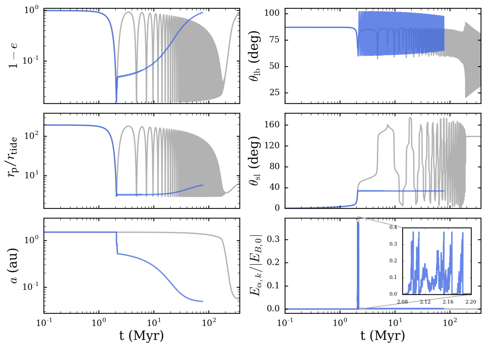
We now discuss our implementation of dynamical tides in giant planet migration driven by the Lidov-Kozai (LK) mechanism. In this scenario, an external stellar or planetary companion induces quasi-periodic oscillations in the eccentricity of the giant planet’s orbit; as the eccentricity attains a large value , tidal dissipation in the planet at pericentre reduces the orbital energy, leading to circularization and decay of the planet’s orbit. As noted in Section 1, previous works on LK migration adopted the (parametrized) weak friction theory of static tides (ST). The grey curves of Fig. 6 give an example of this “standard" LK migration scenario.
The theory of LK migration with static tides involves two important timescales. The first is the timescale for quadrupole LK eccentricity oscillations, , given by
| (40) |
where is the initial semi-major axis of the planet’s orbit, is the mass of the (stellar) companion, and
| (41) |
with and the semi-major axis and eccentricity of the companion’s orbit. The time that the planet spends near the maximum eccentricity, , is of order (Anderson et al. 2016, e.g.)
| (42) |
The second important timescale is that of orbital decay due to static tides given by (Alexander 1973; Hut 1981).
| (43) |
where is the tidal Love number of the planet, is the lag time, , and and are given in equations (30) and (31). (We have assumed that the planet has a pseudosynchronous spin rate.) Tidal dissipation is most efficient near the maximum eccentricity. Since the planet only spends a fraction () of the time near , the effective orbital decay rate during LK migration is
| (44) |
where is the minimum pericentre distance (in the second of the above equalities, we have used ). Successful migration within a few Gyrs requires au, corresponding to a final (circularized) planet semi-major axis au. A planet would need to be more dissipative than Jupiter (larger )55 5 For Jupiter, s, corresponding to at a tidal forcing period of hrs. to become a HJ with a larger .
As we shall see, chaotic tides can change the standard LK migration scenario in several important aspects (see Fig. 6). Although the planet spends only a small fraction of time in the high-eccentricity phase of the LK oscillations, this time covers enough orbits to allow chaotic mode growth. Consider the example depicted in Fig. 6: the critical eccentricity (for au) for chaotic mode growth to operate is (see Fig. 3 and equation 32). So the time the planet spends around is Myr, which is more than orbital periods. The planet’s oscillation mode can grow to a large amplitude within this time frame, stealing orbital energy in the process and allowing the orbit to decay within one or a few LK cycles.
3.1 Description of the Model
We now describe our method for coupling the evolution of the oscillation mode (the f-mode) of a gas giant with the evolution of its orbit driven by an external binary companion (LK oscillations). The planet starts out with eccentricity and zero mode amplitude (). The other planet and stellar properties as well as the initial values of , , , (the mutual inclination of the orbits) and (the longitude of the ascending node of the planet’s orbit) are taken as input parameters. Apart from dynamical tides, we evolve the orbital angular momentum vector and eccentricity vector of the planet, and the spin angular momentum vector, of the host star in the same way as in Anderson et al. 2016 (hereafter ASL16), i.e.
| (45) | ||||
| (46) | ||||
| (47) |
Here the LK terms are contributions (to the octupole order) from the binary companion that give rise to LK oscillations [equations A1-A2 of ASL16; from Liu et al. 2015]; the SL terms arise from the spin-orbit coupling between the host star spin, , and the planet’s orbital angular momentum (equations 60-61 of ASL16); and the short-range force (SRF) terms account for periastron precession of the planet’s orbit due to general relativity (GR) and tidal/rotational distortions of the planet (sections A3 and A4 of ASL16). The stellar spin evolution includes the spin-down torque due to magnetic braking (MS), i.e.
| (48) |
where is taken to be yr to model a solar type star, is the moment of inertia of the star, and is its rotation rate. We assume an initial spin period of 2.3 days. We also evolve the angular momentum and eccentricity vectors of the outer orbit ( and ) according to the octupole LK effect (Liu et al. 2015, equations 19 and 20 of); these changes in the outer orbit are small because . Throughout evolution, we take the planet’s rotation rate to be the pseudosynchronous rotation rate given by equation (29). Equations (45)-(46) include contributions from the dissipation of static tides (ST); these are parameterized by the tidal lag time , and are distinct from the effects of dynamical tides.
In the presence of dynamical tides, we must supplement equations (45)-(47) with the evolution of the mode amplitude. This is based on the iterative map discussed in Section 2.1. Here, we provide a summary of the implementation of this procedure. At a certain time in the orbital evolution, just before the -th pericentre passage, the orbital parameters are and , the planet spin rate is , and the mode amplitude is . To advance to the next orbit, we carry out the following steps:
(i) Calculate from equations (21), (25), and (27) using mode parameters from Table 1 and the current orbital/planet parameters (i.e. , , , etc.) and obtain . In practice, we normalize mode energy by (the initial orbital energy), and thus .
(ii) Calculate the energy transfer in the -th passage using (see equation 17) and obtain the new orbital energy .
(iii) Obtain the new orbital semi-major axis and eccentricity (after the -th pericentre passage) according to
| (49) | ||||
| (50) |
where we have assumed that the orbital angular momentum is conserved during the passage.
(iv) Evolve the (complex) mode amplitude over one orbit to obtain its value just before the -th passage using (see equation 14), where is the orbital period corresponding to and is the mode frequency after the -th passage (assuming a pseudosynchronous rotation rate).


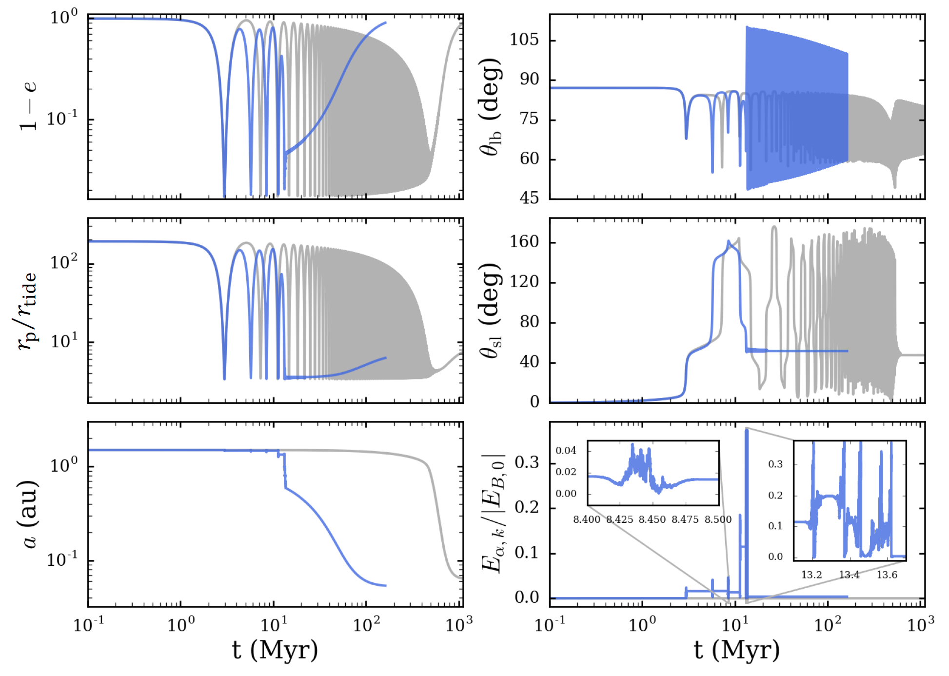
Left unchecked, the mode energy in this model can grow to un-physically large values (as in the bottom panel of Fig. 2). We therefore assume that, when the mode energy reaches a significant fraction of the planet’s binding energy, non-linear effects dissipate nearly all of the mode energy within an orbital period. We parametrize the maximum energy that the mode can reach before non-linear effects become important, , and the residual energy in the mode after an episode of nonlinear mode dissipation and tidal heating, . Thus, when , the mode amplitude is immediately changed to . This method for handling dissipation was used in Wu 2018. The parameter does not change the qualitative features of evolution due to chaotic tides (see Fig. 7), but can alter the details. The quantity is more important because chaotic behaviour is easier to excite when the f-mode already has some energy, as discussed in Section 2.4, but still does not change the overall behaviour of the model (see Fig. 8). Unless stated otherwise, we use and in the results presented in this paper.
Since dynamical tides must be implemented on an orbit by orbit basis, it is not practical to evolve the whole system over many Myrs. Because dynamical tides are effective only during the high-e phase of the LK cycle, when chaotic mode growth occurs, we only need to evolve the modes when the eccentricity is sufficiently high and the pericentre distance is sufficiently small. As discussed in Section 2.5, chaotic tides operate when (see equation 38). In our implementation, we turn on dynamical tides only when . As we see from Fig. 4, this is a conservative choice, allowing us to capture the onset of chaotic behaviour for all reasonable parameters regardless of resonances and the value of “pre-existing" mode energy.
After the orbit has decayed through chaotic tides, the system will eventually satisfy (see the right panel of Fig. 4) while the orbital eccentricity is still large. This typically occurs just after the mode energy is dissipated non-linearly from to . Thus, when the system satisfies
| (51) |
(where we have assumed ) the f-mode will no longer behave chaotically and influence the orbital evolution. Instead, static tides drive the gradual decay and circularization of the planet’s orbit. To save computation time, when equation (51) is satisfied while the orbital eccentricity is large, we take note. If equation (51) is still satisfied in 30,000 orbits, we stop evolving the dynamical tides; if equation (51) is not satisfied after 30,000 orbits, we check again in another 30,000 orbits. The multiple checks are to account for the fact that varies significantly depending on the orbital period and can be less than 1.
3.2 Examples of the Model
LK migration with chaotic tides proceeds in three steps (see the blue curves in Fig. 6). First, the external companion drives the planet’s orbital eccentricity beyond (see equation 32), where chaotic tides set in and begin to take over orbital evolution, freezing due to angular momentum conservation. The blue lines in Figs. 7 and 8 show a zoom-in view. We see that decreases due to the LK effect until settling to an approximately constant value around 2.1 Myr while and start to wander chaotically. In the second stage, chaotic tides dominate orbital evolution and quickly shrink the orbit until it is too bound for such tides to continue operating. In Figs. 7 and 8, it is clear that the planet undergoes multiple episodes of non-linear dissipation (where the mode energy rapidly dissipates to a small residual value of after climbing to maximum energy ) while subject to chaotic tides. The result is a very eccentric WJ. At this new semi-major axis, the planet is decoupled from the influence of the stellar companion, and no longer experiences significant eccentricity oscillations. Finally, weak tidal friction circularizes and shrinks the orbit to form a HJ on a Gyr timescale (depending on the dissipation rate of static tides in the planet).
In some cases, a system will undergo multiple high-eccentricity phases before chaotic tides reach the threshold and the f-mode dissipates energy. An example is shown in the blue lines of Fig. 9, where the system has the same parameters and initial conditions as in Fig. 6 but with a slightly larger companion semi-major axis ( au). We see that the planet’s eccentricity undergoes five LK oscillations before the f-mode energy climbs to . Before an episode of tidal dissipation, any energy transferred from the orbit to the mode can easily pass back to the orbit. For example, in the third high-eccentricity phase of Fig. 9 (shown in an inset of the bottom right panel) the f-mode loses a small amount of energy and the semi-major axis increases slightly. Once the mode energy reaches and is dissipated, the orbit shrinks irreversibly and continues to rapidly decay until the orbit is too bound for chaotic tides to operate.
We can gain some insight into when a system requires multiple high-eccentricity phases to reach by studying the rate of chaotic orbital decay predicted by the iterative map from Section 2.1. While (for ), the mode amplitude grows in an approximately diffusive manner [Fig. 5 of Vick & Lai 2018; see also Mardling 1995a; Ivanov & Papaloizou 2004; Wu 2018], with the averaged mode energy
| (52) |
For a sufficiently eccentric orbit, is roughly constant over many pericentre passages. We can define a timescale for orbital decay from the energy transfer and dissipation,
| (53) |
If we use the largest value of attained by the system in Fig. 9, we find that Myr and the timescale for the system to remain at high eccentricity is Myr (see equation 42). Because , the system must undergo multiple LK cycles for the mode energy to climb to . In contrast, the system in Fig. 6 reaches , for which Myr and Myr. For this system, where the timescale for chaotic tides to alter the orbit is very short, the planet’s orbit decays within one high-eccentricity phase.
4 Key Features of Chaotic Tidal Migration: Analytical Understanding
LK migration with chaotic tides has a few characteristic features. First, it can prevent some gas giants from undergoing tidal disruption. Second, it naturally produces very eccentric WJs. Lastly, this population of WJs circularizes relatively quickly, due to weak tidal friction because the planets are “detached" from the companions’ perturbations. In the following, we discuss the necessary conditions for LK chaotic tidal migration, hallmarks of this process, and predictions for the stellar obliquities of HJs formed via this mechanism.
4.1 Condition for Chaotic Tidal Migration
As discussed in Section 2.3, a planet must have to initiate chaotic tides, where as a function of (the initial semi-major axis of the planet) is implicitly given by equation (32). To reach such a high eccentricity, a system must have sufficiently large initial mutual inclination, . In the idealized case of quadrupole LK oscillations, the maximum eccentricity is Accordingly, can be achieved only for . Including octupole terms complicates the relationship between the initial mutual inclination and the maximum attainable eccentricity and broadens the inclination window for extreme eccentricity excitation. A realistic treatment of the LK effect must also account for the short-range forces (SRFs) that cause the planet’s pericentre to precess. These limit the maximum attainable eccentricity in LK cycles to a value , where is the maximum eccentricity achieved when in the quadrupole limit. In the presence of the octupole potential, the eccentricity still cannot exceed , but this eccentricity can be realized for a wider range of initial inclinations (Liu et al. 2015). The relevant SRF’s for this problem are GR and the effect of static tides raised on the planet. When , the limiting eccentricity is given by
| (54) |
where and measure the strengths of precession due to GR and the planet’s tidal bulge relative to the quadrupole LK effect, respectively:
| (55) | ||||
| (56) |
For our “standard" system (shown in Fig. 6) with au, au, and , we find and , so the planet can reach large enough eccentricities to experience chaotic tides, provided the initial mutual inclination angle, , is sufficiently large.
In general, the necessary condition for chaotic tidal migration is
| (57) |
or equivalently , where and are given by equation (32) (or more approximately by equation 34). Because , given by equation (54), depends on , the condition on translates to an upper limit on for chaotic migration to occur:
| (58) |
The upper limit in equation (58) is shown as a blue line in Fig. 10.
We can also derive the maximum that allows for standard LK migration with static tides within a stellar lifetime. Using equation (44) and requiring that the planet migrate within (i.e. ), we find
| (59) |
[ is called in Muñoz et al. 2016]. Substituting for in equation (58) yields an approximate maximum for standard LK migration (without chaotic tides). The result is shown as the dashed line in Fig. 10. For a , gas giant, the conditions for chaotic tidal migration are typically more generous than for standard LK migration. This suggests that LK migration with chaotic tides yields more HJs than LK migration with static tides.

4.2 Evading Tidal Disruption
The planet can be tidally disrupted if its pericentre distance, , is less than the tidal disruption limit from equation (24),
| (60) |
Therefore, when , the companion can induce tidal disruption of the planet if is sufficiently large. Substituting for in equation (58) yields the maximum for tidal disruption to be possible. This is shown as the red line in Fig. 10.
In the standard LK migration scenario (with static tides), a large fraction of migrated giant planets are tidally disrupted because can be quite close to ; moreover, Saturn-mass planets can rarely migrate successfully via LK oscillations and static tides because (Muñoz et al. 2016, ASL16,). In contrast, with chaotic tides, there is always a region of parameter space where chaotic tidal migration is possible without disruption (; see Fig. 3) for any reasonable values of and for giant planets.
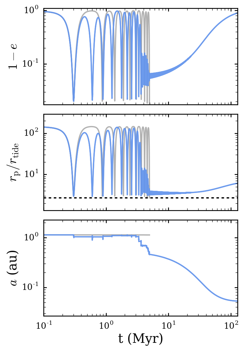
In some cases, chaotic tides can shepherd to safety the planets that are otherwise destined for tidal disruption by acting to rapidly decrease and increase . This possibility was suggested in Wu 2018. Figure 11 shows one such example. Before the planet is pushed to extreme eccentricity and tidal disruption by the octupole potential, it is frozen into a high-eccentricity orbit with a small semi-major axis and becomes decoupled from the companion. Without further interference from the LK effect, the eccentric WJ circularizes in orbit over a Gyr timescale to eventually become a HJ.
We can understand the condition for chaotic tides to save a planet from disruption using a simple time-scale argument. Tidal disruption occurs when . At high eccentricity, the timescale for a planet to remain below a given is (see equation 42), while the timescale for chaotic tides to decay the orbit is , given by equation (53). The planet reaches a minimum when these timescales are roughly equal. For planets that are “just saved" from disruption, this minimum is nearly . A system that can be saved from disruption must satisfy , i.e.
| (61) |
where is evaluated at (see equation 21). Recall that depends on . When , and the pseudosynchronous spin rate, , have negligible dependence on . We can then evaluate by using equation (25) with the approximate from equation (27) and taking for the mode frequency in the inertial frame. At , .
4.3 Eccentric Warm Jupiter Formation

A giant planet that undergoes chaotic orbital decay becomes an eccentric WJ after reaching a semi-major axis where both chaotic tides and the LK effect have little influence on the continued evolution of the planet’s orbit. For example, in Figs. 6 - 8, all of the integrations produce a planet with a semi-major axis between and au and an eccentricity between 0.93 and 0.97. We can understand why this occurs by re-examining the criterion for chaotic tides to stop affecting orbital evolution (see equation 51). Typically, chaotic tides end just after a dissipation episode, where . Setting with and , we find
| (63) |
where and are evaluated at , the pericentre distance of the planet when chaotic tides stop operating. The value of varies erratically for small changes of initial conditions, but must fall between () and (very roughly ) for a system with au. Equation (63) gives the relationship between and for WJs formed by chaotic tides. Parametrizing the residual mode energy by , and using equation (21), we can write in terms of the planet properties and :
| (64) |
Equation (64) is plotted in Fig. 12 for two different planet models. For values of between and , equation (64) yields semi-major axes in the range of au (for and ). We can also find the eccentricity of the WJs via
| (65) |
For between and , is between 0.027 and 0.060 (again for and ).
Figures 6, 9, and 11 show that after the WJ forms through chaotic tides, the eccentricity freezes at a high value and the planet’s orbit decouples from the companion. In general, LK eccentricity oscillations freeze when where is the rate of precession due to SRFs. This is equivalent to or . We find that tidal effects play a more important role than GR in the “freezing" of eccentricity oscillations of WJs.
4.4 Fast Long-Term Orbital Decay and Hot Jupiter Formation
When the planet’s orbit is no longer strongly influenced by chaotic f-mode evolution and the LK effect, the orbit decays and eventually circularizes due to tidal friction from static tides raised on the planet. The final result is a HJ. This is the same mechanism that has been used to explain HJ formation in previous studies of migration via the LK effect (Petrovich 2015a, ASL16;). Here, the process occurs more quickly because the orbit is frozen into a small pericentre value rather than oscillating between high and low eccentricities. Figures 6 and 9 compare the long-term orbital evolution predicted by our model (in blue) with the standard calculation that does not include chaotic tides (in grey). In both cases, the orbit circularizes much more quickly when chaotic tides are included.
4.5 Spin-Orbit Misalignment and Final Planet-Binary Inclination
Recent studies (Storch et al. 2014; Storch et al. 2017, ASL16) have shown that a giant planet undergoing LK migration can induce complex dynamics in the spin axis of the oblate host star before the spin-orbit misalignment angle (stellar obliquity), , becomes frozen. This freezing occurs when the precession rate, , of the stellar spin vector () around (the unit orbital angular momentum vector of the planet) becomes much faster than the precession rate () of around the binary angular momentum axis . The ratio of precession rates is
| (66) |
where
| (67) |
and
| (68) |
with as the stellar moment of inertia constant, as the stellar rotational distortion coefficient, and as the stellar spin rate (see ASL16). We take = 0.1 and . We call the adiabaticity parameter. The spin-orbit angle freezes when .
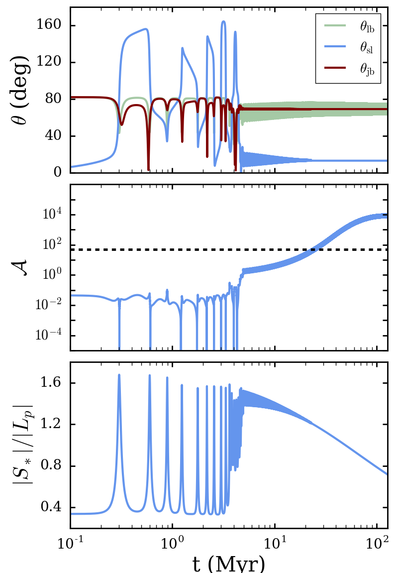
Figure 13 shows an example of the evolution of the spin-orbit misalignment angle during chaotic tidal migration. The stellar spin rate evolves according to the Skumanich law given in equation (48). When chaotic tides stop operating, around 4.5 Myr, , and still oscillates with an amplitude of . Because depends on the stellar spin rate and , the condition for the adiabatic “spin-orbit freeze" () is generally different from the condition for “LK oscillations freeze" [; see section 4.3]. Many of the planets that migrate via LK chaotic tides will not have a fixed when they become eccentric WJs.
The mutual inclination between the orbits of the planet and the stellar companion is also of interest. We see from Fig. 13 that can oscillate even at the end of the evolution (when the planet has become a HJ). This variation of arises from the coupling between and (with non-negligible compared to ). We define
| (69) |
We find that the angle between and , , is constant when the planet’s orbit is decoupled from the influence of the stellar companion. To understand this, consider the time evolution of the planet’s orbital angular momentum axis and the stellar spin axis . Both are rapidly precessing around . An external torque acting on (from magnetic braking) or (from the binary companion) also acts on . But after averaging over the fast timescale , the net effect is that precesses around . As a result, is constant and oscillates around with amplitude , where
| (70) |
The top panel of Fig. 13 illustrates this behaviour. As the star gradually spins down due to magnetic braking, asymptotes to .
5 Population Synthesis
In this section we carry out a population synthesis study of giant planets undergoing LK migration with chaotic tides. Our goal is to determine the production efficiencies of eccentric WJs and HJs, as well as their general properties as predicted by this scenario.
| 1 , 1 | 1.6 , 1 | 1.6 , 0.3 | ||||||
|---|---|---|---|---|---|---|---|---|
| Rate | Prediction | Rate | Prediction | Rate | Prediction | |||
| 14.0 % | 13.7 % | 15.4 % | 14.2 % | 16.7 % | 15.2% | |||
| 10.1% | 11.9% | 11.5 % | 11.9 % | 13.2 % | 13.1 % | |||
| 3.9% | 1.8 % | 3.9% | 2.3 % | 3.6 % | 2.1 % | |||
| 3.9% | — | 3.8% | — | 2.2 % | — | |||

5.1 Setup and Method
All of our population synthesis calculations use the same stellar and companion masses . The initial rotational period of the host star is days, and the star spins down according to the Skumanich law (equation 48). The planet model is a polytrope. We consider two planet radii, and , and two planet masses and .
While some of our earlier examples have assumed that (so that the octupole terms vanish), in the population synthesis we consider a broad range of and incorporate the octupole LK effect. The importance of the octupole effect (relative to the quadrupole effect) is encoded in the dimensionless parameter
| (71) |
We have explored a variety of initial conditions, uniformly spanning , (au) (uniformly sampled in ), , and (where is the initial longitude of the ascending node of the planet’s orbit). Our choice of initial mutual inclinations, , is limited to the range where the quadrupole LK effect can operate, i.e. . Systems that do not obey the stability criterion (Mardling & Aarseth 2001),
| (72) |
are discarded. Note that the range of initial conditions is identical to that of ASL16 for straightforward comparison between the HJ formation fraction from LK migration with and without chaotic tides.
The details of how the evolution of the planetary f-mode is calculated in combination with the LK effect are discussed in Section 3.1. In all calculations, we use and to parametrize the maximum f-mode energy and the residual energy after an episode of non-linear tidal dissipation. The planet is assumed to be rotating at the pseudo-synchronous rate (equation 29). The effect of dynamical tides on the planet’s spin is not accounted for in this investigation, but could be incorporated into future studies that follow the evolution of multiple oscillatory modes in the planet.
Our study is structured to efficiently determine the likelihood of three possible outcomes: “No Chaotic Tidal Migration", “Tidal Disruption", and ‘Chaotic Tidal Migration". Each calculation is stopped when the integration time reaches 1 Gyr or when one of the following conditions is met:
(i) If (equation 38) has not reached 1 after min, the calculation is terminated and the system is labelled as “No Chaotic Tidal Migration". Note that a small percentage of such systems may migrate within 1 Gyr via standard LK migration without the assistance of chaotic tides. These are not identified as a separate outcome from planets that will not migrate at all.
(ii) If the system has evolved for more than planetary orbits in the chaotic phase (i.e. where the orbital evolution is coupled with the f-mode evolution, as discussed in Section 3.1) without reaching , the integration is stopped and the system is classified as “No Chaotic Tidal Migration".
(iii) If, at any time, the pericentre distance is within the tidal disruption radius, i.e. , the outcome is classified as “Tidal Disruption", and the integration is stopped.
(iv) If the planet has experienced chaotic orbital evolution and its orbit has circularized to within 1 Gyr, the integration is stopped and the system is classified as having undergone “Chaotic Tidal Migration".
For each system, we begin by integrating the full equations of motion and incorporating the evolution of the planet f-mode (as described in Section 3.1). However, at different points in the giant planet’s evolution, it is possible to “turn off" various effects without losing accuracy. As discussed in Section 3.1, the effect of dynamical tides is only accounted for when it can significantly affect orbital evolution. Additionally, when the semi-major axis is small, LK oscillations are suppressed. As the planet’s orbit shrinks and circularizes on a long time-scale due to static tides [see equation (43) with s], the eccentricity of the planet’s orbit precesses on a much shorter time-scale than that of tidal decay. Following this precession is computationally expensive and does not affect the final properties of the migrating planet. When the LK oscillations are “frozen" [] and the spin-orbit angle is safely adiabatic (), we continue the integration without LK and SRF terms.
5.2 Migration and WJ/HJ Formation Fractions
The results of our population synthesis are summarized in Table 2. For each combination of planetary mass and radius, we ran calculations to determine the fraction of systems that undergo chaotic tidal migration (). These migrated planets are either tidally disrupted (fraction ) or survive as eccentric WJs (fraction ) that undergo further orbital decay and circularization due to static tides, eventually becoming HJs. The fraction of systems that evolve into HJs within 1 Gyr is denoted by . Note that our population synthesis did not sample initial mutual inclinations with , as such planets do not experience large excursions in eccentricity. The migration, disruption, WJ, and HJ fractions are calculated assuming a uniform distribution in , e.g. with the number of systems that displayed chaotic tidal migration and the total number of runs. For , planets, the HJ formation percentage from our population synthesis is larger than the value obtained for standard LK migration by a factor of (3.9 % vs 2.4 %); see(Muñoz et al. 2016, ASL16;).
5.3 Parameter Space for WJ Formation
We can learn about the parameter space that leads to eccentric WJ formation by examining how the outcome of orbital evolution depends on the initial conditions and the planet properties (see Fig. 14; see also Fig. 18 from ASL16 for comparison with the standard LK migration results). It is clear that smaller values of do not yield migration. This is unsurprising as the eccentricities required for chaotic tides are very large, which necessitates large initial mutual inclinations. Another pronounced feature is that the systems that produce eccentric WJs are clustered in . The reason for this is discussed in Section 4 (see Fig. 10). In essence, only a narrow window in can produce systems that will reach large enough eccentricities to undergo chaotic tides (see equation 58), but not so large that the planets are tidally disrupted (see equation 62). Figure 15 demonstrates that the systems that produce surviving WJs indeed satisfy equations (58) and (62). The range of that can produce eccentric WJs is capped by the limit on (see equation 71). Lastly, Fig. 14 shows that changing the properties of the gas giant has little effect on the parameter space that produces eccentric WJs. Unlike standard LK migration with static tides, where systems with produce hot Saturns at a rate of (assuming s) after evolving for 5 Gyr (Muñoz et al. 2016, see ASL16,), chaotic tides allow low-mass planets to survive high-eccentricity migration without suffering tidal disruption, and produce hot Saturns at a rate of about after only 1 Gyr.

5.4 Properties of WJs Formed by Chaotic Tidal Evolution


We now examine the orbital properties of planets produced by chaotic tides. The scatter plots in Fig. 16 show an overview of the WJ eccentricities and semi-major axes ( and ) for the planet model after the planetary f-mode has settled into a quiescent state (but before weak tidal friction circularizes the orbit over a long time-scale). Most planets have between and au and between 0.91 and 0.97. Systems that have undergone multiple LK cycles tend to have larger and . This is expected because larger values of and correspond to systems that do not reach a small enough value of for chaotic tides to significantly alter the orbit within the time-frame of a single high-eccentricity phase. In general, and increase with [see equations (64) and (65) and Fig. 12].
In the top left panel of Fig. 16, the values of seem to fall on a set of - curves. This feature arises from our treatment of non-linear dissipation, where the f-mode rapidly dissipates energy after reaching . Each curve corresponds to some number of non-linear dissipation episodes, after which the orbital energy becomes . The systems with the most distant stellar companions can produce WJs with relatively large semi-major axes (1 au) after chaotic tidal evolution. This occurs because the minimum required for chaotic tides to compete with the LK effect is larger for systems with larger . In Fig. 16, we can also see that most systems that exhibit chaotic behaviour have initial mutual inclinations around , as expected. Lastly, as seen earlier in Fig. 14, large values of do not produce surviving WJs.
Figure 17 shows the histogram of the parameters of WJs produced by chaotic tidal migration. The distributions of planet properties are generally more sharply peaked for denser planets. The ranges of and are in agreement with equations (64) and (65), which predict that scales linearly with while has no dependence on the planet radius and a weak dependence on the planet mass (for a given minimum achieved during the orbital evolution). Combining equations (64) and (65), we can see that the distribution of should scale directly with . This would imply that the peak at au in the distribution for the planet model should appear near au and au in the and models, respectively, as is the case in Fig. 17. The timescale for chaotic evolution to shrink the orbit, , peaks near 10 Myr for all planet models.
The range of is narrow for all three planet models. The lower edge of this distribution is determined by the tidal disruption radius. A planet cannot survive if . The upper value of is roughly set by the pericentre distance where the planet with the largest semi-major axis (in our simulation, au) crosses the chaos boundary, generally near . Figure 18 shows the relationship between , and for planets that have undergone chaotic evolution. The solid lines show equation (65) for each planet model. Recall that equation (65) yields the eccentricity where for a given . Therefore, the restrictions on determine the range in the distributions of and . This simple calculation explains the properties of planets that survive chaotic tidal evolution very well. The spread in the results from the population synthesis arises from the fuzziness in the chaotic tides boundary, i.e. variations in . These variations are larger for smaller (see Fig. 4). On average, systems with smaller and larger have smaller . Accordingly, the spread in the results is largest for the model and smallest for the model.
5.5 Hot Jupiter Properties
The eccentric WJs formed by chaotic tidal migration continue to experience orbital decay and circularization due to static tides. As long as the static tide is sufficiently dissipative, the planet will circularize to
| (73) |
For our population synthesis, most WJs circularize within 1 Gyr (assuming s) to become HJs (see Table 2). Those that do not are almost exclusively from the low-density planet model with the largest . The HJ period distributions for our population synthesis calculations are shown in Fig. 19. The peak lies between 3.5 and 4 days for our standard model with ; this shifts to smaller periods for denser planets (with , ). As discussed in Section 5.4, the range of is set by the pericentre distance requirements for tidal disruption and for chaotic tidal behaviour. Both of these conditions vary directly with , so the peak of the HJ period distribution scales as .
The final spin-orbit misalignments () are also shown in Fig. 19. For all three planet models, the distribution in is bimodal, peaking near and . These distributions are qualitatively similar to those obtained in ASL16 for standard LK migration with static tides. In general, the percentage of retrograde configurations () is larger for chaotic tidal migration than for standard LK migration. This may be due to the fact that, because chaotic tides dramatically speed up orbital decay, the star is rotating more rapidly when becomes “frozen," and the feedback torque from the star on the orbit is larger.
We have also provided the final values of , the angle between and . In all of our calculations, the ratio is still of order unity near (the time when the planet’s orbit has circularized to ), so the mutual inclination of the inner and outer orbits, , is not fixed at . As the star continues to spin down, will approach , as discussed in Section 4.5. The distributions of have two strong peaks around and .
Lastly, Fig. 19 shows the distribution of “arrival times" for HJs, , when . For the planet model, all orbits circularize to within 1 Gyr. For the model, only 65% of the WJs circularize within a Gyr timeframe, yet 97% can become HJs within 10 Gyr. In general, planets with larger finish chaotic evolution at larger and take longer to circularize via static tides. Most planets that undergo chaotic tidal evolution can be expected to become HJs within the lifetimes of their host stars. As a result, the population of eccentric WJs formed by chaotic tides is transient (assuming s).


6 Analytical Calculation of WJ Formation Fraction
Muñoz et al. 2016 developed an analytical method to calculate the HJ formation fraction in the standard LK migration (with static tides) scenario. In this section, we adapt this method to calculate the fractions of systems that experience chaotic tidal migration or tidal disruption. A system will become chaotic or suffer disruption when the planet’s pericentre distance is smaller than a critical value — for chaotic behaviour, from equation (34), for disruption, from equation (60). We define as the minimum initial mutual inclination necessary for a system to reach , or equivalently (see equation 32). Assuming uniform distribution in , the fraction of systems (for a given , , ) that experience chaotic tidal behaviour is then
| (74) |
where when . We refer to Muñoz et al. 2016 for the calculation of given . By performing a Monte Carlo integration over (au), (au) (uniformly sampled in ), and , we can predict the fraction of systems in our population synthesis where the planet undergoes chaotic tidal migration () and fraction of systems where the planet is tidally disrupted (). The fraction of systems that become chaotic but are not disrupted is given by
| (75) |
As discussed in Section 4.2, chaotic tides can compete with the LK effect and prevent planet tidal disruption. Our analytic calculations therefore provide an upper limit to the tidal disruption fraction () and a lower bound on the fraction of WJs formed () in this scenario. Table 2 shows that our analytical results are in good agreement with the populaion synthesis results. Our analytical is slightly smaller than the value obtained from population synthesis, likely because the boundary for chaotic tides is fuzzy and we have chosen a conservatively low value for .
In addition to calculating and , we can estimate the total migration fraction where the planet either migrates via chaotic tides or migrates within 1 Gyr due to weak tidal friction (the standard LK migration scenario). For a given , and , this is
| (76) |
where is the maximum value of for which a system can reach , given in equation (59). We can integrate over orbital parameters , , and (as before) to find . Because is generally less than , the percentage of systems that are not chaotic but become HJs due to weak tidal friction is much less than .
In our population synthesis calculations (Section 5) we have only considered planets with and and radius or . With analytic calculations, we can easily predict the fractions of systems that survive chaotic tides or suffer disruption as a function of and . The results are shown in Fig. 20. The fraction of systems that undergo chaotic tidal migration is nearly independent of , (%). The WJ formation fraction from LK chaotic tides is also insensitive to and because and have roughly the same scaling with and . This result differs from the standard picture of LK migration, where Saturn-mass planets that migrate are destined for tidal disruption (see ASL16).

7 Summary and Discussion
7.1 Summary of Key Results
In this paper, we have systematically studied the role of dynamical tides in high-eccentricity gas giant migration via the LK effect. Our investigation has revealed (i) the conditions under which dynamical tides in the planet have a significant effect on migration, (ii) the characteristics of the planet population that results from LK migration with dynamical tides, and (iii) the expected HJ fraction from this formation path. The overall summary of the paper is already given in the abstract. Here we provide a guide to the key results of each section.
In Section 2, we explored the orbital parameters necessary for a gas giant to undergo chaotic tidal migration. When a planet’s orbit is very eccentric and its pericentre distance is sufficiently small, the tidal force from the host star can excite planetary oscillations at pericentre in such a way that these oscillations chaotically climb in amplitude over repeated close passages (an example is shown in the bottom panel of Fig. 2). We found that, for the polytrope planetary model, the fundamental mode (f-mode) is more strongly excited than inertial modes, and is the most likely to experience chaotic growth over multiple orbits. The condition for these “chaotic tides” to operate is given by equation (32) and plotted in Fig. 3. In general, chaotic tides can occur in planets on highly eccentric orbits with small pericentre distances. We also explored (in Sections 2.4 and 2.5) how the conditions for chaotic tides become more generous when the f-mode already has some non-zero energy.
In Section 3, we developed a model to couple the LK migration with orbital changes due to dynamical tides. The model is fully described in Section 3.1, and can be readily adapted to other high-eccentricity migration mechanisms. Although the model is largely ab initio, there are two free parameters that characterize the (uncertain) nonlinear mode dissipation: (the maximum energy the mode can reach before nonlinear dissipation sets in) and (the residual energy in the mode after an episode of nonlinear dissipation). We found that these parameters (with reasonable values) do not change the general features of evolution due to chaotic tides, but can alter the details (see Figs. 7-8).
In Sections 3.2 and 4, we presented example calculations of the LK chaotic tidal migration, and explained some key features of this migration mechanism:
- •
Chaotic tidal migration leads to rapid formation of WJs (see Fig. 6 for an example) on timescales a few to 100 Myrs (see Fig. 17). These WJs have eccentricities in the range and semi-major axes between 0.1 and 2 au (with lower values more likely), depending on the giant planet mass and radius (see Fig. 16).
- •
These eccentric WJs efficiently circularize to HJs via dissipation of static tides. This process is faster than standard LK migration because a planet that experiences chaotic tides quickly becomes decoupled from the influence of the perturber and the eccentricity oscillations are frozen (see Figs. 6, 9 and 11).
- •
In Section 5, we conducted a population synthesis study to determine the formation fractions and properties of eccentric WJs and HJs for a few combinations of planet mass and radius. Our study sampled the same range of initial orbital parameters as in Anderson et al. (2016) for the standard LK migration scenario. The calculated fractions for chaotic tidal migration (), tidal disruption (), WJ formation (; note that ) and HJ formation within 1 Gyr (), are provided in Table 2. For an planet, LK chaotic tidal migration produces more HJs than standard LK migration ( increases from to ; see Table 3 in ASL16). More importantly, chaotic tides can produce hot giant planets with a broad range of masses and radii. This is in stark contrast with the standard LK migration, which produces very few hot Saturns because of the severe tidal disruption experienced by such low-mass giants (ASL16; Munoz et al. 2016).
The orbital properties of planets from our population synthesis that survived chaotic tidal migration are shown in Figs. 17 and 19. The WJs that are produced directly by chaotic tidal dissipation have pericentre distributions that peak near . These pericentre values are smaller than those of observed high-eccentricity WJs such as HD80606 b (Hébrard et al. 2010). This is expected as the eccentric WJs formed by chaotic tides are “transient” and should move quickly through the high-eccentricity phase. The HJs that form via LK chaotic tidal migration exhibit a pile-up around a 3 day orbital period, depending on the planet’s mass-radius relation and the assumed tidal disruption criterion. This is a feature of all tidal migration mechanisms. However, our predicted HJ period distribution for LK chaotic tidal migration differs from that for the standard LK migration, particularly for low-mass giant planets (compare Fig. 19 with the middle row of Fig. 23 from ASL16). Chaotic tidal migration can produce Saturn-mass planets at periods longer than 5 days and generates a wider period distribution for such planets. Finally, we found that chaotic tidal migration yields similar spin-orbit misalignments as the standard LK migration (compare Fig. 19 with Fig. 24 of ASL16). For all three planet models we considered, the distribution of final spin-orbit misalignments is bimodal with peaks at and .
In Section 6, we used an analytical method, developed in Muñoz et al. 2016, to understand how the HJ formation rate varies with planet mass and radius. We calculated a lower-bound on the eccentric WJ formation rate (not accounting for planets that are spared from tidal disruption by chaotic tides). The predicted (analytical) rates are in agreement with the results from the population synthesis study (see Section 5) and are shown in Fig. 20. We confirmed that the WJ formation rate from LK chaotic tidal migration is constant over a reasonable range of giant planet masses and radii, as suggested by, e.g., Fig. 14 and Table 2.
7.2 Discussion
The results presented in this paper show that chaotic tides endow the LK migration scenario with a number of “favorable” features (Wu 2018, see also). These not only reduce the theoretical uncertainties regarding tidal dissipation that are inherent in the theory, but also may help reconcile some of the discrepancies between observations and predictions of LK migration. Chaotic tides drastically reduce the amount of time that a gas giant spends at high eccentricity. This could explain the lack of observations of super-eccentric gas giants (Dawson et al. 2015). In addition, chaotic tides quickly decouple a gas giant experiencing LK oscillations from the stellar perturber. This allows planets at larger pericentre distances to migrate within the lifetime of their host stars. In this way, chaotic tidal migration naturally produces a period distribution with a longer tail. Indeed, HJs beyond the 3-day pile-up are observed but difficult to explain with standard high-e migration scenarios.
Although chaotic tides increase the HJ yield from LK migration in stellar binaries, particularly for low-mass planets, we should not expect this particular formation channel to account for all HJs. The occurrence rate of HJs produced by this channel can be computed from
| (77) |
where is the fraction of stars with a binary companion and is the fraction of solar-type stars with a giant planet at a few au. Assuming (Raghavan et al. 2010; Ngo et al. 2015), (as in ASL16), and from our population synthesis calculation, we obtain an estimate of , which is nearly an order of magnitude smaller than the observed occurrence rate of (Marcy et al. 2005; Wright et al. 2012; Fressin et al. 2013). Thus, LK chaotic tidal migration in stellar binaries can roughly account for of the observed HJ population.
However, we expect that many of the “nice” features of chaotic tides may also apply to other flavours of high- migration scenarios, such as LK migration induced by planetary companions and secular chaos in multi-planet systems. The eccentricity and pericentre ranges of planets that are susceptible to chaotic tides are set by the boundary for chaotic f-mode behaviour (see Section 2), and do not depend on a specific high- migration scenario. Chaotic tides can save a planet from tidal disruption when the time-scale for energy transfer to the planet’s oscillation mode is shorter than the time-scale for driving and maintaining the planet’s high-eccentricity (see Section 4.2) – this condition can be satisfied by all secular eccentricity excitation mechanisms. Indeed, the recent work by Teyssandier et al. 2018 showed that chaotic tides significantly increase the HJ formation fraction in the secular-chaos high- migration scenario. Overall, chaotic tides boost the importance of high- migration for the formation of HJs.
The story of chaotic tidal migration hinges upon the planet’s ability to survive rapid tidal heating. There is reason to expect that the planet interior could survive this process (Wu 2018) if most of the dissipated energy goes into the outer layers of the planet, which can quickly radiate heat. However, if the tidal energy is deposited at a larger depth, the planet’s envelope may expand. Such changes in the structure of the planet would affect the f-mode frequency and could have a larger influence on the evolution of the planet’s orbit. A sudden expansion of the planet’s radius may also put the planet in danger of tidal disruption. Many of the planets that survive chaotic tidal migration come close to the tidal disruption radius. Expansion of the planet could easily lead to stripping of the outer layers and initiate mass transfer or mass loss. The effect of mode energy dissipation on the planetary structure is a very important problem for future study.
Acknowledgements
This work is supported in part by the NSF grant AST1715246 and NASA grant NNX14AP31G. MV is supported by a NASA Earth and Space Sciences Fellowship in Astrophysic. KRA is supported by a NASA Earth and Space Sciences Fellowship in Planetary Science.
References
- Albrecht et al. (2012) Albrecht S., et al., 2012, ApJ, 757, 18
- Alexander (1973) Alexander M. E., 1973, Ap&SS, 23, 459
- Anderson et al. (2016) Anderson K. R., Storch N. I., Lai D., 2016, MNRAS, 456, 3671
- Batygin et al. (2016) Batygin K., Bodenheimer P. H., Laughlin G. P., 2016, ApJ, 829, 114
- Beaugé & Nesvorný (2012) Beaugé C., Nesvorný D., 2012, ApJ, 751, 119
- Boley et al. (2016) Boley A. C., Granados Contreras A. P., Gladman B., 2016, ApJ, 817, L17
- Bryan et al. (2016) Bryan M. L., et al., 2016, ApJ, 821, 89
- Chatterjee et al. (2008) Chatterjee S., Ford E. B., Matsumura S., Rasio F. A., 2008, ApJ, 686, 580
- Correia et al. (2012) Correia A. C. M., Boué G., Laskar J., 2012, ApJ, 744, L23
- Dawson & Johnson (2018) Dawson R. I., Johnson J. A., 2018, ARA&A, 56, 175
- Dawson et al. (2015) Dawson R. I., Murray-Clay R. A., Johnson J. A., 2015, ApJ, 798, 66
- Fabrycky & Tremaine (2007) Fabrycky D., Tremaine S., 2007, ApJ, 669, 1298
- Fressin et al. (2013) Fressin F., et al., 2013, ApJ, 766, 81
- Fuller (2014) Fuller J., 2014, Icarus, 242, 283
- Fuller & Lai (2012) Fuller J., Lai D., 2012, MNRAS, 420, 3126
- Fuller et al. (2014) Fuller J., Lai D., Storch N. I., 2014, Icarus, 231, 34
- Guillochon et al. (2011) Guillochon J., Ramirez-Ruiz E., Lin D., 2011, ApJ, 732, 74
- Guillot (2005) Guillot T., 2005, Annual Review of Earth and Planetary Sciences, 33, 493
- Hamers & Portegies Zwart (2016) Hamers A. S., Portegies Zwart S. F., 2016, MNRAS, 459, 2827
- Hébrard et al. (2008) Hébrard G., et al., 2008, A&A, 488, 763
- Hébrard et al. (2010) Hébrard G., et al., 2010, A&A, 516, A95
- Huang et al. (2016) Huang C., Wu Y., Triaud A. H. M. J., 2016, ApJ, 825, 98
- Hut (1981) Hut P., 1981, A&A, 99, 126
- Ivanov & Papaloizou (2004) Ivanov P. B., Papaloizou J. C. B., 2004, MNRAS, 347, 437
- Jurić & Tremaine (2008) Jurić M., Tremaine S., 2008, ApJ, 686, 603
- Kley & Nelson (2012) Kley W., Nelson R. P., 2012, ARA&A, 50, 211
- Knutson et al. (2014) Knutson H. A., et al., 2014, ApJ, 785, 126
- Kochanek (1992) Kochanek C. S., 1992, ApJ, 385, 604
- Kozai (1962) Kozai Y., 1962, AJ, 67, 591
- Kumar & Goodman (1996) Kumar P., Goodman J., 1996, ApJ, 466, 946
- Lai (1996) Lai D., 1996, ApJ, 466, L35
- Lai (1997) Lai D., 1997, ApJ, 490, 847
- Lai & Wu (2006) Lai D., Wu Y., 2006, Phys. Rev. D, 74, 024007
- Lidov (1962) Lidov M. L., 1962, Planet. Space Sci., 9, 719
- Lin et al. (1996) Lin D. N. C., Bodenheimer P., Richardson D. C., 1996, Nature, 380, 606
- Lithwick & Wu (2014) Lithwick Y., Wu Y., 2014, Proceedings of the National Academy of Science, 111, 12610
- Liu et al. (2015) Liu B., Muñoz D. J., Lai D., 2015, MNRAS, 447, 747
- Marcy et al. (2005) Marcy G., Butler R. P., Fischer D., Vogt S., Wright J. T., Tinney C. G., Jones H. R. A., 2005, Progress of Theoretical Physics Supplement, 158, 24
- Mardling (1995a) Mardling R. A., 1995a, ApJ, 450, 722
- Mardling (1995b) Mardling R. A., 1995b, ApJ, 450, 732
- Mardling & Aarseth (2001) Mardling R. A., Aarseth S. J., 2001, MNRAS, 321, 398
- Muñoz et al. (2016) Muñoz D. J., Lai D., Liu B., 2016, MNRAS, 460, 1086
- Nagasawa et al. (2008) Nagasawa M., Ida S., Bessho T., 2008, ApJ, 678, 498
- Naoz (2016) Naoz S., 2016, ARA&A, 54, 441
- Naoz et al. (2012) Naoz S., Farr W. M., Rasio F. A., 2012, ApJ, 754, L36
- Narita et al. (2009) Narita N., Sato B., Hirano T., Tamura M., 2009, PASJ, 61, L35
- Ngo et al. (2015) Ngo H., et al., 2015, ApJ, 800, 138
- Ogilvie (2014) Ogilvie G. I., 2014, ARA&A, 52, 171
- Petrovich (2015a) Petrovich C., 2015a, ApJ, 799, 27
- Petrovich (2015b) Petrovich C., 2015b, ApJ, 805, 75
- Press & Teukolsky (1977) Press W. H., Teukolsky S. A., 1977, ApJ, 213, 183
- Raghavan et al. (2010) Raghavan D., et al., 2010, ApJS, 190, 1
- Rasio & Ford (1996) Rasio F. A., Ford E. B., 1996, Science, 274, 954
- Santerne et al. (2016) Santerne A., et al., 2016, A&A, 587, A64
- Schenk et al. (2002) Schenk A. K., Arras P., Flanagan É. É., Teukolsky S. A., Wasserman I., 2002, Phys. Rev. D, 65, 024001
- Socrates et al. (2012) Socrates A., Katz B., Dong S., Tremaine S., 2012, ApJ, 750, 106
- Storch et al. (2014) Storch N. I., Anderson K. R., Lai D., 2014, Science, 345, 1317
- Storch et al. (2017) Storch N. I., Lai D., Anderson K. R., 2017, MNRAS, 465, 3927
- Teyssandier et al. (2018) Teyssandier J., Lai D., Vick M., 2018, Submitted
- Triaud et al. (2010) Triaud A. H. M. J., et al., 2010, A&A, 524, A25
- Unno et al. (1989) Unno W., Osaki Y., Ando H., Saio H., Shibahashi H., 1989, Nonradial oscillations of stars
- Vick & Lai (2018) Vick M., Lai D., 2018, MNRAS, 476, 482
- Wang et al. (2015) Wang J., Fischer D. A., Horch E. P., Xie J.-W., 2015, ApJ, 806, 248
- Winn & Fabrycky (2015) Winn J. N., Fabrycky D. C., 2015, ARA&A, 53, 409
- Winn et al. (2009) Winn J. N., Johnson J. A., Albrecht S., Howard A. W., Marcy G. W., Crossfield I. J., Holman M. J., 2009, ApJ, 703, L99
- Wright et al. (2012) Wright J. T., Marcy G. W., Howard A. W., Johnson J. A., Morton T. D., Fischer D. A., 2012, ApJ, 753, 160
- Wu (2018) Wu Y., 2018, AJ, 155, 118
- Wu & Lithwick (2011) Wu Y., Lithwick Y., 2011, ApJ, 735, 109
- Wu & Murray (2003) Wu Y., Murray N., 2003, ApJ, 589, 605
- Xu & Lai (2017) Xu W., Lai D., 2017, Phys. Rev. D, 96, 083005