Geoneutrinos in Large Direct Detection Experiments
Abstract
Geoneutrinos can provide a unique insight into Earth’s interior, its central engine and its formation history. We study the detection of geoneutrinos in large direct detection experiments, which has been considered non-feasible. We compute the geoneutrino-induced electron and nuclear recoil spectra in different materials, under several optimistic assumptions. We identify germanium as the most promising target element due to the low nuclear recoil energy threshold that could be achieved. The minimum exposure required for detection would be tonne-years. The realistic low thresholds achievable in germanium and silicon permit the detection of 40K geoneutrinos. These are particularly important to determine Earth’s formation history but they are below the kinematic threshold of inverse beta decay, the detection process used in scintillator-based experiments.
I Introduction
The nature of dark matter (DM) remains one of the most pressing issues in modern physics. While weakly interacting massive particles (WIMPs) remain a theoretically well-motivated DM candidate, despite significant efforts no convincing detection signatures have been observed and a sizable portion of the allowed parameter space has been constrained. Planned next generation large scale direct detection experiments will further explore the uncharted corners of WIMP interaction type, candidate mass and cross section. The experiments will eventually encounter an irreducible background due to coherent neutrino-nuclear interactions of solar as well as other neutrinos, i.e. the “neutrino floor” (e.g. Billard et al. 2014; Monroe and Fisher 2007; Gelmini et al. 2018). The neutrino floor can obfuscate the potential DM signal. Hence, this could constitute a major obstacle in making definitive statements regarding DM observations. However, the neutrino signal, which experiments will surely observe, as well as possible other sources, constitute in themselves interesting targets of exploration. It is thus imperative and timely to fully explore the scientific scope of large direct detection experiments beyond their main scope as DM detectors.
The next generation of large scale direct detection experiments constitute a promising venue as neutrino detectors. This has been bolstered by the recent detection of the coherent neutrino-nucleus scattering by the COHERENT experiment Akimov et al. 2017. Both coherent neutrino-nucleus as well as elastic electron-neutrino scatterings in direct detection experiments have already been employed in a range of studies to assess future detection capabilities within the context of neutrino-related physics, including sterile neutrinos (e.g. Pospelov 2011; Billard et al. 2015), non-standard neutrino interactions (e.g. Harnik et al. 2012; Dutta et al. 2017), supernovae explosions Chakraborty et al. 2014, solar neutrinos (e.g. Billard et al. 2015; Cerdeno et al. 2018; Essig et al. 2018; Newstead et al. 2019) as well as DM annihilations McKeen and Raj 2018.
Geoneutrinos (see e.g. Bellini et al. 2013 for review) are anti-neutrinos that originate from radioactive decays of uranium 238U, thorium 232Th and potassium 40K within the Earth’s interior. They provide a unique insight into the Earth’s composition, heat production mechanisms as well as its thermal evolution and formation. In particular, geoneutrinos can reveal crucial information about the Earth’s energy budget, a fundamental quantity in geology. They allow one to establish which fraction of energy originates from ongoing radiogenic decays of heat producing elements and which is primordial, associated with Earth’s formation history. Furthermore, geoneutrinos can test the hypothetical Earth’s central reactor, proposed to source the Earth’s magnetic field Hollenbach and Herndon 2001.
The study of geoneutrinos finally became a possibility with recent developments of neutrino detectors. Geoneutrino observations have been reported by the KamLAND Araki et al. 2005 and Borexino experiments Bellini et al. 2010, through inverse beta decay (IBD) interactions within scintillator materials. Large uncertainties, originating from low statistics and high backgrounds, do not allow experiments to make definitive statements regarding geophysics at the current stage. Further progress is expected with future scintillator-based experiments such as SNO+ Andringa et al. 2016, JUNO An et al. 2016; Han et al. 2016, HANOHANO Cicenas and Solomey 2012 and Jinping Beacom et al. 2017; Wan et al. 2017; Sramek et al. 2016. Directional detection experiments that utilize electron-neutrino scattering have also been put forward Leyton et al. 2017; Wang and Chen 2017.
Following earlier work in the field (e.g. Monroe and Fisher 2007), a potential geoneutrino signal in direct detection experiments has been largely neglected, assumed to be too small for detection. Given the status of experimental searches, the plans for larger detectors as well as recent interest in geoneutrinos, it is timely to revisit this issue and reassess the geoneutrino observation potential of future large-scale direct detection experiments. This is the main purpose of this work.
II Large Direct Detection Experiments
A variety of proposals for the next generation multi-ton scale direct detection experiments have been put forth Cushman et al. 2013. Due to the inherent uncertainty in the final designs, making definitive statements about their scientific capabilities requires making assumptions about their composition, energy threshold and backgrounds. We explore several of the most likely detector configurations, based on xenon(Xe), germanium(Ge), argon(Ar) and silicon(Si), assuming optimistic design realizations.
| Target | Isotope | Energy | Max | |
|---|---|---|---|---|
| Material | Fraction | Threshold | Energy | |
| [eVnr] | [eVnr] | |||
| xenon(Xe) | 128(54) | 0.019 | 100 | 267 |
| 129(54) | 0.264 | |||
| 130(54) | 0.041 | |||
| 131(54) | 0.212 | |||
| 132(54) | 0.269 | |||
| 134(54) | 0.104 | |||
| 136(54) | 0.089 | |||
| argon(Ar) | 40(18) | 0.996 | 100 | 855 |
| germanium(Ge) | 70(32) | 0.208 | 40 | 489 |
| 72(32) | 0.275 | |||
| 73(32) | 0.077 | |||
| 74(32) | 0.363 | |||
| 76(32) | 0.076 | |||
| silicon(Si) | 28(14) | 0.922 | 78 | 1221 |
| 29(14) | 0.047 | |||
| 30(14) | 0.031 |
In Table 1 we list the experimental setups we consider, each with a different target element. We do not include isotopic abundances of elements that contribute less than . We optimistically assume that experiments have perfect detection efficiency and energy resolution. Furthermore, when considering neutrino coherent interactions with the nuclei the expected background is assumed to arise exclusively from neutrinos. This allows to treat all the analyses on the same footing and provide results independent of specific configurations that could change in the future. The same assumption is not realistic for neutrino-electron scattering, since the backgrounds there are expected to be significant. Thus, we do not analyze this channel.
The reactor neutrino background as well as the geoneutrino signal depend sensitively on the location of the experiment. We assume that the experiment is located in the Jinping Underground Laboratory in China, where the expected geoneutrino signal is the largest and the reactor background is small. Its depth (6720 m.w.e.) ensures that the background due to cosmogenic muons will be highly suppressed.

Recent analyses of xenon-based detectors, such as XENON1T Aprile et al. 2017; Aprile et al. 2018 and LUX Akerib et al. 2017, set nuclear recoil thresholds of a few keV, when employing both scintillation and ionization signals. These experiments can go to even lower recoil energies when using only their ionization signal, although their background rejection in this operation mode is less efficient. In this way the XENON100 collaboration lowered its threshold to 0.7 keV for nuclear recoils Aprile et al. 2016. Thresholds as low as 0.1 keV have been used in some projections for future detectors, such as LZ Akerib et al. 2018. Similarly, the argon-based DarkSide-50 was able to lower its threshold for nuclear recoils to 0.6 keV with an analysis of only the ionization signal Agnes et al. 2018a (although their official analysis has some-what higher thresholds Agnes et al. 2018b). Assuming optimistic realizations of future noble-gas based experiments, we use a threshold of 0.1 keV for xenon as well as argon.
Germanium and silicon will both be used in the future SuperCDMS SNOLAB experiment. With their HV (high voltage) detectors SuperCDMS has the capacity to reach the nuclear recoil thresholds of 40 eV and 78 eV (see Table VII of Ref. Agnese et al. 2017). We adopt these values here.
In order to maximize the geoneutrino signal when studying nuclear recoils, we will use data within a region of interest (ROI) defined by the recoil energies between the assumed experimental threshold energy and the maximum energy that can be imparted by any geoneutrino (see Table 1).
III Geoneutrino Signal and Background
The geoneutrino signal as well as reactor and solar neutrino background components are displayed in Figure 1. We describe them in more detail in the section below.
III.1 Geoneutrino signal
III.1.1 Spectrum
The radioactive decays of 238U, 232Th and 40K are responsible for more than 99% of the Earth’s radiogenic heat. These elements decay via a series of and processes, which terminate at stable isotopes. Each decay results in the emission of . Comprehensive computations are needed to obtain the overall resulting spectrum for each decay chain, including the spectral shapes and rates of individual decays for more than different branches in each chain Ludhova and Zavatarelli 2013. In Fig. 2 we display the resulting geoneutrino spectra for each element used in our study, as shown in Ref. Araki et al. 2005. Note that the kinematic threshold of 1.8 MeV for inverse-beta decay (IBD) interactions makes detectors based on this reaction insensitive to geoneutrinos generated from the 40K decays.

III.1.2 Flux normalization
The geoneutrino flux expected in different locations strongly depends on the amount and distribution of heat producing elements within Earth. The Earth’s surface heat flow of TW Davies and Davies 2010 is composed partly of heat generated by radioactive decays in the crust and mantle and partly of heat from the secular planet cooling (i.e. primordial heat that is byproduct of the Earth’s formation). While the crust contributions are relatively well known, the contributions from the mantle remain highly uncertain. The predicted radiogenic heat, originating from the heat producing elements, varies greatly between different bulk silicate Earth models Sramek et al. 2013, which do not include the Earth’s metallic core. The models can be generally classified as cosmochemical, geochemical and geodynamical, which make radiogenic heat predictions of TW, and TW, respectively.
To maximize the geoneutrino signal, we consider the most optimistic scenario of of Earth’s heat being radiogenic, i.e. Earth’s radiogenic heat comprising TW Bellini et al. 2013. This choice is compatible with current geoneutrino measurements within few standard deviations Agostini et al. 2015. The location-dependent geoneutrino flux is particularly sensitive to the amount of crust beneath the laboratory site, which contains the largest portion of heat producing elements. Due to this reason, as well as substantial distance to the closest nuclear reactors, Jinping Underground Laboratory, situated near the Himalayan mountains in China where the amount of crust is maximal, has been previously identified as a favorable location for geoneutrino detection Sramek et al. 2016. In principle, the geoneutrino flux is calculated by summing contributions from each Earth grid component, using a detailed geological map specifying heat producing element distribution and abundance. Assuming a nearly fully radiogenic Earth, we take the geoneutrino flux at Jinping (see Fig. 6 of Ref. Wan et al. 2017) corresponding to TNU (terrestrial natural units), which is larger (see Fig. 2 of Ref. Sramek et al. 2016) than the computed flux for each radiogenic component at the SNOLab (Sudbury, Canada) using the Reference Earth Model (see Table 2 of Ref. Huang et al. 2013). The geoneutrino fluxes we adopt are provided in Table 2. The corresponding flux uncertainties are taken from Ref. Huang et al. 2013.
| Neutrino | Flux | Max Energy |
|---|---|---|
| Component | ||
III.2 Neutrino background
Since the geoneutrino signal ceases at neutrino energies above MeV, we shall only consider the backgrounds due to solar and reactor neutrinos (see Fig. 1), which dominate at energies MeV. At higher neutrino energies, contributions from atmospheric and diffuse supernova neutrinos also become important.
| Neutrino | Flux | Max Energy |
|---|---|---|
| Component | ||
III.2.1 Solar neutrinos
Solar electron neutrinos are produced as a byproduct of nuclear fusion reactions in the Sun (see Haxton et al. 2013 for review). Multiple reaction chains contribute, varying in resulting neutrino flux and energy. More than 98% of the Sun’s energy is produced through the proton-proton cycle. Starting with the initial reaction of , this cycle results in , , , 7Be and 8B neutrino components. The remaining solar energy is released through the Carbon-Nitrogen-Oxygen (CNO) cycle, which results in 13N, 15O and 17F neutrinos. The solar neutrino background is independent of the laboratory location.
Specific solar neutrino fluxes can be inferred from a solar model. The Standard Solar Model (GS98) Grevesse and Sauval 1998 showed a good agreement with helioseismological studies. On the other hand, more recent constructions (AGSS09) Asplund et al. 2009 that posses a higher degree of internal consistency, appear to disagree with results from helioseismology. This discrepancy is the so-called “solar metallicity” problem. The CNO neutrinos are particularly promising in this context, given their ability to shed light on the Sun’s internal composition, and their observation potential in future direct detection experiments has been recently explored Billard et al. 2015; Cerdeno et al. 2018; Newstead et al. 2019. For our analysis we assume the solar flux normalizations and uncertainties as predicted by AGSS09 (see Table 2 of Haxton et al. 2013), which we specify in Table 3. The background in our study is dominated by 8B neutrinos. Since the 8B flux difference between the two solar models is only %, we do not expect a significant change in our sensitivity results if the alternative model is employed.
III.2.2 Reactor neutrinos
Reactor electron anti-neutrinos (see Hayes and Vogel 2016 for a review) originate from fission -decays of uranium (235U and 238U) and plutonium (239Pu and 241Pu) within the reactor fuel. Since the considered isotopes are short lived, the corresponding neutrino flux follows the reactor operation. The fraction of isotope contributions as well as the average energy release per fission are given in Table 4, following Ref. Ma et al. 2013. As a reactor operates, its fuel composition and relative isotope fractions change with time, in a manner specific for each individual reactor. We neglect these effects (an analysis including these contributions can be found in Ref. Murayama and Pierce 2002).
| Isotope | [MeV/fission] | |
|---|---|---|
| 0.58 | ||
| 0.07 | ||
| 0.30 | ||
| 0.05 |
Unlike the flux of solar neutrinos, the reactor neutrino flux depends on the laboratory location and in particular on the characteristics and distances of the main contributing reactors Baldoncini et al. 2015. The flux of reactor anti-electron neutrinos from an isotope is given by
| (1) |
where is the emission rate, is the distance of a given reactor to the laboratory, is the corresponding neutrino spectrum and is the fraction of the isotope in the reactor fuel. The neutrino emission rate is
| (2) |
where is the average number of anti-neutrinos produced per fission, is the thermal power output of the reactor, is the fission energy and is the average reactor operation efficiency that includes shut-downs use. The uncertainty of the efficiency reflects an uncertainty of about in the reactor anti-neutrino spectrum (see Table 3 of Ref. Kopeikin 2012) as well as an uncertainty of few percent on the fission emission. This is the source of the reactor flux uncertainty in Table 3. Approximate analytic expressions for neutrino spectra have been constructed Vogel and Engel 1989; Mueller et al. 2011; Huber 2011; Murayama and Pierce 2002. We adopt the spectra from the model of Ref. Mueller et al. 2011, which is based on a phenomenological fit to data with an exponentiated polynomial. The resulting expression is
| (3) |
where is the respective fit coefficient of order . The best values of the fit coefficients, as obtained in Ref. Mueller et al. 2011, are displayed in Table 5. Strictly, these fits are only valid for MeV. For uranium, Ref. Vogel and Engel 1989 does not find substantial deviations in the fit results for energies above MeV. For other elements, the flux at lower energies appears enhanced. Since this could be a model artifact and not of physical significance, we conservatively set for all elements. This effectively appears as a “kink” feature visible in the resulting flux figures. Recent measurements of the reactor anti-neutrino spectra from Daya Bay Adey et al. 2018 indicate agreement with the predictions of the leading theoretical models of Huber-Muller Huber 2011; Mueller et al. 2011 and ILL-Vogel Vogel et al. 1981; Schreckenbach et al. 1985; Von Feilitzsch et al. 1982; Hahn et al. 1989 at the level of % difference on the predicted anti-neutrino yield. Since reactor background constitutes a sub-dominant contribution in our study, we do not expect reactor neutrino modeling uncertainty to significantly affect our results.
| 235 | 238U | 239Pu | 241Pu | |
|---|---|---|---|---|
| 1 | 3.217 | 0.4833 | 6.413 | 3.251 |
| 2 | -3.111 | 0.1927 | -7.432 | -3.204 |
| 3 | 1.395 | -0.1283 | 3.535 | 1.428 |
| 4 | -0.3690 | -0.006762 | -0.8820 | -0.3675 |
| 5 | 0.04445 | 0.002233 | 0.1025 | 0.04254 |
| 6 | -0.002053 | -0.0001536 | -0.004550 | -0.001896 |
We list the reactors considered in our study for the Jinping location in Table 6.
III.3 Recoil rates
We consider two types of interactions in direct detection experiments, elastic electron neutrino scattering and coherent neutrino-nucleus scattering.
For a neutrino flux the resulting differential event rate per unit time and detector mass as a function of the recoil energy , per unit time and mass of a target nuclide in a detector is given by
| (4) |
where is the coherent neutrino-nucleus scattering differential cross-section and is the fraction of nuclide in the material. When several nuclides are present, for each type neutrino flux contribution the differential event rate is given by summing over them
| (5) |
where MT is the experimental exposure.
| Reactor | Location | Distance | Output |
| [km] | [MWt] | ||
| Fangchengang | 21∘40′15′′N 108∘33′30′′ E | 998 | 12110 |
| Changjiang | 19∘27′39′′ N 108∘53′60′′ E | 1206 | 3806 |
| Yangjiang | 21∘42′30′′ N 112∘15′40′′ E | 1239 | 17430 |
| Taishan | 21∘55′04′′ N 112∘58′55′′ E | 1318 | 1980 |
| Ling Ao | 22∘36′17′′ N 114∘33′05′′ E | 1422 | 11620 |
| Fuqing | 25∘26′45′′ N 119∘26′50′′ E | 1763 | 17740 |
| Hanbit | 35∘24′54′′ N 126∘25′26′′ E | 2463 | 16874 |
A similar expression holds for electrons if we neglect the effects of their atomic and molecular binding. In the approximation of considering electrons as free in the material, we need to take into account the charge number in every nuclide . Hence, the interaction rate in a detector becomes
| (6) |
where is the neutrino-electron elastic scattering differential cross-section.
For a target mass at rest ( or the electron mass ), the minimum neutrino energy required to produce a recoil of energy is
| (7) |
The maximum recoil energy due to a collision with neutrino of energy is
| (8) |


III.3.1 Coherent nuclear scattering cross-section
The Standard Model coherent-scattering neutrino-nucleus cross-section is given by Freedman et al. 1977
| (9) |
where is target nuclide mass, is Fermi coupling constant, is the form factor, which we take this to be the Helm form factor Helm 1956, is the weak nuclear charge, is the number of neutrons, is the number of protons and is the Weinberg angle. Since Patrignani et al. 2016, the coherent neutrino-nucleus scattering cross-section follows an approximate scaling.


III.3.2 Elastic electron scattering cross-section
The Standard Model neutrino-electron scattering cross-section is Vogel and Engel 1989
| (10) |
Here, the flavor-dependent weak couplings
| (11) |
are enhanced for the electron flavor, while
| (12) |
The corresponding anti-neutrino cross-sections are obtained via interchange.
The electron-neutrino cross-section of Eq. (III.3.2) is valid only for a neutrino scattering with a free electron. However, the target electrons of interest in this study are bound to nuclei. For larger recoil energies and smaller nuclei the atomic effects are expected to become negligible. On the other hand, for recoil energies of few keV in germanium Chen et al. 2014a; Chen et al. 2014b; Chen et al. 2015 and keV in xenon Chen et al. 2017 the cross sections can become noticeably suppressed. Since we do not perform a statistical analysis for electron recoils, this effect is neglected.
III.3.3 Neutrino oscillations
The coherent neutrino-nucleus scattering is mediated by the boson. Thus, this interaction is independent of the neutrino flavor and the corresponding oscillation effects. On the other hand, electron-neutrino interactions are sensitive to oscillation effects.
Due to the long range of production distances, the survival probability of geoneutrinos due to averaged out oscillation effects is approximately
| (13) |
assuming and de Salas et al. 2018. The Earth’s Mikheyev-Smirnov-Wolfenstein (MSW) oscillation effects for geoneutrinos are negligible Wan et al. 2017. On average, is also valid for reactor neutrinos. For solar neutrinos we also take an electron neutrino survival probability of for all fluxes aside 8B, since they lie in the region of vacuum oscillations of MeV. For 8B neutrinos we take , since their energies are in the matter-enhanced oscillation region of MeV. This choice is consistent with the large mixing angle (LMA-)MSW solution, as indicated by measurements Agostini et al. 2018.
IV Predicted recoil spectra
IV.1 Electron recoils
The left panel of Fig. 3 shows the recoil spectrum of the three types of geoneutrinos in germanium (dashed lines). The electron recoil spectrum is almost the same for all target elements. This can be seen in the right panel of the same figure, where we show the total electron recoil spectrum (the sum of all three geoneutrino contributions) for several elements. The reason is that the ratio , where is the proton mass, which enters in the rate is approximately 1/2 for all elements and the differential cross section Eq. (III.3.2) is the same, neglecting binding effects.
The backgrounds for a geoneutrino signal in electron recoils due to contributions other than neutrinos are expected to be large. Thus, we do not examine detectability of geoneutrinos through electron scattering.
IV.2 Nuclear recoils
Fig. 4 shows the three geoneutrino nuclear recoil spectra (dashed lines) for Xe, Ar, Ge and Si. The total (sum of all three contributions) geoneutrino nuclear recoil spectra for these and other target elements are shown in Fig. 5. These spectra, and the corresponding differential cross sections, differ considerably between various elements. With the threshold we are using (see Table 1), Fig. 4 shows that 40K geoneutrino signal cannot be detected either in Xe or Ar, and that 232Th signal cannot be observed in Xe. The lowest threshold of 0.6 keV currently employed in Xe-based experiments would not allow to detect any geoneutrino signal. The most promising targets to detect geoneutrinos are therefore Ge and Si, because of the achievable low threshold as demonstrated by the SuperCDMS SNOLAB HV (high voltage) detectors.

V Detection Sensitivity for Nuclear Recoils
V.1 Statistical analysis
To determine the discovery sensitivity of a direct detection experiment we use a frequentist analysis based on the profile likelihood ratio test Cowan et al. 2011a; Rolke et al. 2005; Cowan et al. 2011b used recently in Ref. Gelmini et al. 2018 and other studies Billard et al. 2012; Billard et al. 2014; Aprile et al. 2011; Ruppin et al. 2014. This test is performed by generating simulated data sets for the experiment, assuming a normalization (i.e. an energy integrated neutrino flux) for each of the considered neutrino fluxes , which we take here to be the average theoretical predicted value . Here , with being the total number of neutrino contributions in Table 3 as well as the geoneutrino fluxes in Table 2 that produce recoils above the particular experimental threshold. More specifically, for each of the parameters we generate fake data consisting of a total number of “observed” events at particular recoil energies with that we use to define the following likelihood function
| (14) |
Here, is the number of geoneutrino species that produce recoils above threshold and numbers the fluxes of neutrinos other than geoneutrinos, with uncertainties taken into account. The total differential rate is the sum of the contributions of the signal due to geoneutrinos, denoted by the index , and the background, assumed here to be due only to all other types of neutrinos,
| (15) |
defined in Eq. (5), respectively. The total number of predicted events is obtained by integrating Eq. (15) over our recoil energy ROI and multiplying by the assumed exposure MT. In Eq. (V.1) the extended likelihood (i.e. the term in the curly brackets) is multiplied by a Gaussian product of likelihoods, centered around the mean predicted flux normalization , for each background neutrino species () to take into account the uncertainty in the fluxes. In the Gaussian likelihoods the adopted is the 1 uncertainty in the particular flux given in Table 3 (see Section III.2).
As explained in Ref. Gelmini et al. 2018, the procedure we follow to obtain each set of simulated data involves two steps: 1) find the total number of events of each type (where numbers all neutrino types above threshold), and 2) find the recoil energy for each of the fake data events. For each realization of fake data, the number of events of a specific type, , is found from a Poisson distribution ,
| (16) |
where the mean is the number of events predicted by the model being tested, defined by the particular average total neutrino flux , the target element, energy range and assumed exposure MT. Choosing a random number for the cumulative probability distribution of each one value of is randomly generated, according to an inverse transform sampling. The total number of “observed” events is then .
To determine the energy of each one of the events of each neutrino type we use as probability density function (PDF) the corresponding differential recoil rate normalized by the total rate (i.e. the rate integrated over the specified energy ROI for the given experiment ) as
| (17) |
The corresponding recoil energies are again obtained with inverse transform sampling. With the above procedure, we simulate 600 data sets for each exposure and experimental configuration.


.
For each simulated data set we define a test statistic that allows one to reject the background only hypothesis , assuming it is true, with a probability not larger than some value that denotes the significance level of the test. In our case, is the assumption that the flux of geoneutrinos is zero, , For our analysis we chose to correspond to either 2, or 3 (i.e. and , respectively). The test statistic for each simulated data set is the profile likelihood ratio, defined as
| (18) |
where the are treated as nuisance parameters. The hats refer to values that maximize the likelihood, with double-hats referring to values maximizing the likelihood subject to the constraint . Note that by definition , with larger values of indicating greater incompatibility of the simulated data with the background only hypothesis . Thus, we require that the probability of having a value larger (i.e. more incompatible with the data if due to background only) than the “observed” (i.e. than the of the simulated dataset)
| (19) |
is not larger than , . Here, is the PDF of obtaining under the background-only hypothesis . In the large sample limit, Wilks’ theorem ensures that is given by one half times a delta function at plus one half times a distribution with degrees of freedom Cowan et al. 2011a, with corresponding to the number of geoneutrino species contributing to the signal. For xenon , argon and for germanium and silicon . In the analyses detailed below, we require a value of corresponding to a significance with or 3, namely and . The value of corresponding to Z for (namely for 1 degree of freedom) can be obtained by requiring, approximately, that . No similar approximate condition exists for and and the lower limit of is found numerically.
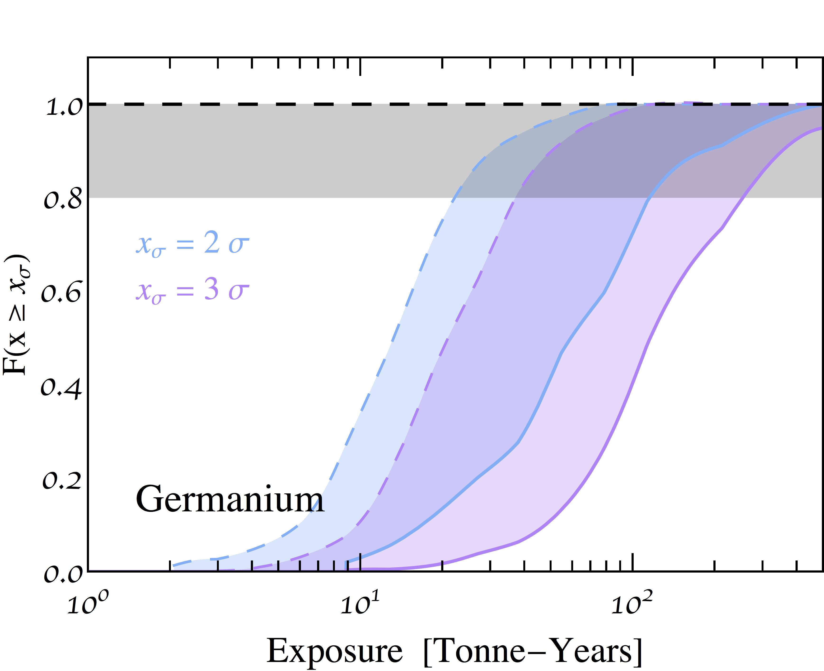
In the Fig. 6 we show the fraction of simulated data sets generated with a particular exposure MT that fulfill this requirement, for or 3. Namely, we determine the fraction of simulated data sets that produce p-values (i.e. those resulting in detection of geoneutrinos), by computing
| (20) |
where is the number of simulated data sets with fixed parameters .
Notice that the fraction is the “power” of the test of with respect to the alternative hypothesis , in which (e.g. Patrignani et al. 2016, Sec. 40), i.e. . This means that the probability of not rejecting when the “geoneutrino detection” alternative hypothesis is true is less than the value .
V.2 Results
Fig. 6 shows the two bands of fractions of simulated data sets generated with a particular exposure MT in which there is a detection of geoneutrinos at an x level with x , for =2 (in blue) and =3 (in purple), as a function of the exposure MT, for Ar, Ge and Si compositions. The higher exposure boundary (solid line) in each band assumes the systematic errors shown in Table 3. The lower exposure boundary (dashed line) of each band assumes instead a very optimistic scenario in which the errors have been divided by a factor of 100. The gray shaded area highlights the region of , where the chance of a type-2 error is small (i.e ).
With a Xe target even a 2 detection of geoneutrinos is not reachable below a 500 tonne-year exposure, the largest we consider. The reason is that for the 0.1 keV threshold that we assume only a small portion of 238U geoneutrino signal is observable (see Fig. 4).
Fig. 6 shows that the most promising detector configuration for geoneutrino detection is based on Ge, because of the lowest potential energy threshold.
VI Summary
A measurement of the level of geoneutrino emission is of utmost importance to determine the fraction of the heat emitted by Earth that remains from its formation. The major uncertainty is due to the unknown mantle contribution to the radiogenic heat.
Direct detection experiments have a clear advantage over scintillator-based experiments, which have been used to study geoneutrinos thus far, in that their threshold could be low enough (at least in Ge- and Si-based detectors) to observe geoneutrinos with energies below the kinematic threshold of 1.8 MeV, the lowest neutrino energy required for inverse beta decay. This means that 40K geoneutrinos can also contribute to the signal in direct detection experiments. A measurement of the present level of 40K with respect to the levels of other geoneutrino types could provide insight into Earth’s “volatility curve”, a central quantity for Earth’s formation history Bellini et al. 2013.
In this paper we computed the electron and nuclear recoil spectra in different target materials. In Fig. 1 one can see that the geoneutrino electron recoil rate is about one order of magnitude lower than the rate of CNO neutrinos, whose detection sensitivity has been recently explored Billard et al. 2015; Cerdeno et al. 2018; Newstead et al. 2019.
For the detection of nuclear recoils from geoneutrino signal we considered several potential experimental setups with optimistic thresholds and located in the Jinping Underground Laboratory in China, where the expected geoneutrino flux is significantly larger than in other laboratory sites, because of its proximity to the Himalayas, where the crust is the thickest. Assuming that radiogenic heat accounts for most of the heat emitted by our planet, a viable possibility, we study the minimal required exposures for a geoneutrino observation at the 2 and 3 level, if the background is due only to other neutrinos (solar and reactor neutrinos).
The results of our analysis are shown in Fig. 6. The most promising target material analyzed in this study for geoneutrino detection is germanium, which could have the lowest experimental threshold, if the exposure reaches tonne-years.
Acknowledgements
We thank Carolina Lithgow-Bertelloni, Lars Stixrude, Gerald Schubert and Linyan Wan for discussions and Sergio Palomares-Ruiz for comments. The work of GBG and VT was supported in part by the U.S. Department of Energy (DOE) under Grant No. DE-SC0009937. SJW acknowledges support from Spanish Ministry of Economy and Competitiveness (MINECO) national grants FPA2014-57816-P and FPA2017- 85985-P, and from the European projects H2020-MSCAITN-2015//674896-ELUSIVES and H2020-MSCA-RISE2015.
References
- Billard et al. (2014) J. Billard, L. Strigari, and E. Figueroa-Feliciano, Phys. Rev. D89, 023524 (2014), arXiv:1307.5458 [hep-ph] .
- Monroe and Fisher (2007) J. Monroe and P. Fisher, Phys. Rev. D76, 033007 (2007), arXiv:0706.3019 [astro-ph] .
- Gelmini et al. (2018) G. B. Gelmini, V. Takhistov, and S. J. Witte, JCAP 1807, 009 (2018), arXiv:1804.01638 [hep-ph] .
- Akimov et al. (2017) D. Akimov et al. (COHERENT), Science 357, 1123 (2017), arXiv:1708.01294 [nucl-ex] .
- Pospelov (2011) M. Pospelov, Phys. Rev. D84, 085008 (2011), arXiv:1103.3261 [hep-ph] .
- Billard et al. (2015) J. Billard, L. E. Strigari, and E. Figueroa-Feliciano, Phys. Rev. D91, 095023 (2015), arXiv:1409.0050 [astro-ph.CO] .
- Harnik et al. (2012) R. Harnik, J. Kopp, and P. A. N. Machado, JCAP 1207, 026 (2012), arXiv:1202.6073 [hep-ph] .
- Dutta et al. (2017) B. Dutta, S. Liao, L. E. Strigari, and J. W. Walker, Phys. Lett. B773, 242 (2017), arXiv:1705.00661 [hep-ph] .
- Chakraborty et al. (2014) S. Chakraborty, P. Bhattacharjee, and K. Kar, Phys. Rev. D89, 013011 (2014), arXiv:1309.4492 [astro-ph.HE] .
- Cerdeno et al. (2018) D. G. Cerdeno, J. H. Davis, M. Fairbairn, and A. C. Vincent, JCAP 1804, 037 (2018), arXiv:1712.06522 [hep-ph] .
- Essig et al. (2018) R. Essig, M. Sholapurkar, and T.-T. Yu, Phys. Rev. D97, 095029 (2018), arXiv:1801.10159 [hep-ph] .
- Newstead et al. (2019) J. L. Newstead, L. E. Strigari, and R. F. Lang, Phys. Rev. D99, 043006 (2019), arXiv:1807.07169 [astro-ph.SR] .
- McKeen and Raj (2018) D. McKeen and N. Raj, (2018), arXiv:1812.05102 [hep-ph] .
- Bellini et al. (2013) G. Bellini, A. Ianni, L. Ludhova, F. Mantovani, and W. F. McDonough, Prog. Part. Nucl. Phys. 73, 1 (2013), arXiv:1310.3732 [physics.geo-ph] .
- Hollenbach and Herndon (2001) D. F. Hollenbach and J. M. Herndon, Proc. Natl. Acad. Sci. 98, 11085 (2001).
- Araki et al. (2005) T. Araki et al., Nature 436, 499 (2005).
- Bellini et al. (2010) G. Bellini et al. (Borexino), Phys. Lett. B687, 299 (2010), arXiv:1003.0284 [hep-ex] .
- Andringa et al. (2016) S. Andringa et al. (SNO+), Adv. High Energy Phys. 2016, 6194250 (2016), arXiv:1508.05759 [physics.ins-det] .
- An et al. (2016) F. An et al. (JUNO), J. Phys. G43, 030401 (2016), arXiv:1507.05613 [physics.ins-det] .
- Han et al. (2016) R. Han, Y.-F. Li, L. Zhan, W. F. McDonough, J. Cao, and L. Ludhova, Chin. Phys. C40, 033003 (2016), arXiv:1510.01523 [physics.ins-det] .
- Cicenas and Solomey (2012) B. Cicenas and N. Solomey (HANOHANO), Proceedings, 2nd International Conference on Technology and Instrumentation in Particle Physics 2011: Chicago, Illinois, 9-14 Jun 2011, Phys. Procedia 37, 1324 (2012).
- Beacom et al. (2017) J. F. Beacom et al. (Jinping), Chin. Phys. C41, 023002 (2017), arXiv:1602.01733 [physics.ins-det] .
- Wan et al. (2017) L. Wan, G. Hussain, Z. Wang, and S. Chen, Phys. Rev. D95, 053001 (2017), arXiv:1612.00133 [hep-ex] .
- Sramek et al. (2016) O. Sramek, B. Roskovec, S. A. Wipperfurth, Y. Xi, and W. F. McDonough, Sci. Rep. 6, 33034 (2016).
- Leyton et al. (2017) M. Leyton, S. Dye, and J. Monroe, Nature Commun. 8, 15989 (2017), arXiv:1710.06724 [physics.geo-ph] .
- Wang and Chen (2017) Z. Wang and S. Chen, (2017), arXiv:1709.03743 [hep-ex] .
- Cushman et al. (2013) P. Cushman et al., in Proceedings, Snowmass, 2013 (2013) arXiv:1310.8327 [hep-ex] .
- Aprile et al. (2017) E. Aprile et al. (XENON), Phys. Rev. Lett. 119, 181301 (2017), arXiv:1705.06655 [astro-ph.CO] .
- Aprile et al. (2018) E. Aprile et al. (XENON), Phys. Rev. Lett. 121, 111302 (2018), arXiv:1805.12562 [astro-ph.CO] .
- Akerib et al. (2017) D. S. Akerib et al. (LUX), Phys. Rev. Lett. 118, 021303 (2017), arXiv:1608.07648 [astro-ph.CO] .
- Aprile et al. (2016) E. Aprile et al. (XENON), Phys. Rev. D94, 092001 (2016), [Erratum: Phys. Rev.D95,no.5,059901(2017)], arXiv:1605.06262 [astro-ph.CO] .
- Akerib et al. (2018) D. S. Akerib et al. (LUX-ZEPLIN), (2018), arXiv:1802.06039 [astro-ph.IM] .
- Agnes et al. (2018a) P. Agnes et al. (DarkSide), Phys. Rev. Lett. 121, 081307 (2018a), arXiv:1802.06994 [astro-ph.HE] .
- Agnes et al. (2018b) P. Agnes et al. (DarkSide), Phys. Rev. D98, 102006 (2018b), arXiv:1802.07198 [astro-ph.CO] .
- Agnese et al. (2017) R. Agnese et al. (SuperCDMS), Phys. Rev. D95, 082002 (2017), arXiv:1610.00006 [physics.ins-det] .
- Ludhova and Zavatarelli (2013) L. Ludhova and S. Zavatarelli, Adv. High Energy Phys. 2013, 425693 (2013), arXiv:1310.3961 [hep-ex] .
- Davies and Davies (2010) J. H. Davies and D. R. Davies, Solid Earth 1, 5 (2010).
- Sramek et al. (2013) O. Sramek, W. F. McDonough, E. S. Kite, V. Lekic, S. Dye, and S. Zhong, Earth Planet. Sci. Lett. 361, 356 (2013), arXiv:1207.0853 [physics.geo-ph] .
- Agostini et al. (2015) M. Agostini et al. (Borexino), Phys. Rev. D92, 031101 (2015), arXiv:1506.04610 [hep-ex] .
- Huang et al. (2013) Y. Huang, V. Chubakov, F. Mantovani, R. L. Rudnick, and W. F. McDonough, ArXiv e-prints (2013), arXiv:1301.0365 [physics.geo-ph] .
- Haxton et al. (2013) W. C. Haxton, R. G. Hamish Robertson, and A. M. Serenelli, Ann. Rev. Astron. Astrophys. 51, 21 (2013), arXiv:1208.5723 [astro-ph.SR] .
- Grevesse and Sauval (1998) N. Grevesse and A. J. Sauval, Space Sci. Rev. 85, 161 (1998).
- Asplund et al. (2009) M. Asplund, N. Grevesse, A. J. Sauval, and P. Scott, Ann. Rev. Astron. Astrophys. 47, 481 (2009), arXiv:0909.0948 [astro-ph.SR] .
- Hayes and Vogel (2016) A. C. Hayes and P. Vogel, Ann. Rev. Nucl. Part. Sci. 66, 219 (2016), arXiv:1605.02047 [hep-ph] .
- Ma et al. (2013) X. B. Ma, W. L. Zhong, L. Z. Wang, Y. X. Chen, and J. Cao, Phys. Rev. C88, 014605 (2013), arXiv:1212.6625 [nucl-ex] .
- Murayama and Pierce (2002) H. Murayama and A. Pierce, Phys. Rev. D65, 013012 (2002), arXiv:hep-ph/0012075 [hep-ph] .
- Baldoncini et al. (2015) M. Baldoncini, I. Callegari, G. Fiorentini, F. Mantovani, B. Ricci, V. Strati, and G. Xhixha, Phys. Rev. D91, 065002 (2015), arXiv:1411.6475 [physics.ins-det] .
- (48) “U.S. Energy Information Administration,” https://www.eia.gov/todayinenergy/detail.php?id=1490.
- Kopeikin (2012) V. I. Kopeikin, Phys. Atom. Nucl. 75, 143 (2012), [Yad. Fiz.75N2,165(2012)].
- Vogel and Engel (1989) P. Vogel and J. Engel, Phys. Rev. D39, 3378 (1989).
- Mueller et al. (2011) T. A. Mueller et al., Phys. Rev. C83, 054615 (2011), arXiv:1101.2663 [hep-ex] .
- Huber (2011) P. Huber, Phys. Rev. C84, 024617 (2011), [Erratum: Phys. Rev.C85,029901(2012)], arXiv:1106.0687 [hep-ph] .
- Adey et al. (2018) D. Adey et al. (Daya Bay), (2018), arXiv:1808.10836 [hep-ex] .
- Vogel et al. (1981) P. Vogel, G. K. Schenter, F. M. Mann, and R. E. Schenter, Phys. Rev. C24, 1543 (1981).
- Schreckenbach et al. (1985) K. Schreckenbach, G. Colvin, W. Gelletly, and F. Von Feilitzsch, Phys. Lett. 160B, 325 (1985).
- Von Feilitzsch et al. (1982) F. Von Feilitzsch, A. A. Hahn, and K. Schreckenbach, Phys. Lett. 118B, 162 (1982).
- Hahn et al. (1989) A. A. Hahn, K. Schreckenbach, G. Colvin, B. Krusche, W. Gelletly, and F. Von Feilitzsch, Phys. Lett. B218, 365 (1989).
- Freedman et al. (1977) D. Z. Freedman, D. N. Schramm, and D. L. Tubbs, Ann. Rev. Nucl. Part. Sci. 27, 167 (1977).
- Helm (1956) R. H. Helm, Phys. Rev. 104, 1466 (1956).
- Patrignani et al. (2016) C. Patrignani et al. (Particle Data Group), Chin. Phys. C40, 100001 (2016).
- Chen et al. (2014a) J.-W. Chen, H.-C. Chi, K.-N. Huang, C. P. Liu, H.-T. Shiao, L. Singh, H. T. Wong, C.-L. Wu, and C.-P. Wu, Phys. Lett. B731, 159 (2014a), arXiv:1311.5294 [hep-ph] .
- Chen et al. (2014b) J.-W. Chen, H.-C. Chi, H.-B. Li, C. P. Liu, L. Singh, H. T. Wong, C.-L. Wu, and C.-P. Wu, Phys. Rev. D90, 011301 (2014b), arXiv:1405.7168 [hep-ph] .
- Chen et al. (2015) J.-W. Chen, H.-C. Chi, K.-N. Huang, H.-B. Li, C. P. Liu, L. Singh, H. T. Wong, C.-L. Wu, and C.-P. Wu, Phys. Rev. D91, 013005 (2015), arXiv:1411.0574 [hep-ph] .
- Chen et al. (2017) J.-W. Chen, H.-C. Chi, C. P. Liu, and C.-P. Wu, Phys. Lett. B774, 656 (2017), arXiv:1610.04177 [hep-ex] .
- de Salas et al. (2018) P. F. de Salas, D. V. Forero, C. A. Ternes, M. Tortola, and J. W. F. Valle, Phys. Lett. B782, 633 (2018), arXiv:1708.01186 [hep-ph] .
- Agostini et al. (2018) M. Agostini et al. (BOREXINO), Nature 562, 505 (2018).
- Cowan et al. (2011a) G. Cowan, K. Cranmer, E. Gross, and O. Vitells, Eur. Phys. J. C71, 1554 (2011a), [Erratum: Eur. Phys. J.C73,2501(2013)], arXiv:1007.1727 [physics.data-an] .
- Rolke et al. (2005) W. A. Rolke, A. M. Lopez, and J. Conrad, Nucl. Instrum. Meth. A551, 493 (2005), arXiv:physics/0403059 [physics] .
- Cowan et al. (2011b) G. Cowan, K. Cranmer, E. Gross, and O. Vitells, (2011b), arXiv:1105.3166 [physics.data-an] .
- Billard et al. (2012) J. Billard, F. Mayet, and D. Santos, Phys. Rev. D85, 035006 (2012), arXiv:1110.6079 [astro-ph.CO] .
- Aprile et al. (2011) E. Aprile et al. (XENON100), Phys. Rev. D84, 052003 (2011), arXiv:1103.0303 [hep-ex] .
- Ruppin et al. (2014) F. Ruppin, J. Billard, E. Figueroa-Feliciano, and L. Strigari, Phys. Rev. D90, 083510 (2014), arXiv:1408.3581 [hep-ph] .