Natural $\alpha$-Attractors from ${\cal N}=1$ Supergravity via flat Kähler Manifolds

We start by defining a Kähler potential of the form

$$K=-\frac{3\alpha}{8}\log^{2}\left[\frac{\left(1+\Phi\right)\left(1-\Phi^{*}\right)}{\left(1-\Phi\right)\left(1+\Phi^{*}\right)}\right]+SS^{*}-\zeta(SS^{*})^{2}$$

(10)

where $\Phi$ is the inflaton superfield (non-canonical) and $S$ is the chiral multiplet which serves the job of the stabilizer field or the nilpotent superfield. During inflation, the inflaton partner $\Phi-\Phi^{*}$ and the stabilizer field attains zero vev and hence the Kähler potential vanishes. This is obviously due to the inflaton shift symmetry in the Kähler potential and this shift symmetry is explicitly visible when one writes the above Kähler potential in its series form as

$$K=-\left[\sum_{\begin{subarray}{c}n=odd\end{subarray}}^{N}K^{(n)}\left(\Phi^{n}-\Phi^{*n}\right)\right]^{2}+SS^{*}-\zeta(SS^{*})^{2}$$

(11)

with

$$K^{(n)}=\frac{1}{n}\sqrt{\frac{3\alpha}{2}},\penalty\ \penalty\ \penalty\ \penalty\ \penalty\ \penalty\ \penalty\ \penalty\ \penalty\ \penalty\ N\rightarrow\infty.$$

(12)

The index $n$ takes only odd positive integer values and $K^{(n)}$ are the dimensionless coupling constants for the self interactions of chiral superfields. This Kähler potential is invariant under the following shift transformation:

$$\sum_{\begin{subarray}{c}n=odd\end{subarray}}^{N}K^{(n)}\Phi^{n}\rightarrow\sum_{\begin{subarray}{c}n=odd\end{subarray}}^{N}K^{(n)}\Phi^{n}+C_{N}$$

(13)

Because of the invariance (13), one can consider $\sum_{\begin{subarray}{c}n=odd\end{subarray}}^{N}K^{(n)}\Phi^{n}$ as a composite field $\hat{\Phi}$, which transforms under a Nambu-Goldstone like shift symmetry. This shift symmetry generalizes the shift symmetries proposed in kawasaki2000naturalchaotic; linear_running_kinetic_inflation_takahashi; running_kinetic_inflation_takahashi in the context of supergravity realization of the chaotic inflation and running kinetic inflation. Due to this shift symmetry, the real component of the composite field $\hat{\Phi}$ will be absent in the Kähler potential (11), and this real component $Re\left[\sum_{\begin{subarray}{c}n=odd\end{subarray}}^{N}K^{(n)}\Phi^{n}\right]=Re\left[\hat{\Phi}\right]$ can be identified as the inflaton scalar field linear_running_kinetic_inflation_takahashi; running_kinetic_inflation_takahashi. Since physics is invariant under field transformation, one can also proceed the same analysis in terms of the real non-canonical variables. In such a scenario, real part of $\Phi$ can be identified as inflaton in terms of the non-canonical chiral field $\Phi$. In order to explicitly show that the non-canonical kinetic term arising from this model also has a pole of order two with respect to the real field variable, we continue our investigation in terms of the non-canonical variables from the Kähler potential defined in (10). This investigation and the subsequent analysis based on the series Kähler potential (11) is relegated to Appendix A. The Kähler potential defined in (10) can give the following kinetic term for inflation

$$\frac{1}{\sqrt{-g}}L_{kin}=-\frac{3\alpha}{\left(1-\Phi^{2}\right)\left(1-\Phi^{*2}\right)}\partial_{\mu}\Phi\partial^{\mu}\Phi^{*}\\ -\left(1-4\zeta S^{*}S\right)\partial_{\mu}S\partial^{\mu}S^{*}$$

(14)

As in the traditional way, we also consider a small breaking term of the shift symmetry in the superpotential,

$$W=mS\Phi$$

(15)

for the successful inflation. This small breaking term ensures a tree-level mass for the field $\Phi$ through F-term of the stabilizer field $S$. When $m\rightarrow 0$, we have an enhanced shift symmetry so that our model is natural according to ’t Hooft’s sense t.hooft_natural. The superpotential considered in (15) is completely reserved for the construction of T-model of $\alpha$- attractors. However, to construct a general $\alpha$-attractor model, one can also define a superpotential of the form,

$$W=mSf(\Phi)$$

(16)

where $f(\Phi)$ is the general function of the chiral superfield $\Phi$. Now, let us decompose these complex chiral superfields $\Phi$ and $S$ into real scalar fields

$$\Phi=\frac{1}{\sqrt{6\alpha}}\left(\phi+i\chi\right),\penalty\ \penalty\ \penalty\ \penalty\ \penalty\ \penalty\ \penalty\ \penalty\ \penalty\ S=\frac{1}{\sqrt{2}}\left(s+i\beta\right)$$

(17)

Based on the F-term potential of ${\cal N}=1$ SUGRA,

$$V=e^{K}\left(D_{\Phi_{i}}WK^{ij^{*}}D_{\Phi_{j^{*}}}W^{*}-3\left|W\right|^{2}\right).$$

(18)

and with the kinetic term (14), one will end up with the total Lagrangian for the inflation real field $\phi$ along the inflationary trajectory $\chi=s=\beta=0$ as

$$L=\sqrt{-g}\left[\frac{1}{2}R-\frac{1}{\left(1-\frac{\phi^{2}}{6\alpha}\right)^{2}}\frac{1}{2}\partial_{\mu}\phi\partial^{\mu}\phi-V(\phi)\right]$$

(19)

with

$$V(\phi)=\begin{cases}m^{2}\frac{\phi^{2}}{6\alpha},&\text{for }W=mS\Phi\\ m^{2}f^{2}(\frac{\phi}{\sqrt{6\alpha}}),&\text{for }W=mSf(\Phi).\end{cases}$$

(20)

The Lagrangian (19) with (20) defines the complete $\alpha$-attractor model for inflation in terms of non-canonical real field variable $\phi$.

Next, we study the stability of the inflationary trajectory with respect to the small fluctuations of the fields $\chi$ and $S$. In order to check this stability, one can calculate the canonical masses of all the fields orthogonal to the inflaton direction $\phi$ based on the F-term potential of SUGRA (18) for the theory (10) with (15) or (16) at $\chi=S=0$ as¹¹ 1 It is well known that, due to the shift symmetry (13) in terms of its canonical composite variables $\hat{\Phi}$, $m_{\text{Im}(\hat{\Phi})}>\mathcal{O}(H)$ for any choice of the superpotential Kallosh2010general_inflaton_pot_in_supergravity_stabilizerfield=sGoldstino. Since physics is invariant under the field transformation, it is well expected that the canonical mass of non-canonical field $m_{\chi}>\mathcal{O}(H)$. However, we provide the explicit calculations for the same here.

$$m_{\chi}^{2}=6H^{2}\left(1+\epsilon-\eta/2\right)$$

(21)

$$m_{\beta}^{2}=m_{s}^{2}=12H^{2}\left(\zeta+\epsilon/4\right)$$

(22)

and the canonical mass of the inflaton is

$$m_{\phi}^{2}=3H^{2}\eta$$

(23)

Here we have used $V(\phi)=3H^{2}$ where H is the Hubble’s constant, and $\epsilon$ and $\eta$ are the slow-roll parameters of inflation in terms of non-canonical variable $\phi$. In order to get the canonical masses for both inflaton $\phi$ and its partner $\chi$, we have multiplied by the factor $\left(1-\phi^{2}/6\alpha\right)^{2}$ to the second derivatives of their potentials. From (21) it is evident that for any value of $\alpha$, $m_{\chi}>\mathcal{O}(H)$, i.e., the field $\chi$ is heavy and reaches its minimum quickly. Moreover from (22), for $\zeta\geq 1/12$, $m_{s}=m_{\beta}>\mathcal{O}(H)$, is also heavy and vanish. Therefore, during inflation all these fields are stabilized at the inflationary trajectory $\chi=S=0$.

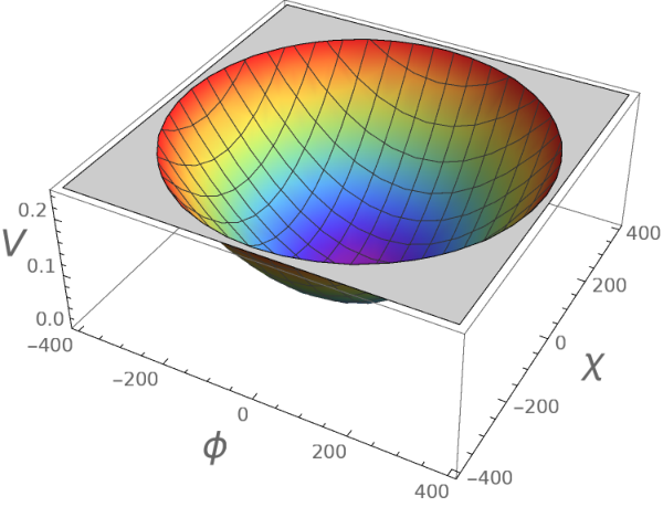
Now, we focus on the properties of supergarvity potential (18) based on our model. For the simplest case, we consider T-model potential based on (10) and (15) in terms of the non-canonical real variables $\Phi=(\phi+i\chi)/\sqrt{6\alpha}$. From Fig.(1), it is evident that existence of flat direction is not visible in terms of these non-canonical variables $\phi$ and $\chi$ for the theory (10) and (15) due to the existence of the non-canonical kinetic term in it. In order to see the flat direction explicitly in the potential, we have to switch to more suitable variables, say, canonical variables for both $\phi$ and $\chi$ fields. So we will use the variables $\hat{\Phi}=(\psi+i\theta)\sqrt{6\alpha}$, which is related to $\Phi$ as $\Phi=\tanh\hat{\Phi}$. In terms of this new variables kinetic terms for both the fields are canonical, i.e.,

$$L_{kin}=\frac{1}{2}\left(d\psi^{2}+d\theta^{2}\right)$$

(24)

for any values of both $\psi$ and $\theta$. Further, the potential (18) at $S=0$ takes the form

$$V=m^{2}e^{\frac{\theta}{\alpha}}\left|\tanh\frac{\psi+i\theta}{\sqrt{6\alpha}}\right|^{2}\\ =m^{2}\frac{\cosh\sqrt{\frac{2}{3\alpha}}\psi-\cos\sqrt{\frac{2}{3\alpha}}\theta}{\cosh\sqrt{\frac{2}{3\alpha}}\psi+\cos\sqrt{\frac{2}{3\alpha}}\theta}e^{\frac{\theta^{2}}{\alpha}}$$

(25)

This potential is depicted in the Fig.(2), which is the three dimensional plot of T-model potential with symmetric shoulders and visible flat directions. One can see that this scalar potential has a Minkowski minimum at small values of the inflaton field $\psi$ and has infinitely long dS valley at large values of $\psi$ with constant depth and width. Thus, this potential closely resembles to the one obtained from the theory based on the hyperbolic geometry of $\alpha$-attractors cosmo_attracts_nd_initial_cond_for_inflation.

Finally, we focus on the most important part of our model, which is the geometry of the Kähler manifold. It is quiet evident that because of the shift symmetry (13) of the Kähler potential (11), Kähler manifold is flat in terms of its canonical variables. More clearly, due to the shift symmetry, the series Kähler potential attains a canonical form in terms of its composite canonical fields $\hat{\Phi}=\sum_{\begin{subarray}{c}n=odd\end{subarray}}^{N}K^{(n)}$ given by

$$K=k\left(\hat{\Phi}-\hat{\Phi}^{*}\right)^{2}+SS^{*}-\zeta(SS^{*})^{2}$$

(26)

where $k$ is some arbitrary constant. As an another example, one can also write the Kähler potential (10) in a more convenient form as

$$K=-\frac{3\alpha}{2}\left(\tanh^{-1}\Phi-\tanh^{-1}\Phi^{*}\right)^{2}+SS^{*}-\zeta(SS^{*})^{2}.$$

(27)

This Kähler potential is also invariant under the following shift symmetric transformation:

$$\tanh^{-1}\Phi\rightarrow\tanh^{-1}\Phi+C$$

(28)

In this case, we choose composite canonical field $\hat{\Phi}=\tanh^{-1}\Phi$. This is why we obtained canonical kinetic terms for both $\psi$ and $\theta$ fields with an infinite dS valley potential earlier with these composite fields (see 24 and 25). In terms of this canonical field $\hat{\Phi}$, the above Kähler potential takes the same form as (26) which is the well known Kähler potential proposed in kawasaki2000naturalchaotic with flat Kähler geometry. Thus, our Kähler manifold is also flat in terms of its canonical variables. As physics is invariant under field transformation, we expect same for non-canonical variables as well. However, we explicitly calculate the curvature for Kähler manifold in terms of its non-canonical variable $\Phi$ from the Kähler potential (10). Based on this Kähler potential, metric of the moduli space is defined as

$$ds^{2}=g_{\Phi\Phi^{*}}d\Phi d\Phi^{*}$$

(29)

where

$$g_{\Phi\Phi^{*}}=K_{\Phi\Phi^{*}}=\frac{3\alpha}{\left(1-\Phi^{2}\right)\left(1-\Phi^{*2}\right)}.$$

(30)

Now, we proceed to compute the non-vanishing Levi-Civita connection coefficients, Riemannian tensors, and the curvature of the moduli space associated with this Kähler metric. They are given as

$$\Gamma_{\Phi\Phi}^{\Phi}=\frac{2\Phi}{\left(1-\Phi^{2}\right)},\penalty\ \penalty\ \penalty\ \penalty\ \penalty\ \penalty\ \penalty\ \penalty\ \Gamma_{\Phi^{*}\Phi^{*}}^{\Phi^{*}}=\frac{2\Phi^{*}}{\left(1-\Phi^{*2}\right)},$$

(31)

$$\mathcal{R}_{\Phi\Phi^{*}\Phi}^{\Phi}=\partial_{\Phi^{*}}\Gamma_{\Phi\Phi}^{\Phi}=0.$$

(32)

Since all components of these Riemannian tensors vanish, curvature of the Kähler manifold is $\mathcal{R}_{\text{K\"{a}hler}}=0$. Alternatively, from the definition of curvature of Kähler manifold via the metric:

$$\mathcal{R}_{\text{K\"{a}hler}}=-g_{\Phi\Phi^{*}}^{-1}\partial_{\Phi}\partial_{\Phi^{*}}\log g_{\Phi\Phi^{*}}=0.$$

(33)

From the above, we conclude that geometry associated with our Kähler manifold is flat.

So far, we have $\alpha$-attractor models in supergravity based on the hyperbolic Kähler geometry of the Poincaré disk or half plane with the logarithmic Kähler potentials. This logarithmic Kähler potential is the signature of the hyperbolic Kähler geometry of those models. In such models, parameter $\alpha$ is interpreted as the reciprocal of the curvature of the Kähler manifold. In contrast, we present an $\alpha$-attractor model based on the square of the logarithmic Kähler potential with a vanishing curvature. However, this leaves us with the following question - how can we interpret the parameter $\alpha$? Without going into the further details of Kähler geometry, from (12), a possible interpretation is that the parameter $\alpha$ plays the roll of coupling constants, which represents the self interaction of the inflaton superfields. For a non-canonically normalized field $\Phi=(\phi+i\chi)/\sqrt{2}$, (12) can be modified as

$$K^{(n)}=\frac{1}{(6\alpha)^{\frac{n-1}{2}}}\frac{\left(\sqrt{2}\right)^{n-2}}{n}$$

(34)

Bahaviour of these coupling constants under different values of $\alpha$ is shown in Fig.(3).

In this section, we consider the Kähler potential for the chiral superfield $\Phi$ as

$$K=-\frac{3\alpha}{8}\log^{2}\left[\frac{\left(1+\Phi^{2}\right)\left(1-\Phi^{*2}\right)}{\left(1-\Phi^{2}\right)\left(1+\Phi^{*2}\right)}\right]+SS^{*}-\zeta(SS^{*})^{2}$$

(35)

This Kähler potential also has a shift symmetry in terms of its canonical composite chiral fields given by $\hat{\Phi}=\sum_{\begin{subarray}{c}n=odd\end{subarray}}^{N}K^{(2n)}\Phi^{2n}$. More explicitly, we write the above Kähler potential in the following form:

$$K=-\left[\sum_{\begin{subarray}{c}n=odd\end{subarray}}^{N}\frac{K^{(2n)}}{M_{pl}^{2n-2}}\left(\Phi^{2n}-\Phi^{*2n}\right)\right]^{2}\\ +SS^{*}-\zeta(SS^{*})^{2}$$

(36)

which is invariant under the following transformation

$$\sum_{\begin{subarray}{c}n=odd\end{subarray}}^{N}K^{(2n)}\Phi^{2n}\rightarrow\sum_{\begin{subarray}{c}n=odd\end{subarray}}^{N}K^{(2n)}\Phi^{2n}+C_{N}.$$

(37)

We also consider a shift symmetry breaking superpotential

$$W=\sqrt{\lambda}S\Phi^{2}$$

(38)

or generally,

$$W=Sf(\Phi^{2}).$$

(39)

One may see that this model is related to the previous model (11) and (15) (or (16)) by a scaled transformation in the field $\Phi\rightarrow\Phi^{2}$. Since this scaling is non-linear and these models are not related by any Kähler transformations, one can consider these as two different models. The Kähler potential defined in (35) produces the following kinetic term as

$$\frac{1}{\sqrt{-g}}L_{kin}=-\frac{12\alpha}{\left(1-\Phi^{4}\right)\left(1-\Phi^{*4}\right)}\partial_{\mu}\Phi\partial^{\mu}\Phi^{*}\\ -\left(1-4\zeta S^{*}S\right)\partial_{\mu}S\partial^{\mu}S^{*}$$

(40)

decomposing these complex variables into real variables as follows

$$\Phi=\frac{1}{(6\alpha)^{\frac{1}{4}}}\left(\phi+i\chi\right),\penalty\ \penalty\ \penalty\ \penalty\ \penalty\ \penalty\ \penalty\ \penalty\ \penalty\ S=\frac{1}{\sqrt{2}}\left(s+i\beta\right).$$

(41)

With the help of (18), for the theory (40) and (38) (or 39), one can write the total Lagrangian for inflation along $S=\chi=0$ as

$$L=\sqrt{-g}\left[\frac{1}{2}R-\frac{4\phi^{2}}{\left(1-\frac{\phi^{4}}{6\alpha}\right)^{2}}\frac{1}{2}\partial_{\mu}\phi\partial^{\mu}\phi-V(\phi)\right]$$

(42)

where

$$V=\begin{cases}\frac{\lambda}{6\alpha}\phi^{4},&\text{for }W=\sqrt{\lambda}S\Phi\\ f^{2}\left(\frac{\phi^{2}}{\sqrt{6\alpha}}\right),&\text{for }W=Sf(\Phi^{2}).\end{cases}$$

(43)

Note that the kinetic term has four poles of order two at $((6\alpha)^{\frac{1}{4}},-(6\alpha)^{\frac{1}{4}},i(6\alpha)^{\frac{1}{4}},-i(6\alpha)^{\frac{1}{4}})$ and has a leading pole of order two with residue $\frac{3}{2}\alpha$. This is the required condition in kinetic term for the $\alpha$-attractors in its non-canonical variables so that the observational predictions are to a large extent determined by this term, rather than by the potential. In order to switch to the canonical variable, we solve the equation

$$\frac{2\phi}{\left(1-\frac{\phi^{2}}{6\alpha}\right)}\partial\phi=\partial\psi$$

(44)

which gives

$$\phi=\left(6\alpha\right)^{\frac{1}{4}}\tanh^{\frac{1}{2}}\left(\frac{\psi}{\sqrt{6\alpha}}\right)$$

(45)

Thus, the total Lagrangian for the $\alpha$-attractor model in terms of canonical variable $\psi$ reads

$$L=\sqrt{-g}\left[\frac{1}{2}R-\frac{1}{2}\partial_{\mu}\psi\partial^{\mu}\psi-f^{2}\left(\tanh\left(\frac{\psi}{\sqrt{6\alpha}}\right)\right)\right].$$

(46)

Masses of all stabilized heavy fields along inflationary trajectory $S=\chi=0$ are given by

$$m_{\chi}^{2}=6H^{2}\left(1-\frac{3}{4}\epsilon+\eta/2\right)$$

(47)

and

$$m_{\beta}^{2}=m_{s}^{2}=12H^{2}\left(\zeta+\epsilon/8\right).$$

(48)

These masses are slightly different compared to the masses of Model-I. The scalar potential for the model (36) and (38) in terms of the variables (41) is shown in Fig.(4). As in the earlier case, here also the flat directions are not visible in terms of these variables. Migrating to more adequate variables $\Phi=\tanh^{1/2}\hat{\Phi}$ with $\hat{\Phi}=(\psi+i\theta)\sqrt{6\alpha}$, we get exactly the same potential (25) that we obtained in the previous model, which has visible flat directions. It is shown in Fig.(2). Moreover, the kinetic term is canonical for inflaton and its partner (see 24).

Finally, the metric of the moduli space obtained from the Kähler potential (35),

$$ds^{2}=\frac{12\alpha}{\left(1-\Phi^{4}\right)\left(1-\Phi^{*4}\right)}d\Phi d\Phi^{*}$$

(49)

gives non-vanishing connection coefficients as follows:

$$\Gamma_{\Phi\Phi}^{\Phi}=\frac{1+3\Phi^{4}}{\Phi\left(1-\Phi^{4}\right)},\penalty\ \penalty\ \penalty\ \penalty\ \penalty\ \penalty\ \penalty\ \penalty\ \Gamma_{\Phi^{*}\Phi^{*}}^{\Phi^{*}}=\frac{1+3\Phi^{*4}}{\Phi^{*}\left(1-\Phi^{*4}\right)}.$$

(50)

However, all components of Riemannian tensors vanish and hence, the geometry of the Kähler manifold is flat. As before, the parameter $\alpha$ here can be related to the coupling constants as

$$K^{(2n)}=\frac{2^{n-1}}{n}\frac{1}{(6\alpha)^{\frac{n-1}{2}}}$$

(51)

and its behaviour is shown in Fig.(5).

References

- (1) R. Kallosh and A. Linde, Universality Class in Conformal Inflation, JCAP 1307 (2013) 002, [arXiv:1306.5220 [hep-th]]
- (2) R. Kallosh and A. Linde, Multi-field Conformal Cosmological Attractors, JCAP 1312 (2013) 006, [arXiv:1309.2015 [hep-th]]
- (3) R. Kallosh and A. Linde, Non-minimal Inflationary Attractors, JCAP 1310 (2013) 033 [arXiv:1307.7938 [hep-th]]
- (4) M. Galante, R. Kallosh, A. Linde, D. Roest, The Unity of Cosmological Attractors, Phys.Rev.Lett. 114 (2015) no.14, 141302, [arXiv:1412.3797 [hep-th]]
- (5) R. Kallosh, A. Linde, D. Roest, Superconformal Inflationary -Attractors, JHEP 1311 (2013) 198, [arXiv:1311.0472 [hep-th]]
- (6) R. Kallosh and A. Linde, Escher in the Sky, Comptes Rendus Physique 16 (2015) 914-927, [arXiv:1503.06785 [hep-th]]
- (7) D.Roest, M. Scalisi, Cosmological Attractors from -Scale Supergravity, Phys.Rev. D92 (2015) 043525, [arXiv:1503.07909 [hep-th]]
- (8) J. J. M. Carrasco, R. Kallosh, A. Linde, D. Roest, The Hyperbolic Geometry of Cosmological Attractors, Phys.Rev. D92 (2015) no.4, 041301, [arXiv:1504.05557 [hep-th]]
- (9) A. Linde Single-field -attractors, JCAP 1505 (2015) 003 [arXiv:1504.00663 [hep-th]]
- (10) Sergio Ferrara and Renata Kallosh, Seven-Disk Manifold, alpha-attractors and B-modes, Phys.Rev. D94 (2016) no.12, 126015, [arXiv:1610.04163 [hep-th]]
- (11) R. Kallosh, A. Linde, T. Wrase, Y. Yamada, Maximal Supersymmetry and B-Mode Targets, JHEP 1704 (2017) 144, [arXiv:1704.04829 [hep-th]]
- (12) A. Achúcarro, R. Kallosh, A. Linde, D. Wang, Y. Welling, Universality of multi-field -attractors, JCAP 1804 (2018) no.04, 028, [arXiv:1711.09478 [hep-th]]
- (13) A. Linde, D. Wang, Y. Welling, Y. Yamada, A. Achucarro, Hypernatural inflation, JCAP 1807 (2018) no.07, 035, [arXiv:1803.09911 [hep-th]]
- (14) M. Scalisi, Cosmological -Attractors and de Sitter Landscape, JHEP 1512 (2015) 134, [arXiv:1506.01368 [hep-th]]
- (15) M. Dias, J. Frazer, A. Retolaza, M. Scalisi, A. Westphal, Pole N-flation, [arXiv:1805.02659 [hep-th]]
- (16) Planck Collaboration, P. A. R. Ade et al., Planck 2015 results. XX. Constraints on inflation, Astron.Astrophys. 594 (2016) A20, [arXiv:1502.02114 [astro-ph.CO]]
- (17) Planck Collaboration, Y. Akrami et al., Planck 2018 results. X. Constraints on inflation, [ arXiv:1807.06211 [astro-ph.CO]]
- (18) T. Pinhero and S. Pal, Non-canonical Conformal Attractors for Single Field Inflation [arXiv:1703.07165 [hep-th]]
- (19) T. Pinhero and S. Pal, A New Class of Non-canonical Conformal Attractors for Multifield Inflation, [arXiv:1810.12712 [hep-th]]
- (20) M. Kawasaki, M. Yamaguchi, T. Yanagida, Natural Chaotic Inflation in Supergravity, Phys.Rev.Lett. 85 (2000) 3572-3575, [arXiv:hep-ph/0004243]
- (21) F. Takahashi, Linear Inflation from Running Kinetic Term in Supergravity , Phys.Lett. B693 (2010) 140-143, [arXiv:1006.2801 [hep-ph]]
- (22) K. Nakayama and F. Takahashi, Running Kinetic Inflation, JCAP 1011 (2010) 009, [arXiv:1008.2956 [hep-ph]]
- (23) G. ’t Hooft, Recent Developments in Gauge Theories, edited by G. ’t Hooft et al. (Plenum Press, Cargése, 1980),
- (24) R. Kallosh, A. Linde, T. Rube, General inflaton potentials in supergravity, Phys.Rev.D83:043507,2011, [arXiv:1011.5945 [hep-th]]
- (25) J. J. M. Carrasco, R. Kallosh, A. Linde, Cosmological Attractors and Initial Conditions for Inflation, Phys.Rev. D92 (2015) no.6, 063519, [arXiv:1506.00936 [hep-th]]