Image Segmentation Based on Multiscale Fast Spectral Clustering

This section gives a brief introduction to K-way Normalized cut (Ncut) proposed by Shi et al. [18]. Suppose image $I$ contains pixels $v_{1}\textrm{,}\ldots\textrm{,}v_{n}$, and the similarity matrix of image $I$ is the matrix $W=(w_{ij})_{n\times n}$, in which $w_{ij}$ denotes the similarity between pixel $v_{i}$ and pixel $v_{j}$ [23]. According to T. Cour et al. [19], $w_{ij}$ is defined as follows:

where

where $X_{i}$ and $Z_{i}$ denote the location and intensity of pixel $v_{i}$; $r$ denotes graph connection radius; $\sigma_{x}$ and $\sigma_{I}$ are scaling parameters; $Edge(x)$ is the edge strength at location $x$; $line(i\textrm{,}j)$ is the straight line connecting pixels $v_{i}$ and $v_{j}$ [19]. If the straight line connecting the two pixels does not cross the edge of the image, the value of $w_{C}$ will be large, reflecting that the affinity of the two pixels is high. With the similarity matrix $W$, K-way Ncut clusters the image into $k$ clusters $C=\{C_{1}\textrm{,}\;C_{2}\textrm{,}...\textrm{,}C_{k}\}$ by solving the following minimization problem [18], [24], [25]:

where

where $\bar{C_{i}}=C-C_{i}$ represents the complement of $C_{i}$; $cut(C_{i}\textrm{,}\bar{C_{i}})=\sum\limits_{v_{i}\in{C_{i}}\textrm{,}v_{j}\notin{C_{i}}}w_{ij}$ reflects the connectivity strength between $C_{i}$ and other clusters; $vol(C_{i})$ $(i=1\textrm{,}...\textrm{,}n)$ is the regularization term preventing the clustering result from being an isolated pixel.

To solve the above problem, the matrix $X=(x_{ij})_{n\times k}$ is defined as follows:

It is easy to verify $x_{j}^{T}(D-W)x_{j}=\frac{cut(C_{j}\textrm{,}\bar{C_{j}})}{vol(C_{j})}$ and $X^{T}DX=E$, where $E$ is an identity matrix and the degree matrix $D$ is defined as the diagonal matrix whose entry is $d_{i}=\sum_{j}^{n}w_{ij}$, degree of $v_{i}$.

Next, the unnormalized graph Laplacian $L$ is defined as follows:

With matrices $X$ and $L$, the minimization problem in Eq. (2) can be rewritten as the following problem:

Then, relaxing the discreteness condition and substituting $Y=D^{\frac{1}{2}}X$, the following relaxed problem is obtained :

where

is a normalized graph Laplacian. Eq. (6) is the standard form of a trace minimization problem. The Rayleigh-Ritz theorem [26] tells us that its solution is the matrix whose columns are the first $k$ eigenvectors of matrix $L_{N}$ (By “the first k eigenvectors” we refer to the eigenvectors corresponding to the k smallest eigenvalues). Also, it is obvious that solution $X$ consists of the first $k$ generalized eigenvectors of $Lu=\lambda Du$ [24].

The algorithm of normalized spectral clustering by Shi and Malik [18] is presented in Algorithm 1. Its computational complexity is $O(n^{\frac{3}{2}})$; its memory cost is $O(n)$.

Quad-tree is a widely used tree data structure in the field of image segmentation [28, 29, 30, 31, 32], and it is a spatial search tree in which each internal node has exactly four child nodes. It is the two-dimensional analog of octrees. Quad-tree decomposition divides a square image into four equal-sized square blocks, and tests each block to see if it meets some criterion of homogeneity. If a block meets the criterion, it is not divided any further. Otherwise, it is subdivided again into four blocks. This process is repeated iteratively until each block meets the criterion. The final result includes multiple sizes of blocks.

The typical criterion is as follows:

where $\Omega$ represents an image block, $var(\Omega)$ the variance of the pixel intensities of $\Omega$ and $t$ the threshold of quad-tree decomposition. Note that image $I$ can be divided into $\frac{1}{2}\log n$ levels at most [28]. Fig.1 shows the structure of a quad-tree.

In this section, we give a detailed introduction to FSC. It focuses on the spectral clustering at superpixel level. Suppose image $I$ is composed of $m$ superpixels, i.e., $I=\displaystyle\bigcup_{i=1}^{m}A_{i}$, where $A_{i}$ is the $i$-th superpixel and the number of superpixels $m$ is much smaller than the number of pixels $n$. In FSC, we treat the leaf node blocks of the quad-tree as superpixels. Next, we start to solve the problem of spectral image segmentation based on superpixels with FSC. This problem is to divide the set of superpixels into $k$ clusters $B=\{B_{1}\textrm{,}...\textrm{,}B_{k}\}$. Analogous to Ncut, the problem is equivalent to the following minimization problem:

where $FSC(B_{1}\textrm{,}B_{2}\textrm{,}...\textrm{,}B_{k})$ is defined as:

and

where $|A_{i}|$ is the number of pixels in superpixel $A_{i}$, and $cut(A_{i}\textrm{,}A_{j})=\displaystyle\sum_{v_{i}\in{A_{i}}\textrm{,}v_{j}\in A_{j}}w_{ij}$. In order to solve the problem defined in Eq. (9), the unnormalized graph Laplacian based on superpixels and the indicator vector of cluster $B_{j}$ $(j=1\textrm{,}2\textrm{,}...\textrm{,}k)$ are required. First, to construct the unnormalized graph Laplacian based on superpixels, define the indicator vector of superpixel $A_{j}$ $(j=1\textrm{,}2\textrm{,}...\textrm{,}m)$ as $h_{j}=(h_{1j}\textrm{,}h_{2j}\textrm{,}...\textrm{,}h_{nj})^{T}$ by

$\qquad{}\qquad{}\qquad{}\qquad{}\qquad{}(i=1\textrm{,}2\textrm{,}...\textrm{,}n)\textrm{,}$

where $|A_{j}|$ is the number of pixels in superpixel $A_{j}$. Then we construct matrix $H\in\mathbb{R}^{n\times m}$ whose columns are the indicator vectors of $A_{j}$ $(j=1\textrm{,}...\textrm{,}m)$. Matrix $H$ is a transformation mapping the pixel space to the superpixel space. It is easy to observe that matrix $H$ is a columns orthogonal matrix.

With matrices $H$ and $W$, we obtain the following similarity matrix $\widetilde{W}$ based on superpixels:

Now we are able to define the degree matrix $\widetilde{D}$ based on superpixels:

With matrices $\widetilde{W}$ and $\widetilde{D}$, the unnormalized graph Laplacian based on superpixels $\widetilde{L}$ is defined as follows:

Next, we define the indicator vector $g_{j}=(g_{1j}\textrm{,}g_{2j}\textrm{,}...\textrm{,}g_{mj})^{T}$ of $B_{j}\;(j=1\textrm{,}2\textrm{,}...\textrm{,}k)$:

$\qquad{}\qquad{}\qquad{}\qquad{}\qquad{}(i=1\textrm{,}2\textrm{,}...\textrm{,}n)\textrm{,}$

It is easy to obtain the following equations:

Then, construct matrix $G\in\mathbb{R}^{m\times k}$ whose columns are the indicator vectors of $B_{j}\;(j=1\textrm{,}2\textrm{,}...\textrm{,}k)$.

Therefore, the minimization problem of Eq. (9) can be rewritten as:

where $Tr$ denotes the trace of a matrix. Relax the above problem by allowing the entries of matrix $G$ to take arbitrary real values. Substitute $P=\widetilde{D}^{\frac{1}{2}}G$. Now we obtain the following relaxed problem:

where

The minimization problem of Eq. (16) is the standard form of a trace minimization problem. The Rayleigh-Ritz theorem [26] tells us that its solution is the first k eigenvectors of Laplacian $\widetilde{L}_{N}$. Obviously, $\widetilde{L}_{N}$ is $m\times m$ in size, and is sparse. Therefore, the computational complexity of solving the eigenvectors of $\widetilde{L}_{N}$ is much lower than that of solving the eigenvector of Laplacian matrix whose size is $n\times n$ in Ncut. In section III-C, we will analyze the complexity of FSC in detail. To obtain the matrix with clustering information based on pixels, we convert $G$ based on superpixels to $G_{p}$ based on pixels:

where $H$ is defined in Eq. (10). Then we treat each row of $G_{p}$ as a point $\in\mathbb{R}^{k}$ and cluster all of the points into $k$ clusters via the Fuzzy C-means algorithm to obtain the clustering result based on pixels.

The details of FSC are given in Algorithm 2.

Though the number of superpixels is smaller than that of pixels $(m<n)$, the computational complexity of FSC is still high on complex images. To address the problem, we propose the Multiscale Fast Spectral Clustering (MFSC).

First, we construct the hierarchical structure of image $I$ by quad-tree decomposition. Second, we construct a superpixel-based similarity matrix according to Eq. (11). Third, we treat the result of segmenting the child nodes at the fine level as the superpixels of the parent nodes at the coarse level, and obtain the segmentation result at the coarse level by using FSC on these superpixels. The process is repeated level by level until the coarsest level is reached and the segmentation results of the whole image is finally obtained. Next, we will expound on MFSC.

Suppose that $S^{l-1}$ a node at level $l-1$, contains superpixels $A_{S^{l-1}}=\{A_{i_{1}}\textrm{,}A_{i_{2}}\textrm{,}...\textrm{,}A_{i_{s}}\}$, and its four child nodes are $S_{1}^{l}$, $S_{2}^{l}$, $S_{3}^{l}$ and $S_{4}^{l}$ which consist of the following superpixels respectively:

where $S^{l-1}=\displaystyle\bigcup_{i\in\{1\textrm{,}2\textrm{,}3\textrm{,}4\}}S_{i}^{l}$.

Fig. 2 shows the relationship between parent node $S^{l-1}$ and its four child nodes $S_{1}^{l}$, $S_{2}^{l}$, $S_{3}^{l}$, $S_{4}^{l}$.

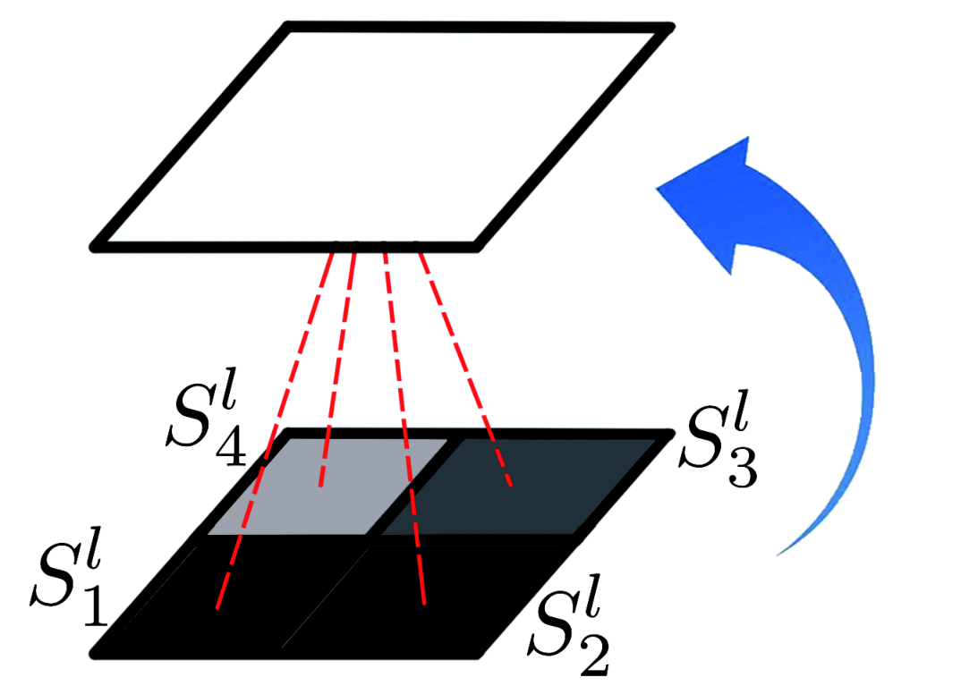
Suppose that we have obtained the clustering result $C^{l}_{1}=\{(C^{l}_{1})_{1}\textrm{,}...\textrm{,}(C^{l}_{1})_{o}\}$ of $S^{l}_{1}$ via FSC, where $o$ ($o\leq k_{1}$) represents the number of the clusters in $C^{l}_{1}$. We use $Q_{1}^{l}$, $Q_{2}^{l}$, $Q_{3}^{l}$, $Q_{4}^{l}$ to represent the indicator matrices of the clustering results of the four child nodes. The entries of matrix $Q_{1}^{l}$ is defined as:

where $|(C^{l}_{1})_{j}|$ is the number of superpixels in cluster $(C^{l}_{1})_{j}$. Similarly, we can define the indicator matrices of the other child nodes in the same way. In particular, suppose that MFSC starts from level $l_{init}$ of the quad-tree. Then each block below level $l_{init}$ is treated as a cluster. Hence its indicator matrix is an identity matrix. With the indicator matrices of the four child nodes, we define matrix

where $s$ is the number of rows in $Q^{l}$ and is equal to the number of superpixels in node $S^{l-1}$; $e$ is the number of the columns of $Q^{l}$ and is equal to the number of the clusters of the four child nodes in total.

Next, cluster set $C^{l}=\displaystyle\bigcup_{i\in\{1\textrm{,}2\textrm{,}3\textrm{,}4\}}C^{l}_{i}$ by FSC. First, the similarity matrix based on superpixel set $C^{l}$ is defined as:

where $W_{S^{l-1}}$ is the similarity matrix based on superpixels of node $S^{l-1}$ and the $s$-order submatrix of $\widetilde{W}$ defined in Eq. (11).

Also, we can define the degree matrix $\widetilde{D}_{S^{l-1}}$ based on the set of superpixels $C^{l}$ of node $S^{l-1}$ as follows:

With matrices $\widetilde{W}_{S^{l-1}}$ and $\widetilde{D}_{S^{l-1}}$, we define the normalized graph Laplacian matrix $\widetilde{L}_{S^{l-1}}$ based on the set of superpixels $C^{l}$ of node $S^{l-1}$ as follows:

Our aim is to further cluster the the set of superpixels $C^{l}$ into $k$ clusters $B=\{B_{1}\textrm{,}B_{2}\textrm{,}\ldots\textrm{,}B_{k}\}$. Analogous to FSC, the clustering result can be obtained by solving the following minimization problem:

where $\widetilde{Q}^{l-1}$ is the indicator matrix of clusters $B$ based on the set of superpixels $C^{l}$.

In order to obtain the indicator matrix based on superpixels $A_{S^{l-1}}$, we convert the indicator matrix $\widetilde{Q}^{l-1}$ to matrix $Q^{l-1}$:

Here, we omit the Fuzzy C-means and treat matrix $Q^{l-1}$ as the indicator matrix of the clustering result of the node $S^{l-1}$.

According to Section III-A, the solution of the problem of Eq. (24) is the first $k$ eigenvectors of matrix $\widetilde{L}_{S^{l-1}}$. It is obvious that the size of matrix $\widetilde{L}_{S^{l-1}}$ is much smaller than that of matrix $\widetilde{L}_{N}$. Therefore, the computational complexity is further reduced.

Repeat the above procedures along the quad-tree structure from the bottom fine level to the top coarse level until the final superpixel-based indicator matrix $Q^{1}$ is obtained. We convert matrix $C_{sup}=\widetilde{D}^{-\frac{1}{2}}Q^{1}$ to $C_{p}$ with the clustering information based on pixels:

where $H$ is defined in Eq. (10). Then we treat each row of $C_{p}$ as a point $\in\mathbb{R}^{k}$ and cluster all of the points into $k$ clusters via the Fuzzy C-means algorithm to obtain the clustering result based on pixels.

The details of MFSC are given in Algorithm 3.

The computational complexity of the proposed FSC consists of the time of quad-tree decomposition, construction of the superpixel-based similarity matrix and eigen-decomposition of the superpixel-based Laplacian matrix. Their computational complexities are $O(n\log n)$, $O(m)$ and $O(m^{\frac{3}{2}})$, respectively, where $n$, $m$ are the number of pixels and that of superpixels respectively. Hence the computational complexity of FSC is $O(n\log n)+O(m)+O(m^{\frac{3}{2}})$. By contrast, Ncut takes $O(n)+O(n^{\frac{3}{2}})$, where $n>m$. The computational complexity of the proposed MFSC consists of the following parts: it takes $O(1)$ to solve the first $k$ eigenvectors of matrix $\widetilde{L}_{S^{l-1}}$, $O(n)$ to compute matrix $\widetilde{L}_{S^{l-1}}$ and $O(n)$ to perform quad-tree decomposition at each level. Hence the method takes $O(n\log{n})$ in total.

The two methods that we propose need to store the superpixel-based similarity matrix $\widetilde{W}$, which counts for the storage of $O(m)$ real-valued numbers since $\widetilde{W}$ is sparse. The memory cost of the two algorithms is much less than that of Ncut $O(n)$.

To show the segmentation results of MFSC and Ncut on single-object images, we select four sample images displayed in Fig.3. $HotAirBalloon$, $Nitpix$ and $Leafpav72$ are selected from Weizmann data set [34], whereas $Tank$ is selected from the database of University of Southern California [35].

1) $HotAirBalloon$. The original size of the image is $300\times 420$. We scale it to $128\times 128$ pixels. We select the following parameters for MFSC: superpixel connection radius $R$ = 40 (Two superpixels are connected in a graph if their center pixels are within distance $R$), threshold of quad-tree decomposition $t=10$, parameters of $\sigma_{I}=8$, $\sigma_{x}=4$, $\sigma_{c}=0.2$ and $\alpha=0.45$ for constructing the similarity matrix. The corresponding parameters of Ncut are set as: pixel connection radius of Ncut $r=20$, $\sigma_{c}=0.1$.

2) $Nitpix$. The original size of the image is $300\times 225$. We scale it to $256\times 256$ pixels. We select the following parameters for MFSC: $R=40$, $t=12$, $\sigma_{I}=8$, $\sigma_{x}=4$, $\sigma_{c}=0.1$, $\alpha=0.45$. The corresponding parameters of Ncut are: $r=15$, $\sigma_{c}=0.1$.

3) $Leafpav72$. The original size of the image is $300\times 203$. We scale it to $512\times 512$ pixels. We select the following parameters for MFSC: $R=80$, $t=12$, $\sigma_{I}=8$, $\sigma_{x}=4$, $\sigma_{c}=0.09$, $\alpha=0.45$. The corresponding parameters of Ncut are: $r=10$, $\sigma_{c}=0.1$.

4) $Tank$. The original size of the image is $512\times 512$. We select the following parameters for MFSC: $R=40$, $t=7$, $\sigma_{I}=0.12$, $\sigma_{x}=0.12$, $\sigma_{c}=0.1$, $\alpha=0.1$. The corresponding parameters of Ncut are: $r=10$, $\sigma_{c}=0.1$.

For multi-object images, we select four sample images displayed in Fig.4. $Plane$, $Imgp1883$, $DualWindows$ and $Yack1$ are all selected from Weizmann data set. We scale them to $256\times 256$.

1)$Plane$. We select the following parameters for MFSC: $R=60$, $t=7$, $\sigma_{I}=8$, $\sigma_{x}=4$, $\sigma_{c}=0.095$, $\alpha=0.45$. The corresponding parameters of Ncut are: $r=15$, $\sigma_{c}=0.1$.

2)$Imgp1883$. We select the following parameters for MFSC: $R=60$, $t=5$, $\sigma_{I}=8$, $\sigma_{x}=4$, $\sigma_{c}=0.095$, $\alpha=0.45$. The corresponding parameters of Ncut are: $r=15$, $\sigma_{c}=0.1$.

3)$DualWindows$. We select the following parameters for MFSC: $R=60$, $t=8$, $\sigma_{I}=8$, $\sigma_{x}=4$, $\sigma_{c}=0.095$, $\alpha=0.45$. The corresponding parameters of Ncut are: $r=15$, $\sigma_{c}=0.1$.

4)$Yack1$. We select the following parameters for MFSC: $R=60$, $t=8$, $\sigma_{I}=8$, $\sigma_{x}=4$, $\sigma_{c}=0.095$, $\alpha=0.45$. The corresponding parameters of Ncut are: $r=15$, $\sigma_{c}=0.1$.

We evaluate the segmentation quality by Accuracy (ACC) [36], Rand index (RI) [38] and Dice coefficient (Dice) [37]. Given pixel $v_{i}$, let $o_{i}$, $s_{i}$, $F$, $B$ be its resultant segmentation label, ground-truth label, foreground and background, respectively.

$\bm{ACC}$: Define

where $\delta(a\textrm{,}b)$ denotes the delta function that returns $1$ if $a=b$ and $0$ otherwise; $map(v_{i}\textrm{,}o_{i})$ is the best mapping function for permuting the cluster labels to match the ground-truth labels. The larger the ACC is, the better the segmentation performance is.

$\bm{RI}$: Define

where

where $m_{ij}=|o_{i}\bigcap s_{j}|\$, $i\textrm{,}j\in\{F\textrm{,}B\}$. The range of RI is in the interval of 0 and 1, where 0 is for absolute mismatch and 1 for equality to the ground truth.

$\bm{Dice}$: Define

Its range is from 0 to 1 (1 for perfect match with ground truth).

All of our experiments are conducted on a Windows 10 x64 computer with a 3.4 GHz Intel(R) Core(TM) i7-3770 CPU and 8 GB RAM, MATLAB.

We study the relationship between the threshold of quad-tree decomposition and the performance of MFSC. We take an image from Weizmann data set as an example. Fig.7 shows the segmentation result of the image under different thresholds of quad-tree decomposition with MFSC. It can be observed that the larger the threshold is, the worse the result is, the shorter the computing time is. The relationship is presented more clearly via the parameters of computing time and RI in Fig.8. However, it can also be observed that the segmentation performance is robust to the threshold when the threshold is smaller than a certain value. The reason behind is that under this circumstances, the quad-tree structure can show the complete texture/shape cues when the threshold is below some value. We empirically set the threshold for $128\times 128$ images to be $10$, $256\times 256$ $12$, $512\times 512$ $16$, which is appropriate to most images used in our experiments.

References

- [1] Langone, Rocco, and Johan AK Suykens. “Fast kernel spectral clustering.¡± Neurocomputing, vol. 268, pp. 27-33, 2017.
- [2] Zhang, Hui, Q. M. J. Wu, and T. M. Nguyen. “Image segmentation by a robust generalized fuzzy c-means algorithm.” IEEE International Conference on Image Processing IEEE, pp. 4024-4028, 2014.
- [3] Zhou, Zhili, et al. “Fast and accurate near-duplicate image elimination for visual sensor networks.” International Journal of Distributed Sensor Networks, vol. 13, no. 2, pp. 1550147717694172, 2017.
- [4] Yu, Zhiwen, et al. “Adaptive fuzzy consensus clustering framework for clustering analysis of cancer data.” IEEE/ACM Transactions on Computational Biology and Bioinformatics (TCBB), vol. 12, no. 4, pp. 887-901, 2015.
- [5] Rong, Huan, et al. “A novel subgraph -isomorphism method in social network based on graph similarity detection.” Soft Computing, vol. 22, no. 8, pp. 2583-2601, 2018.
- [6] Balla-Arab¨¦, Souleymane, Xinbo Gao, and Bin Wang. “A fast and robust level set method for image segmentation using fuzzy clustering and lattice Boltzmann method.” IEEE transactions on cybernetics, vol. 43, no. 3, pp. 910-920, 2013.
- [7] Li, Ping, et al. “Relational multimanifold coclustering.” IEEE Transactions on cybernetics, vol. 43, no. 6, pp. 1871-1881, 2013.
- [8] Liu, Yanchi, et al. “Understanding and enhancement of internal clustering validation measures.” IEEE transactions on cybernetics, vol. 43, no. 3, pp. 982-994, 2013.
- [9] Hartigan, John A., and Manchek A. Wong. “Algorithm AS 136: A k-means clustering algorithm.” Journal of the Royal Statistical Society. Series C (Applied Statistics), vol. 28, no. 1, pp. 100-108, 1979.
- [10] Zhan, Qiang, and Yu Mao. “Improved spectral clustering based on Nystrm method.” Multimedia Tools and Applications, vol. 76, no. 19, pp. 20149-20165, 2017.
- [11] Filippone, Maurizio, et al. “A survey of kernel and spectral methods for clustering.” Pattern recognition, vol. 41, no. 1, pp. 176-190, 2008.
- [12] Wang, Rong, Feiping Nie, and Weizhong Yu. “Fast Spectral Clustering With Anchor Graph for Large Hyperspectral Images.” IEEE Geoscience and Remote Sensing Letters, vol. 14, no. 11, pp. 2003-2007, 2017.
- [13] Tung, Frederick, A. Wong, and D. A. Clausi. “Enabling scalable spectral clustering for image segmentation.” Pattern Recognition, vol. 43, no. 12, pp. 4069-4076, 2010.
- [14] He, L., et al. “Fast Large-Scale Spectral Clustering via Explicit Feature Mapping.” IEEE Transactions on Cybernetics, 2018.
- [15] Semertzidis, T., et al. “Large-scale spectral clustering based on pairwise constraints.” Information Processing Management, vol. 51, no. 5, pp. 616-624, 2015.
- [16] Cao, Jiangzhong, et al. “Local information-based fast approximate spectral clustering.” Pattern Recognition Letters, vol. 38, no. 1, pp. 63-69, 2014.
- [17] Hagen, Lars, and Andrew B. Kahng. “New spectral methods for ratio cut partitioning and clustering.” IEEE transactions on computer-aided design ofintegrated circuits and systems, vol. 11, no. 9, pp. 1074-1085, Sep 1992.
- [18] Jianbo Shi and J. Malik, “Normalized cuts and image segmentation,” in IEEE Transactions on Pattern Analysis and Machine Intelligence, vol. 22, no. 8, pp. 888-905, Aug 2000.
- [19] T. Cour, F. Benezit and J. Shi, “Spectral segmentation with multiscale graph decomposition,” 2005 IEEE Computer Society Conference on Computer Vision and Pattern Recognition (CVPR’05), vol. 2, pp. 1124-1131, 2005.
- [20] C. Fowlkes, S. Belongie, F. Chung and J. Malik, “Spectral grouping using the Nystrom method,” in IEEE Transactions on Pattern Analysis and Machine Intelligence, vol. 26, no. 2, pp. 214-225, Feb. 2004.
- [21] Yan, Donghui, Ling Huang, and Michael I. Jordan. “Fast approximate spectral clustering.” Proceedings of the 15th ACM SIGKDD international conference on Knowledge discovery and data mining. ACM, pp. 907-916, 2009.
- [22] Cai, Deng, and Xinlei Chen. “Large scale spectral clustering via landmark-based sparse representation.” IEEE transactions on cybernetics, vol. 45, no. 8, pp. 1669-1680, 2015.
- [23] Jain, Anil K., M. Narasimha Murty, and Patrick J. Flynn. “Data clustering: a review.” ACM computing surveys (CSUR), vol. 31, no. 3, pp. 264-323, 1999.
- [24] Von Luxburg, Ulrike. “A tutorial on spectral clustering.” Statistics and computing, vol. 17, no. 4, pp. 395-416, 2007.
- [25] Ng, Andrew Y., Michael I. Jordan, and Yair Weiss. “On spectral clustering: Analysis and an algorithm.” Advances in neural information processing systems, pp. 849-856, 2002.
- [26] Lutkepohl, Helmut.“Handbook of matrices.” Computational statistics and Data analysis, 2.25, pp. 243, 1997.
- [27] Nascimento, Maria C. V , and de Carvalho, Andre C. P. L. F. “Spectral methods for graph clustering ¨C A survey.” European Journal of Operational Research, vol. 211, no. 2, pp. 221-231, 2011.
- [28] Spann, Michael, and Roland Wilson. “A quad-tree approach to image segmentation which combines statistical and spatial information.” Pattern Recognition, vol. 18, no. 3-4, pp. 257-269, 1985.
- [29] Elsayed, Ashraf, et al. “Corpus callosum MR image classification.” Research and Development in Intelligent Systems XXVI. Springer, London, pp. 333-346, 2010.
- [30] Allen, Laura S., et al. “Sex differences in the corpus callosum of the living human being.” Journal of Neuroscience, vol. 11, no. 4, pp. 933-942, 1991.
- [31] Davatzikos, Christos, et al. “A computerized approach for morphological analysis of the corpus callosum.” Journal of computer assisted tomography, vol. 20, no. 1, pp. 88-97, 1996.
- [32] Weis, Serge, et al. “Morphometric analysis of the corpus callosum using MR: correlation of measurements with aging in healthy individuals.” American Journal of Neuroradiology, vol. 14, no. 3, pp. 637-645, 1993.
- [33] Bezdek, James C., Robert Ehrlich, and William Full. “FCM: The fuzzy c-means clustering algorithm.” Computers & Geosciences, vol 10, no. 2-3, pp. 191-203, 1984.
- [34] http://www.wisdom.weizmann.ac.il/~vision/Seg_Evaluation_DB/
- [35] http://sipi.usc.edu/database/database.php?volume=misc
- [36] Jia, Yuheng, Sam Kwong, and Junhui Hou. “Semi-Supervised Spectral Clustering With Structured Sparsity Regularization.” IEEE Signal Processing Letters, vol. 25, no. 3, pp. 403-407, 2018.
- [37] Dice, Lee R. “Measures of the amount of ecologic association between species.” Ecology, vol. 26, no. 3, pp. 297-302, 1945.
- [38] Rand, William M. “Objective criteria for the evaluation of clustering methods.” Journal of the American Statistical association, vol. 66, no. 336, pp. 846-850, 1971.
![[Uncaptioned image]](1812.04816v1/zhang.png) |
Chongyang Zhang is currently pursuing the M.Eng. degree in the School of Electronic and Information Engineering from Soochow Univerity. His research interests is machine learning and image processing. |
![[Uncaptioned image]](1812.04816v1/zhu.png) |
Guofeng Zhu is currently pursuing the M.S. degree in the School of Mathematical Sciences from Soochow Univerity. His research interests is machine learning and image processing. |
![[Uncaptioned image]](1812.04816v1/cmx.png) |
Minxin Chen Minxin Chen is Associated Professor of computational mathematics at Soochow University, Suzhou, China. He received his Ph.D. in Computational mathematics at Chinese Academy of Sciences, Beijing, China. His research interests are in, image processing, and computational mathematics. |
![[Uncaptioned image]](1812.04816v1/ch.png) |
Hong Chen Hong Chen was born in Suzhou, Jiangsu Province, China, in 1983. She received her B.S.degree in School of Mathematical Sciences from Soochow University, Suzhou, China, in 2006, and she received her Ph.D degree in fundamental mathematics from Graduate University of Chinese Academy of Sciences, Beijing, China, in 2011. From 2011 until now, she worked in School of Mathematical Sciences from Soochow University. She is currently working mainly on image processing and Mathematical modeling. |
![[Uncaptioned image]](1812.04816v1/wcj.png) |
Chenjian Wu Chenjian Wu was born in Suzhou, Jiangsu Province, China, in 1983.Chenjian Wu received his B.S. degree in Information Engineering from Southeast University, Nanjing, China, in 2006, and he received his M.S. degree in Software Engineering from Southeast University in 2010 and Ph.D degree in Electronic Circuit and System from Southeast University in 2013. From August 2013 until now, he worked in School of Electronic and Information Engineering, Soochow University, Suzhou, Jiangsu. He is currently working mainly on image processing and artificial intelligence chip design. |