Regression-Based Bayesian Estimation and Structure Learning for Nonparanormal Graphical ModelsPublication type: Article Type
Abstract
A nonparanormal graphical model is a semiparametric generalization of a Gaussian graphical model for continuous variables in which it is assumed that the variables follow a Gaussian graphical model only after some unknown smooth monotone transformations. We consider a Bayesian approach to inference in a nonparanormal graphical model in which we put priors on the unknown transformations through a random series based on B-splines. We use a regression formulation to construct the likelihood through the Cholesky decomposition on the underlying precision matrix of the transformed variables and put shrinkage priors on the regression coefficients. We apply a plug-in variational Bayesian algorithm for learning the sparse precision matrix and compare the performance to a posterior Gibbs sampling scheme in a simulation study. We finally apply the proposed methods to a real data set.
keywords
Bayesian inference, Cholesky decomposition, nonparanormal graphical models, continuous shrinkage priorMulgrave, J. J. et al
1 Introduction
The Gaussian graphical model (GGM) is a mathematical model commonly used to describe conditional independence relationships among normally distributed random variables. The estimation of the underlying graph in a GGM is known as structure learning. Zeros in the inverse covariance matrix, or the precision matrix, indicate that the corresponding variables in the data set are conditionally independent given the rest of the variables in the data set, and this relationship is represented by the absence of an edge in the graph. Similarly, nonzero entries in the precision matrix are represented by edges in the graph and correspond to conditionally dependent variables in the data set. Thus, an assumed sparsity condition is used to learn the conditional dependence structure in a GGM. An extension of the GGM is the nonparanormal graphical model (Liu et al. 2009) in which the random variables are replaced by transformed variables that are assumed to be normally distributed. Liu et al. 2009 use a truncated empirical distribution function to estimate the functions and then estimate the precision matrix of the transformed variables using the graphical lasso. The Bayesian method for the nonparanormal graphical model (Mulgrave and Ghosal 2020) uses a random series B-splines prior to estimate the functions and a Student-t spike-and-slab prior to estimate the resulting precision matrix. These extensions differ from the Gaussian copula graphical model (Pitt et al. 2006; Dobra and Lenkoski 2011; Liu et al. 2012; Mohammadi et al. 2017) in that the nonparanormal graphical model concurrently estimates the transformation functions and the precision matrices. Nonparanormal graphical model approaches have been applied to discrete data models of interactions between genes Nguyen and Chiogna 2018 and to test differential gene networks Zhang 2020.
Estimation of a sparse precision matrix is necessary to learn the structure in GGMs and nonparanormal graphical models. For unstructured precision matrices, a commonly used algorithm in the frequentist literature is the graphical lasso (Friedman et al. 2008). A great number of algorithms have been proposed to solve this problem including Meinshausen and Buhlmann 2006; Yuan and Lin 2007; Friedman et al. 2008; Banerjee et al. 2008; d’Aspremont et al. 2008; Rothman et al. 2008; Lu 2009; Scheinberg et al. 2010; Witten et al. 2011; Mazumder and Hastie 2012b.
Analogous methods in the Bayesian literature use priors to aid the edge selection procedure. For instance, off-diagonal entries of the precision matrix may be set to zero by allowing a point mass at zero in the prior (Banerjee and Ghosal 2015), but the posterior is harder to compute or sample from. A normal spike-and-slab prior (Wang 2015) replaces the point mass at zero by a highly concentrated normal distribution around zero and similarly, a Laplace spike-and-slab prior (Gan et al. 2019) has been used. From a computational point of view, continuous shrinkage priors such as the horseshoe prior (Carvalho et al. 2009), the Dirichlet-Laplace prior (Bhattacharya et al. 2015), and generalized double exponential prior (Armagan et al. 2013), bring in the effects of both a point mass and a thick tail by a single continuous distribution with an infinite spike at zero.
Ideally, we seek solutions that guarantee a sparse positive definite matrix using continuous shrinkage priors. Since continuous shrinkage priors do not assign exact zeros, a variable selection procedure needs to be used to determine which of the small and nonzero elements should be specified as exactly zero. Methods that use spike and slab priors naturally incorporate variable selection, whereas methods that use alternative priors need a thresholding procedure. However, post-hoc thresholding procedures do not guarantee a positive definite precision matrix. The methods in Wang 2015 and Wang 2012 guarantee a positive definite matrix by way of the sampling algorithm. Wang 2012 and Peterson et al. 2013 use the double exponential prior and improve on its use for sparsity by allowing each double exponential prior to have its own shrinkage parameter. More recent methods estimate the inverse covariance matrix by using the normal spike and slab prior (Wang 2015; Peterson et al. 2016; Li et al. 2019; Li and McCormick 2019) for variable selection in the graphical model context. Lastly, (Williams et al. 2018) constructs Gaussian graphical models by estimating the partial correlation matrix using a horseshoe prior for regularization and for sparsity, using projection predictive selection, a method that allows for variable exclusion based on predictive utility, with good results.
Utilizing a Cholesky decomposition is an alternative way to incorporate the positive definiteness constraint on precision matrices, but is very dependent on the ordering of the variables (Pourahmadi 2011). We consider a prior based on Cholesky decomposition of the precision matrix that reduces this dependence. We derive a sparsity constraint that ensures a weak order invariance in that it maintains the same order of sparsity in the rows of the precision matrix by increasing the order of sparsity down the rows of the lower triangular matrix. We construct a pseudo-likelihood through regression of each variable on the preceding ones. The approach splits the very high dimensional original problem to several lower dimensional ones. The method in Wong et al. 2013 is also based on Cholesky decomposition, but it uses a noninformative Jeffreys’ prior and the ordering issue of the Cholesky decomposition is not addressed.
We consider two different priors, the horseshoe and the Bernoulli-Gaussian (Soussen et al. 2011). These priors have clear interpretations of the probability of nonzero elements (Soussen et al. 2011; van der Pas et al. 2014), which allows us to effectively calibrate sparsity. The strength of the Bernoulli-Gaussian prior is that it leads to a sparse positive definite precision matrix that does not require thresholding and the strength of the horseshoe prior is that it is a better model of sparsity than the Bernoulli-Gaussian prior due to its heavier tails. Horseshoe priors have not yet been used for Bayesian nonparanormal graphical models that use transformation functions. We compare the performance of the methods using both a variational Bayesian algorithm and a full Markov chain Monte Carlo (MCMC) sampling scheme. Mean field variational Bayes (Jordan et al. 1999; Wainwright and Jordan 2007) is an alternative to MCMC that allows for faster fitting by deterministic optimization. A variational Bayesian method for Gaussian graphical models is developed in Chen et al. 2011 and an expectation conditional-maximization approach is used by Li and McCormick 2019 in Gaussian copula graphical models. This approach has not yet been explored in the setting of a nonparanormal graphical model. We wish to determine if we can retain the information learned in a Bayesian nonparanormal graphical model while speeding up the estimation process using variational Bayesian techniques.
The paper is organized as follows. In the next section, we describe the model and the sparsity constraint. In Section 3, we describe the variational Bayesian algorithm. In Sections 4 and 5, we discuss particular priors and their corresponding Markov Chain Monte Carlo algorithms. In Section 6, we describe a thresholding procedure and in Section 7, we detail the tuning procedure. In Section 8, we present a simulation study. In Section 9, we describe a real data application.
2 Model and Priors
2.1 Nonparanormal Transformation
Definition 2.1.
A random vector has a nonparanormal distribution if there exist smooth monotone functions such that , a normal distribution with mean , covariance matrix , and dimension , and where . In this case we shall write .
We put prior distributions on the unknown transformation functions through a random series based on B-splines. In Mulgrave and Ghosal 2020, we have described the prior distributions, including the motivation and support for the choices made, in greater detail. We briefly describe the prior in this section. We represent the transformation functions in a nonparanormal model through a basis expansion
| (1) |
where each are coefficients, are the B-spline basis functions, , , and is the number of B-spline basis functions used in the expansion. We assume that the precision matrix is sparse, in that, most of its off-diagonal entries are zero. However, the model is not identifiable, since location-scale changes in the transformation functions and the normal distributions can be cancelled by each other. To resolve the issue, one possibility is to fix the mean-vector to zero and assume that the covariance matrix is a correlation matrix, but putting a prior on such a matrix maintaining sparsity of its inverse appears inconvenient. Therefore, we let the mean and the precision matrix be free parameters while putting restrictions on the transformations. We begin with a normal prior on each of the coefficients of the B-splines, , that is set to be , where is some positive constant, is some vector of constants, and is the identity matrix, and impose a monotonicity restriction on them to make the transformation monotone (see below for details). We impose the following two linear constraints on the coefficients through function values of the transformations: and The linear constraints can be written in matrix/vector form as for each . The linear nature of the constraints allow us to retain the joint normality of the coefficient vectors before the monotonicity restriction, and hence a truncated joint normal after the restriction is imposed.
By the properties of a B-spline basis function, if the B-spline coefficients, are increasing in , then is an increasing function. We thus impose the monotonicity constraint on the coefficients, which is equivalent with the series of inequalities . The monotonicity constraint can be expressed in matrix/vector form as for each . Thus, the prior on the coefficients before the truncation is imposed is given by where the prior mean and variance are and . To ensure we have a Lebesgue density on , we work with a dimension-reduced coefficient vector by removing two coefficients and we denote this reduction with a bar over the vector and matrix.
The final prior on the coefficients is given by a truncated normal prior distribution where is the dimension-reduced coefficient vector with the dimension-reduced mean vector , dimension-reduced covariance matrix , restriction . Additionally, is the dimension-reduced matrix of the monotonicity constraints and is a dimension-reduced constant vector of the monotonocity constraints. We denote the truncated normal distribution as with mean , covariance matrix , restriction , and dimension . Any choice of is acceptable, but we use , where is a constant, is a positive constant, and is the inverse of the cumulative distribution function of the standard normal distribution. The idea is that by increasing the original components of the mean vector , the truncation set in the final prior of the B-spline coefficients will have a substantial prior probability.
Finally, we put an improper uniform prior on the mean . The resulting transformed variables, , which are assumed to be distributed as and , , are used to estimate the precision matrix and learn the structure of the underlying graph.
2.2 Cholesky Decomposition Reformulated as Regression Problems
We learn the structure of the precision matrix using a Cholesky decomposition. Denote the Cholesky decomposition of as , where is a lower triangular matrix with elements . Define the coefficients and the precision as . Then as described in (Wong et al. 2013), the lower triangular entries of , denoted as , are given by
Accordingly, the multivariate Gaussian model is equivalent to the set of independent regression problems,
where are the regression coefficients for and , and and are, respectively, the th column and th columns selected from matrix . We use the notation to indicate that the columns are greater than the th column.
We use a standard conjugate noninformative prior on the variances. We consider two different continuous shrinkage priors on the regression coefficients, the horseshoe prior and the Bernoulli-Gaussian prior. Using these priors, we enforce a sparsity constraint along the rows of the lower triangular matrix. The sparsity constraint is one in which the global sparsity parameter of the continuous shrinkage prior is scaled by , where and . Using this constraint, we expect that the precision matrix will be sparse through weak order invariance. The sparsity constraint is derived in the next subsection.
2.3 Sparsity Constraint
In order to ensure that the probability that an entry is nonzero (i.e. sparsity) remains roughly the same over different rows we cannot simply impose the same degree of sparsity on the rows of the Cholesky factor , but need to change it over rows appropriately. Denote the probability as . To see how the Cholesky factor depends on the row index, we observe that
Let P(Nonzero entry in the th row of ). Then
If , the expression is roughly , which remains stable in if , where depends on but not on . Then we obtain the probability of non-zero to be . Further, choosing to be small for makes the probability small, which is essential in higher dimension. We choose P(nonzero in th row), and tune the value of to cover a range of three orders of magnitude, i.e. .
3 Variational Bayes Estimation
We observe independent samples, , from the nonparanormal model with a sparse . Based on these observations and the prior described in Section 2.1, we intend to compute the posterior distribution to make inferences about and its structure, using the transformations . Ideally, we would want to construct a complete variational Bayesian (VB) algorithm in which the B-spline coefficients, mean, and inverse covariance matrix are estimated all in one setting. However, for our problem, there is no closed form solution for the truncated multivariate normal distribution, and closed form solutions are needed for the mean field variational Bayesian algorithms. Instead, we use an exact Hamiltonian Monte Carlo within Gibbs scheme to sample the B-spline coefficients and the mean. We obtain the Bayes estimate of the B-spline coefficients, , and the Bayes estimate of the mean, , where is the posterior mean operator. We then apply the variational Bayesian method on the synthetic data obtained by transforming the original observations using the estimated transformations. Thus we estimate the transformed variables using
Ideally, instead of plugging in, one can obtain samples from the posterior distributions of the transformations and draw samples from the variational distributions of the precision matrix for each generated sample and accumulate them. However, even in moderately high dimension, such an approach is extremely computationally intensive. Since the posterior distributions of the transformations are consistent (Mulgrave and Ghosal 2020), they concentrate near the Bayes estimate. As the main goal is structure learning, the inability of the plug-in to assess the posterior variability of the transformations is not a highly deterring issue. Thus, although the proposed algorithm is not fully Bayesian, it utilizes the strength of the variational Bayesian approach to identify conditional independence relations in a nonparanormal graphical model within a manageable time. While the variational inference generally underestimates the posterior variance Blei et al. 2017, since the goal of structure learning is to determine whether there are zeros or nonzeros in the precision matrix, we should still be able to determine whether the element is zero or not zero. We illustrate the variational method on the Bernoulli-Gaussian prior, following the strategy described in Ormerod et al. 2017. Let the Bernoulli distribution be denoted as and the inverse gamma distribution be denoted as with shape parameter and scale parameter . We can describe the joint distribution by
| (2) | ||||
for , where is the vector of regression coefficients, is the matrix of transformations, and is a binary indicator matrix of 0s and 1s that is modeled by the Bernoulli distribution with elements . The hyperparameters , and , are fixed, and controls the sparsity. This variant of the spike-and-slab prior indirectly models sparsity on the regression coefficients by putting a binary indicator on the regression coefficients in the likelihood, instead of directly modeling sparsity on the regression coefficients. As such, if for the Bernoulli-Gaussian prior, then , unlike in usual spike-and-slab priors in which would be equal to exactly 0. We select using a tuning procedure that incorporates the sparsity constraint and is discussed in Subsection 3.1.
The joint posterior distribution that we aim to compute is
By plugging in the estimated transformed variables, we use a variational Bayesian algorithm to compute the posterior distribution of the sparse precision matrix. Mean field variational Bayesian inference involves minimizing the Kullback-Leibler divergence between the true posterior distribution and a factorized approximation of the posterior. Let represent the set of parameters in the model and represent the matrix of estimated transformed variables. Then is approximated by , where is a partition of . The optimal densities satisfy
where is the expectation with respect to all densities except (Bishop 2006). The variational lower bound (VLB) for the marginal likelihood for is then given by
where is the expectation with respect to the density . Using the coordinate ascent method, optimizing each while holding the others fixed will result in the algorithm converging to a local maximum of the lower bound.
Following (Ormerod et al. 2017), the choice of factorization that we use for the VB approximation is
with, for some choice of parameters,
The parameters are obtained by the VLB with respect to them by coordinate ascents, called variational updates, which we can derive as in Ormerod et al. 2017. Introduce the notations , and , and let the symbol denote the Hadamard product between two matrices. Then we have
for , and . Note that we use the notation to indicate that the columns are greater than the th column. In addition, where , , and .
Using these optimal densities, the VLB simplifies to
| (3) |
The variational Bayesian algorithm is detailed in the Appendix.
3.1 Tuning Procedure
For every regression problem, we choose the parameter based on the tuning algorithm described in detail in Section 4 of Ormerod et al. 2017. In this section, we describe the changes that we made to add the sparsity constraint. We use the discussed in Ormerod et al. 2017 and multiply that value with to incorporate the sparsity constraint discussed in Section 2.3. Thus, for the fixed that was discussed in Ormerod et al. 2017, for our work, that translates to . Note that since the dimension is not changing for , we do not need to include for tuning. For the fixed that was discussed in Ormerod et al. 2017, for our work, that translates to the fixed , and we select , where is taken from an equally spaced grid of 50 points between 0.1 and 10, and varies over an equally spaced grid of 50 points between and . We replace the with which leads a grid of 50 values of between and instead of the three values of that was discussed in Section 2.3. The variational lower bound for the tuning procedure is only based on the preceding regressions and not the regression relations that involve and .
4 MCMC Estimation through Horseshoe Prior
4.1 Horseshoe Prior
We use the horseshoe prior described in Neville et al. 2014, to shrink the coefficients:
| (4) | ||||
for , where , is the matrix of transformations, and and are fixed hyperparameters.
The global scale parameter is roughly equivalent to the probability of a nonzero element (van der Pas et al. 2014). We enforce the sparsity constraint using, . Thus, since we are working with the squared parameter, the factor in the variance term for is , where .
The joint posterior distribution, corresponding conditional posterior distributions, and the sampling algorithm are provided in the Appendix.
5 MCMC Estimation through Bernoulli-Gaussian Prior
5.1 Bernoulli-Gaussian Prior
We use the same Bernoulli-Gaussian prior described in (2). The joint posterior distribution, corresponding conditional posterior distributions, and the sampling algorithm are provided in the Appendix.
6 Thresholding
The thresholding procedure that we consider for the method using the horseshoe prior (4) is based on a 0-1 loss function described in (Wang 2012) for classification under absolutely continuous priors. Although this procedure is heuristic, it seems to perform well in practice. Other thresholding rules may be used, such as those based on posterior credible intervals (Khondker et al. 2013), information criterion (Kuismin and Sillanpää 2016), clustering (Li and Pati 2017), posterior model probabilities (Banerjee and Ghosal 2015; Mohammadi and Wit 2015), and projection predictive selection (Williams et al. 2018), but we chose to focus on the 0-1 loss procedure for this study.
6.1 0-1 Loss Procedure
We find the posterior partial correlation using the precision matrices from the Gibbs sampler of the horseshoe prior (4) and the posterior partial correlation using the standard conjugate Wishart prior. The posterior samples of the partial correlation using the precision matrices from the Gibbs sampler are defined as
where is a Markov chain Monte Carlo (MCMC) sample from the posterior distribution of , where , is the number of MCMC samples, and . The posterior partial correlation using the standard conjugate Wishart prior is found by starting with the latent observation, which is obtained from the MCMC output. We put a standard Wishart prior on the precision matrix, Wang 2012, where is the identity matrix. Note that this Wishart prior does not assume sparsity, but is obtained from the MCMC output assuming sparsity of the precision matrix. Through conjugacy, the posterior distribution is , where . We then calculate the mean of the posterior distribution, . Finally, we compute the posterior samples of partial correlation coefficients by conjugate Wishart prior as
where stands for the th element of .
We link these two posterior partial correlations for the 0-1 loss method. We claim the event if and only if
| (5) |
for and . The idea is that we are comparing the regularized precision matrix from the horseshoe prior to the non-regularized precision matrix from the Wishart prior. If the absolute value of the partial correlation coefficient from the regularized precision matrix is similar in size or larger than the absolute value of the partial correlation coefficient from the Wishart precision matrix, then there should be an edge in the edge matrix. If the absolute value of the partial correlation coefficient from the regularized precision matrix is much smaller than the absolute value of the coefficient from the Wishart matrix, then there should not be an edge in the edge matrix.
7 Choice of Prior Parameters
For the precision matrix being estimated with a horseshoe prior (4), we need to select the value of the parameter which controls the sparsity. We solve a convex constrained optimization problem in order to use the Bayesian Information Criterion (BIC), as described in Dahl et al. 2005; Dahl et al. 2008. First, we find the Bayes estimate of the inverse covariance matrix, . We also find the average of the transformed variables, , where , , are obtained from the MCMC output. Then, using the sum of squares matrix , we solve for , the maximum likelihood estimate of the inverse covariance matrix,
where represents the constraint that all elements of at the locations of the zeros of the estimated edge matrix from the MCMC sampler are zero. The estimated edge matrix from the MCMC sampler will be described in more detail in Section 8. For computational simplicity, in the code, we represent this problem as an unconstrained optimization problem as described in Dahl et al. 2005; Dahl et al. 2008.
Lastly, we calculate , where , the sum of the number of diagonal elements and the number of edges in the estimated edge matrix, and . We select the that results in the smallest BIC.
8 Simulation Results
We conduct a simulation study to assess the performance of the proposed methods using the horseshoe MCMC, indicated as Horseshoe, Bernoulli-Gaussian MCMC, indicated as Bernoulli-Gaussian, and variational Bayesian algorithm, indicated as Variational Bayes. We choose not to include to the Bayesian nonparanormal graphical model described in Mulgrave and Ghosal 2020 because we want to maintain the Cholesky decomposition across all comparisons of the proposed methods. We compare the structure learning results of our methods to the nonparanormal graphical model (Liu et al. 2009) and to a Bayesian Gaussian copula graphical model (Mohammadi et al. 2017), indicated as the Bayesian Copula, in which the rank likelihood is used to transform the random variables with a uniform prior on the graph, a G-Wishart prior on the inverse correlation matrix, and estimation is used with the birth-death MCMC (Mohammadi and Wit 2015). These competing methods all utilize a transformation of the data to learn the graphical structure.
We assess the performance of these methods by calculating sensitivity, specificity, and the Matthews correlation coefficient (MCC). We assess the effect of the transformation functions of our proposed methods by calculating the scaled -loss. These metrics are detailed in Subsection 8.1. In this section, we describe the data generation process used to conduct the simulation study.
The random variables, , are simulated from a multivariate normal distribution such that for . The means are selected from an equally spaced grid between 0 and 2 with length . We consider nine different combinations of and sparsity for :
- •
, , sparsity = non-zero entries in the off-diagonals;
- •
, , sparsity = non-zero entries in the off-diagonals;
- •
, , sparsity = non-zero entries in the off-diagonals;
- •
, AR(2) model;
- •
, , AR(2) model;
- •
, , AR(2) model;
- •
, circle model;
- •
, , circle model;
- •
, , circle model,
where the circle model and the AR(2) model are described by the relations
- •
Circle model: , and ;
- •
AR(2) model: and .
The percent sparsity levels for are computed using lower triangular matrices that have diagonal entries normally distributed with and , and non-zero off-diagonal entries normally distributed with and , where denotes the complement of the set.
The observed variables are constructed from the simulated variables . The functions used to construct the observed variables are three cumulative distribution functions (c.d.f.s): asymmetric Laplace, extreme value, and stable. Any values of the parameters for the c.d.f.s could be chosen, but instead of selecting 25, 50, and 100 sets of parameters, we automatically choose the values of the parameters to be the maximum likelihood estimates with the mle function in MATLAB. The values of the parameters for each of the c.d.f.s are the maximum likelihood estimates for the parameters of the corresponding distributions (asymmetric Laplace, extreme value, and stable), using the variables .
We follow the procedure in Mulgrave and Ghosal 2020 to estimate the transformation functions. The hyperparameters for the normal prior are chosen to be and . To choose the number of basis functions, we use the Akaike Information Criterion as described in Mulgrave and Ghosal 2020. Samples from the truncated multivariate normal posterior distributions for the B-spline coefficients are obtained using the exact Hamiltonian Monte Carlo (exact HMC) algorithm (Pakman and Paninski 2014). The initial coefficient values, , for the exact HMC algorithm are calculated using quadratic programming as described in (Mulgrave and Ghosal 2020). After finding the initial coefficient values , we construct initial values for using the observed variables. These initial values are used to find the initial values for , and for the algorithm, where , where is the average of , and .
For the part of the simulation study in which we do not estimate the transformation functions, the initial values for the Horseshoe, Bernoulli-Gaussian, and Variational Bayes algorithms are constructed from the observed variables, , with , where is the average of , and . Afterwards, the mean and the precision matrix are estimated using the algorithms as described in the previous sections.
The hyperparameter for the Bernoulli-Gaussian prior and the Variational Bayes algorithm is fixed at 10. The hyperparameters and for the inverse gamma distribution for the Bernoulli-Gaussian prior, the Variational Bayes algorithm, and the horseshoe prior, are fixed at . The initial value, , where , for the Variational Bayes algorithm is chosen to be 1000. The threshold for stopping the Variational Bayes algorithm is set to . For the Variational Bayes algorithm and the MCMC algorithm using the Bernoulli-Gaussian prior, the tuning procedure described in Subsection 3.1 is used to find the hyperparameter for the Bernoulli distribution, . Since the vector from the tuning procedure consists of only 0 and 1 values, it is used as the initial indicator vector for the MCMC algorithm using the Bernoulli-Gaussian prior. The data matrix that is used as input for the tuning procedure is , which was described in the previous paragraphs.
For the MCMC algorithm for the horseshoe prior, we consider three values of that are a range of three orders of magnitude: . The value of that yields the lowest BIC was selected for the final estimates of the precision matrix and edge matrix. The 0-1 loss procedure described in Subsection 6.1 was used to threshold the precision matrices and construct the edge matrices.
For the simulation study, we run 100 replications for each of the nine combinations and assess structure learning for each replication. We collect MCMC samples for inference after discarding a burn-in of . We do not apply thinning. The Bayesian copula method is implemented using the R package, BDGraph (Mohammadi and Wit 2019) using the option “gcgm”. Posterior graph selection is done using Bayesian model averaging, the default option in the BDGraph package, in which it selects the graph with links for which their estimated posterior probabilities are greater than 0.5. The nonparanormal graphical model is implemented using the R package huge (Zhao et al. 2015) using the option “truncation”. The graphical lasso method is selected for the graph estimation and the default screening method, lossless (Witten et al. 2011; Mazumder and Hastie 2012a), is used. Three regularization selection methods are used to find the estimated precision matrix and select the graphical model: the Stability Approach for Regularization Selection (StARS) (Liu et al. 2010), the modified Rotation Information Criterion (RIC) (Lysen 2009), and the Extended Bayesian Information Criterion (EBIC) (Foygel and Drton 2010). The default parameters in the huge package are used for each selection method. As in Liu et al. 2009, the number of regularization parameters used is 50 and they are selected among an evenly spaced grid in the interval [0.16, 1.2].
The code for the proposed Bayesian methods is written in MATLAB and sparse representations of the matrices are used when appropriate. For the Variational Bayes algorithm, when calculating , it is set to 0 if is below , which is eps, the floating-point relative accuracy in MATLAB, while is set to 1 if is equal to infinity in MATLAB for numerical stability. Infinity results from operations that lead to results too large to represent as conventional floating-point values. Similar adjustments are also applied for the Bernoulli-Gaussian MCMC. The code is given in the Appendix.
8.1 Performance Assessment
We compute the Bayes estimate of the precision matrix by averaging all MCMC samples after burn-in, or the Variational Bayes estimate by averaging over 500 independent samples from the variational distribution. The median probability model (Berger and Barbieri 2004) is used to obtain the Bayes estimate of the edge matrix. We find the estimated edge matrix by first using the 0-1 loss procedure to threshold the MCMC precision matrix samples, and then we take the mean of the thresholded precision matrices. If each off-diagonal element of the mean of the thresholded matrices is greater than 0.5, the element is registered as an edge in the estimated edge matrix, and if each off-diagonal element of the mean is not greater than 0.5, it is registered as no edge.
We compute specificity (SP), sensitivity (SE), and Matthews Correlation Coefficient (MCC) to assess the performance of the graphical structure learning. They are defined as follows:
where TP is the number of true positives, TN is the number of true negatives, FP is the number of false positives, and FN is the number of false negatives. For all three metrics, the higher the values are, the better is the classification. If there are models that are estimated to have no edges, they result in NaNs as MCC values.
We also look at the effect of the transformation functions on parameter estimation for our methods. We consider the scaled -loss function, the average absolute distance, as a measure of parameter estimation. Scaled -loss is defined as
where stands for the true covariance matrix. Note that for the Bayesian Copula method, we use the estimated inverse correlation matrix and the true correlation matrix in place of the precision matrix for loss calculation.
We review the results of sensitivity, specificity, Matthews Correlation Coefficient (MCC), and the scaled -loss for each method using boxplots. In general, for sensitivity, specificity, and MCC, the closer the boxplots are to one and the tighter the boxplots, the better the performance of the method. For the scaled -loss, the closer the boxplots are to zero and the tighter the boxplots, the better performance.
First, we consider sensitivity. In Figure 1for the dimension and AR(2) model, the StARS model has the best sensitivity, followed with the Bayesian Copula model. For and the AR(2) model, the Bayesian Copula performs the best, followed by the StARS model. Notably, the proposed methods perform better at the dimension than at the dimension, with the Horseshoe method performing the third best. Finally, for the dimension and AR(2) model, the Bayesian Copula method performs the best and the proposed methods perform second best, with the Horseshoe method performing the best and the Variational Bayes and Bernoulli-Gaussian methods performing third and fourth best. The Bayesian Copula is the best, the Horseshoe is the second best, and the Bernoulli-Gaussian and Variational Bayes methods are the third and fourth best, respectively. For the dimension and the circle model, all methods are high-performing, but the RIC and StARS methods perform the best and the Bayesian Copula method is the third best. For the and dimensions and the circle model, all methods perform similarly. For the dimension and the 10% model, the StARS method is the best and the Bayesian Copula method is the second best. For the dimension and 5% model, the Bayesian Copula method performs the best. The Horseshoe and StARS methods perform similarly and are the second best, while the Variational Bayes and Bernoulli-Gaussian methods perform similarly and are the third best. For the dimension and the 2% model, the Bayesian Copula slightly outperforms the Horseshoe model, and the Bernoulli-Gaussian and Variational Bayes methods perform similarly at third best.
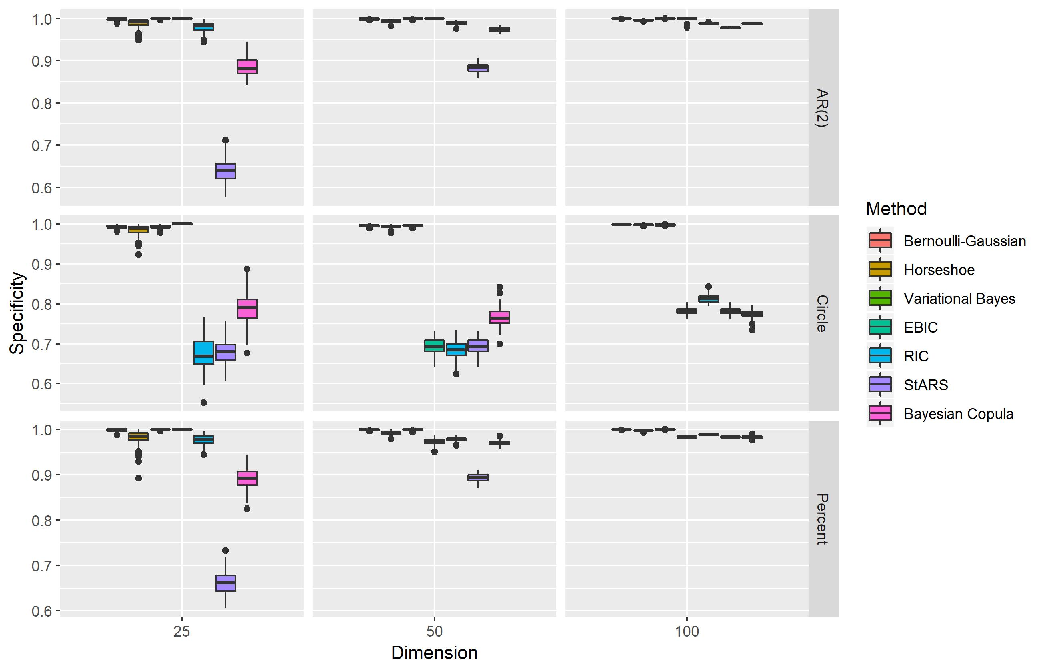
Next, we review how the methods perform when considering specificity. In Figure 2for all dimensions and AR(2) model, the three proposed methods, Bernoulli-Gaussian, Horseshoe, and Variational Bayes methods, as well as the EBIC method, perform the best. For the dimension and circle model, the three proposed methods, Bernoulli-Gaussian, Horseshoe, and Variational Bayes methods, as well as the EBIC method, perform the best. For the and dimensions and the circle model, the three proposed methods, Bernoulli-Gaussian, Horseshoe, and Variational Bayes methods, perform the best, outperforming all other methods. For the dimension and the 10% model, the three proposed methods, Bernoulli-Gaussian, Horseshoe, and Variational Bayes methods, as well as the EBIC method, perform the best. For the dimension and 5% model and the dimension and 2% model, the three proposed methods, Bernoulli-Gaussian, Horseshoe, and Variational Bayes methods, perform the best.
We consider the Matthews Correlation Coefficient to compare the overall performance of structure learning. In Figure 3for the and dimensions and the AR(2) model, the Bayesian Copula method performs the best and the Horseshoe method performs the second best. No edges were selected by the nonparanormal model using EBIC for the sparsity models of dimension and for the AR(2) model. For the dimension and the AR(2) model, the three proposed methods, Horseshoe, Bernoulli-Gaussian, and Variational Bayes methods, perform the best. For all dimensions of the circle model, the three proposed methods, Horseshoe, Bernoulli-Gaussian, and Variational Bayes methods, perform the best. Lastly, for the dimension and 10% model, the Horseshoe method performs the best, and the Bernoulli-Gaussian and RIC methods perform similarly and are the second best. For the and 5% model and and 2% model, the three proposed methods, Horseshoe, Bernoulli-Gaussian, and Variational Bayes methods, perform the best. Thus, compared to competing methods, when considering overall structure learning, the proposed methods outperform the competing methods except in the cases of and and AR(2) model.
Finally, in Figure 4we review the results of parameter estimation, using the scaled -loss, for the three proposed methods. We consider whether or not the transformation decreases the scaled -loss. For all three methods, the transformation functions resulted in a smaller scaled -loss, implying an improvement in parameter estimation. Overall, the Horseshoe method had a higher scaled -loss than the Bernoulli-Gaussian and Variational Bayes methods. In addition, overall, the Variational Bayes method had a similar or lower scaled -loss compared to the Bernoulli-Gaussian method.
Figures 1to 4display the results. The first three boxplots in the figures are the three proposed methods, Bernoulli-Gaussian, Horseshoe, and Variational Bayes, respectively. Note that Percent refers to the 10% model for dimension , model for dimension , and model for dimension .



9 Real Data Application
For the real data application, we consider the data set based on the GeneChip (Affymetrix) microarrays for the plant Arabidopsis thaliana originally referenced in (Wille et al. 2004). There are microarrays and genes from the isoprenoid pathway that are used. For pre-processing, the expression levels for each gene, for , are log-transformed. We study the associations among the genes using the Bayesian nonparanormal methods, the nonparanormal method of Liu et al. 2009, and the Bayesian copula graphical model of Mohammadi et al. 2017. These data are treated as multivariate Gaussian originally in (Wille et al. 2004).
Using the same set-up as in the simulation study, we fit the Bayesian copula graphical model using the BDGraph package and we fit the nonparanormal graphical model using the huge package. The BDGraph package selected 211 edges using Bayesian model averaging. The huge package using the RIC selection resulted in 140 edges and using the StARS method resulted in 209 edges. The EBIC-selected model results in no edges.
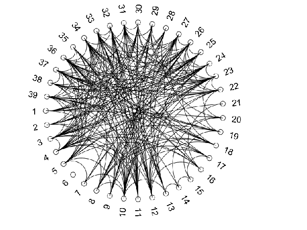
In order to construct the graphical models using our methods which use B-spline transformations, we converted the observations to be between 0 and 1 using the equation . The variational Bayes method results in 98 edges, the horseshoe prior based method results in 257 edges, and the Bernoulli-Gaussian prior based method results in 102 edges. For , convergence of the variational Bayes method can be achieved in about 26 minutes, the horseshoe prior based method in about 47 minutes for a given , and the Bernoulli-Gaussian prior based method in about 52 minutes on a laptop computer with Windows operating system, 2.8 GHz of CPU, and 28 GB of RAM. Figure 5shows the graphs of our proposed methods and Figure 6shows the graphs of the existing methods.
Since we use a sparsity prior for each of the graphs, we consider the sparsity to compare the performance of the graphs. The Variational Bayes and Bernoulli-Gaussian prior methods result in the sparsest graphs. The Horseshoe prior method results in the densest graph. Out of the three proposed methods, the horseshoe prior method is the most sensitive method, so it appears for this data set, it is selecting more edges than the other models. The Variational Bayes method is the fastest method out of the three proposed methods. The Variational Bayes and Bernoulli-Gaussian prior methods proposed in this paper give sparser graphs than the Gaussian copula graphical model method, which uses a G-Wishart prior on the precision matrix. Sparse graphs can aid in simpler scientific interpretation and could be used for further exploration, such as understanding the mechanisms involved in the isoprenoid pathway.




10 Discussion
We have introduced a Bayesian regression method to construct graphical models for continuous data that do not rely on a normality assumption. The method assumes the nonparanormal structure, that under some unknown monotone transformations, the original observation vector reduces to a multivariate normal vector. The precision matrix of the transformed observations can be used to learn the graphical structure of conditional independence of the original observations. We use a prior distribution on the underlying transformations through a finite random series of B-splines with increasing coefficients that are given a multivariate truncated normal prior. We incorporate the positive definiteness constraint on the precision matrix of the transformed variables by utilizing the Cholesky decomposition. We consider two different priors based on the Cholesky decomposition, the Bernoulli-Gaussian prior and the horseshoe prior, and we impose a sparsity constraint. We use a variational Bayesian algorithm to learn the conditional independence relations more efficiently as well as use a traditional Gibbs sampling approach. The variational Bayesian approach and the approaches using Bernoulli-Gaussian and horseshoe priors result in most cases with better overall structure learning, measured using the Matthews correlation coefficient, than competing methods. In addition, the variational Bayesian algorithm performs similarly to the proposed methods in terms of overall structure learning and parameter estimation. Thus, it appears that information is not lost with the variational Bayesian algorithm and we have the potential to speed up the estimation of the Bayesian nonparanormal graphical model. Lastly, when comparing the horseshoe to the Bernoulli-Gaussian methods, the horseshoe method has higher sensitivity and the Bernoulli-Gaussian methods perform similarly to the horseshoe in terms of specificity and overall structure learning and better in terms of parameter estimation.
Bayesian nonparanormal graphical models are flexible. They can be used to estimate the elements of the precision matrix directly or via a Cholesky decomposition. Researchers can try different sparsity priors on the precision matrix based on their interests and needs. In addition, researchers can use a fully Bayesian approach to learn the graphical structure or employ a partially Bayesian approach to increase the speed in learning the structure without sacrificing much in quality. The Bernoulli-Gaussian prior, used in the variational Bayesian method and the traditional Bayesian approach, resulted in the sparsest graphs using real data, which might be useful for researchers who would like greater variable reduction for data exploration.
References
- Armagan et al. (2013)
Armagan, A., D. B. Dunson, and J. Lee, 2013: Generalized double Pareto
shrinkage. Statistica Sinica, 23, no. 1, 119–143,
doi:10.5705/ss.2011.048.
URL http://www3.stat.sinica.edu.tw/statistica/j23n1/J23N16/J23N16.html - Banerjee et al. (2008)
Banerjee, O., L. El Ghaoui, and A. d’Aspremont, 2008: Model selection through
sparse maximum likelihood estimation for multivariate Gaussian or binary
data. Journal of Machine Learning Research, 9, 485–516.
URL http://dl.acm.org/citation.cfm?id=1390681.1390696 - Banerjee and Ghosal (2015)
Banerjee, S. and S. Ghosal, 2015: Bayesian structure learning in graphical
models. Journal of Multivariate Analysis, 136, 147 – 162,
doi:http://dx.doi.org/10.1016/j.jmva.2015.01.015.
URL http://www.sciencedirect.com/science/article/pii/S0047259X15000202 - Berger and Barbieri (2004)
Berger, J. O. and M. M. Barbieri, 2004: Optimal predictive model selection.
The Annals of Statistics, 32, no. 3, 870–897,
doi:10.1214/009053604000000238.
URL http://projecteuclid.org/euclid.aos/1085408489 - Bhattacharya et al. (2016) Bhattacharya, A., A. Chakraborty, and B. K. Mallick, 2016: Fast sampling with Gaussian scale-mixture priors in high-dimensional regression. Biometrika, 103, no. 4, 985–991, doi:10.1093/biomet/asw042.
- Bhattacharya et al. (2015)
Bhattacharya, A., D. Pati, N. S. Pillai, and D. B. Dunson, 2015:
Dirichlet-Laplace priors for optimal shrinkage. Journal of the
American Statistical Association, 110, no. 512, 1479–1490,
doi:10.1080/01621459.2014.960967.
URL http://www.tandfonline.com/doi/full/10.1080/01621459.2014.960967 - Bishop (2006) Bishop, C. M., 2006: Pattern Recognition and Machine Learning (Information Science and Statistics). Springer-Verlag New York, Inc., Secaucus, NJ, USA.
- Blei et al. (2017)
Blei, D. M., A. Kucukelbir, and J. D. McAuliffe, 2017: Variational Inference:
A Review for Statisticians. Journal of the American Statistical
Association, 112, no. 518, 859–877,
doi:10.1080/01621459.2017.1285773.
URL http://dx.doi.org/10.1080/01621459.2017.1285773 - Carvalho et al. (2009) Carvalho, C. M., N. G. Polson, and J. G. Scott, 2009: Handling sparsity via the horseshoe. JMLR Workshop and Conference Proceedings, volume 5, 73–80.
- Chen et al. (2011) Chen, M., H. Wang, X. Liao, and L. Carin, 2011: Bayesian learning of sparse Gaussian graphical models. Working paper.
- Dahl et al. (2005)
Dahl, J., V. Roychowdhury, and L. Vandenberghe, 2005: Maximum likelihood
estimation of Gaussian graphical models: numerical implementation and
topology selection. Technical report. University of California, Los
Angeles.
URL http://www.seas.ucla.edu/~vandenbe/publications/covsel1.pdf - Dahl et al. (2008)
Dahl, J., L. Vandenberghe, and V. Roychowdhury, 2008: Covariance selection for
nonchordal graphs via chordal embedding. Optimization Methods and
Software, 23, no. 4, 501–520, doi:10.1080/10556780802102693.
URL http://www.tandfonline.com/doi/abs/10.1080/10556780802102693 - d’Aspremont et al. (2008)
d’Aspremont, A., O. Banerjee, and L. El Ghaoui, 2008: First-order methods for
sparse covariance selection. SIAM Journal on Matrix Analysis and
Applications, 30, no. 1, 56–66, doi:10.1137/060670985.
URL http://epubs.siam.org/doi/abs/10.1137/060670985 - Dobra and Lenkoski (2011)
Dobra, A. and A. Lenkoski, 2011: Copula Gaussian graphical models and their
application to modeling functional disability data. The Annals of
Applied Statistics, 5, no. 2A, 969–993, doi:10.1214/10-AOAS397.
URL http://projecteuclid.org/euclid.aoas/1310562213 - Foygel and Drton (2010)
Foygel, R. and M. Drton, 2010: Extended Bayesian information criteria for
Gaussian graphical models. Advances in Neural Information
Processing Systems 23, 604–612.
URL http://books.nips.cc/papers/files/nips23/NIPS2010_0060.pdf - Friedman et al. (2008)
Friedman, J., T. Hastie, and R. Tibshirani, 2008: Sparse inverse covariance
estimation with the graphical lasso. Biostatistics, 9, no. 3,
432–441, doi:10.1093/biostatistics/kxm045.
URL http://biostatistics.oxfordjournals.org/cgi/doi/10.1093/biostatistics/kxm045 - Gan et al. (2019)
Gan, L., N. N. Narisetty, and F. Liang, 2019: Bayesian Regularization for
Graphical Models With Unequal Shrinkage. Journal of the
American Statistical Association, 114, no. 527, 1218–1231,
doi:10.1080/01621459.2018.1482755.
URL https://www.tandfonline.com/doi/full/10.1080/01621459.2018.1482755 - Jordan et al. (1999)
Jordan, M. I., Z. Ghahramani, T. S. Jaakkola, and L. K. Saul, 1999: An
introduction to variational methods for graphical models. Machine
Learning, 37, no. 2, 183–233, doi:10.1023/A:1007665907178.
URL https://doi.org/10.1023/A:1007665907178 - Khondker et al. (2013) Khondker, Z. S., H. Zhu, H. Chu, W. Lin, and J. G. Ibrahim, 2013: The Bayesian covariance lasso. Statistics and Its Interface, 6, no. 2, 243–259.
- Kuismin and Sillanpää (2016)
Kuismin, M. and M. J. Sillanpää, 2016: Use of Wishart prior and simple
extensions for sparse precision matrix estimation. PLOS ONE, 11, no. 2, e0148171, doi:10.1371/journal.pone.0148171.
URL http://dx.plos.org/10.1371/journal.pone.0148171 - Li and Pati (2017)
Li, H. and D. Pati, 2017: Variable selection using shrinkage priors. Computational Statistics & Data Analysis, 107, 107–119,
doi:10.1016/j.csda.2016.10.008.
URL http://linkinghub.elsevier.com/retrieve/pii/S0167947316302353 - Li et al. (2019)
Li, Z. R., T. H. McComick, and S. J. Clark, 2019: Using Bayesian Latent
Gaussian Graphical Models to Infer Symptom Associations in
Verbal Autopsies. Bayesian Analysis, doi:10.1214/19-BA1172.
URL https://projecteuclid.org/euclid.ba/1569290444 - Li and McCormick (2019)
Li, Z. R. and T. H. McCormick, 2019: An Expectation Conditional
Maximization Approach for Gaussian Graphical Models. Journal
of Computational and Graphical Statistics, 28, no. 4, 767–777,
doi:10.1080/10618600.2019.1609976.
URL https://www.tandfonline.com/doi/full/10.1080/10618600.2019.1609976 - Liu et al. (2012)
Liu, H., F. Han, M. Yuan, J. Lafferty, and L. Wasserman, 2012: High-dimensional
semiparametric Gaussian copula graphical models. The Annals of
Statistics, 40, no. 4, 2293–2326.
URL http://www.jstor.org/stable/41806536 - Liu et al. (2009)
Liu, H., J. D. Lafferty, and L. A. Wasserman, 2009: The nonparanormal:
semiparametric estimation of high dimensional undirected graphs. Journal
of Machine Learning Research, 10, 2295–2328.
URL http://jmlr.csail.mit.edu/papers/volume10/liu09a/liu09a.pdf - Liu et al. (2010)
Liu, H., K. Roeder, and L. Wasserman, 2010: Stability approach to
regularization selection (StARS) for high dimensional graphical models.
Advances in Neural Information Processing Systems 23, USA,
1432–1440.
URL http://dl.acm.org/citation.cfm?id=2997046.2997056 - Lu (2009)
Lu, Z., 2009: Smooth optimization approach for sparse covariance selection.
SIAM Journal on Optimization, 19, no. 4, 1807–1827,
doi:10.1137/070695915.
URL http://epubs.siam.org/doi/10.1137/070695915 - Lysen (2009)
Lysen, S., 2009: Permuted inclusion criterion: a variable selection
technique. Ph.D. thesis, Publicly Accessible Penn Dissertations, 28.
URL http://repository.upenn.edu/edissertations/28 - Mazumder and Hastie (2012a) Mazumder, R. and T. Hastie, 2012a: Exact covariance thresholding into connected components for large-scale graphical lasso. Journal of Machine Learning Research, 13, 781–794.
- Mazumder and Hastie (2012b)
— 2012b: The graphical lasso: new insights and alternatives.
Electronic Journal of Statistics, 6, no. 0, 2125–2149,
doi:10.1214/12-EJS740.
URL http://projecteuclid.org/euclid.ejs/1352470831 - Meinshausen and Buhlmann (2006)
Meinshausen, N. and P. Buhlmann, 2006: High-dimensional graphs and variable
selection with the lasso. The Annals of Statistics, 34, no. 3,
1436–1462, doi:10.1214/009053606000000281.
URL http://projecteuclid.org/Dienst/getRecord?id=euclid.aos/1152540754/ - Mohammadi et al. (2017)
Mohammadi, A., F. Abegaz, E. van den Heuvel, and E. C. Wit, 2017: Bayesian
modelling of Dupuytren disease by using Gaussian copula graphical models.
Journal of the Royal Statistical Society: Series C (Applied
Statistics), 66, no. 3, 629–645, doi:10.1111/rssc.12171.
URL http://doi.wiley.com/10.1111/rssc.12171 - Mohammadi and Wit (2015) Mohammadi, A. and E. C. Wit, 2015: Bayesian structure learning in sparse Gaussian graphical models. Bayesian Analysis, 10, no. 1, 109–138, doi:10.1214/14-BA889.
- Mohammadi and Wit (2019)
Mohammadi, R. and E. C. Wit, 2019: BDgraph : An R
Package for Bayesian Structure Learning in Graphical Models. Journal of Statistical Software, 89, no. 3,
doi:10.18637/jss.v089.i03.
URL http://www.jstatsoft.org/v89/i03/ - Mulgrave and Ghosal (2020)
Mulgrave, J. J. and S. Ghosal, 2020: Bayesian Inference in Nonparanormal
Graphical Models. Bayesian Analysis, 15, no. 2, 449–475,
doi:10.1214/19-BA1159.
URL https://projecteuclid.org/euclid.ba/1559721629 - Neville et al. (2014)
Neville, S. E., J. T. Ormerod, and M. P. Wand, 2014: Mean field variational
Bayes for continuous sparse signal shrinkage: Pitfalls and remedies. Electronic Journal of Statistics, 8, no. 1, 1113–1151,
doi:10.1214/14-EJS910.
URL http://projecteuclid.org/euclid.ejs/1407415580 - Nguyen and Chiogna (2018)
Nguyen, T. K. H. and M. Chiogna, 2018: Structure learning of undirected
graphical models for count data. arXiv:1810.10854 [stat], arXiv:
1810.10854.
URL http://arxiv.org/abs/1810.10854 - Ormerod et al. (2017)
Ormerod, J. T., C. You, and S. Müller, 2017: A variational Bayes approach to
variable selection. Electronic Journal of Statistics, 11, no.
2, 3549–3594, doi:10.1214/17-EJS1332.
URL https://projecteuclid.org/euclid.ejs/1507255614 - Pakman and Paninski (2014)
Pakman, A. and L. Paninski, 2014: Exact Hamiltonian Monte Carlo for
truncated multivariate Gaussians. Journal of Computational and
Graphical Statistics, 23, no. 2, 518–542,
doi:10.1080/10618600.2013.788448.
URL http://www.tandfonline.com/doi/abs/10.1080/10618600.2013.788448 - Peterson et al. (2013)
Peterson, C., M. Vannucci, C. Karakas, W. Choi, L. Ma, and M. Maletic-Savatic,
2013: Inferring metabolic networks using the Bayesian adaptive graphical
lasso with informative priors. Statistics and Its Interface, 6,
no. 4, 547–558, doi:10.4310/SII.2013.v6.n4.a12.
URL http://www.intlpress.com/site/pub/pages/journals/items/sii/content/vols/0006/0004/a012/ - Peterson et al. (2016)
Peterson, C. B., F. C. Stingo, and M. Vannucci, 2016: Joint Bayesian variable
and graph selection for regression models with network-structured predictors.
Statistics in Medicine, 35, no. 7, 1017–1031,
doi:10.1002/sim.6792.
URL http://doi.wiley.com/10.1002/sim.6792 - Pitt et al. (2006)
Pitt, M., D. Chan, and R. Kohn, 2006: Efficient Bayesian inference for
Gaussian copula regression models. Biometrika, 93, no. 3,
537–554.
URL http://www.jstor.org/stable/20441306 - Pourahmadi (2011)
Pourahmadi, M., 2011: Covariance estimation: The GLM and regularization
perspectives. Statistical Science, 26, no. 3, 369–387,
doi:10.1214/11-STS358.
URL http://projecteuclid.org/euclid.ss/1320066926 - Rothman et al. (2008)
Rothman, A. J., P. J. Bickel, E. Levina, and J. Zhu, 2008: Sparse permutation
invariant covariance estimation. Electronic Journal of Statistics,
2, no. 0, 494–515, doi:10.1214/08-EJS176.
URL http://projecteuclid.org/euclid.ejs/1214491853 - Scheinberg et al. (2010)
Scheinberg, K., S. Ma, and D. Goldfarb, 2010: Sparse inverse covariance
selection via alternating linearization methods. Proceedings of the 23rd
International Conference on Neural Information Processing Systems
- Volume 2, Curran Associates Inc., USA, NIPS’10, 2101–2109.
URL http://dl.acm.org/citation.cfm?id=2997046.2997130 - Soussen et al. (2011)
Soussen, C., J. Idier, D. Brie, and J. Duan, 2011: From Bernoulli-Gaussian
deconvolution to sparse signal restoration. IEEE Transactions on Signal
Processing, 59, no. 10, 4572–4584, doi:10.1109/TSP.2011.2160633.
URL http://ieeexplore.ieee.org/document/5930380/ - van der Pas et al. (2014)
van der Pas, S. L., B. J. K. Kleijn, and A. W. van der Vaart, 2014: The
horseshoe estimator: posterior concentration around nearly black vectors.
Electronic Journal of Statistics, 8, no. 2, 2585–2618,
doi:10.1214/14-EJS962.
URL https://projecteuclid.org:443/euclid.ejs/1418134265 - Wainwright and Jordan (2007)
Wainwright, M. J. and M. I. Jordan, 2007: Graphical models, exponential
families, and variational inference. Foundations and Trends® in Machine
Learning, 1, no. 1–2, 1–305, doi:10.1561/2200000001.
URL http://www.nowpublishers.com/article/Details/MAL-001 - Wang (2012)
Wang, H., 2012: Bayesian graphical lasso models and efficient posterior
computation. Bayesian Analysis, 7, no. 4, 867–886,
doi:10.1214/12-BA729.
URL http://projecteuclid.org/euclid.ba/1354024465 - Wang (2015)
— 2015: Scaling it up: stochastic search structure learning in graphical
models. Bayesian Analysis, 10, no. 2, 351–377,
doi:10.1214/14-BA916.
URL http://projecteuclid.org/euclid.ba/1422884978 - Wille et al. (2004)
Wille, A., P. Zimmermann, E. Vranová, A. Fürholz, O. Laule, S. Bleuler,
L. Hennig, A. Prelić, P. von Rohr, L. Thiele, E. Zitzler, W. Gruissem, and
P. Bühlmann, 2004: Sparse graphical Gaussian modeling of the isoprenoid
gene network in Arabidopsis thaliana. Genome Biology, 5, no. 11, R92–R92, doi:10.1186/gb-2004-5-11-r92.
URL http://www.ncbi.nlm.nih.gov/pmc/articles/PMC545783/ - Williams et al. (2018)
Williams, D. R., J. Piironen, A. Vehtari, and P. Rast, 2018: Bayesian
estimation of Gaussian graphical models with projection predictive
selection. arXiv preprint arXiv:1801.05725.
URL https://arxiv.org/abs/1801.05725 - Witten et al. (2011)
Witten, D. M., J. H. Friedman, and N. Simon, 2011: New insights and faster
computations for the graphical lasso. Journal of Computational and
Graphical Statistics, 20, no. 4, 892–900,
doi:10.1198/jcgs.2011.11051a.
URL http://www.tandfonline.com/doi/abs/10.1198/jcgs.2011.11051a - Wong et al. (2013)
Wong, E., S. P. Awate, and P. T. Fletcher, 2013: Adaptive sparsity in
Gaussian graphical models. Proceedings of the 30th International
Conference on International Conference on Machine Learning -
Volume 28, JMLR.org, Atlanta, GA, USA, ICML’13, I–311–I–319.
URL http://dl.acm.org/citation.cfm?id=3042817.3042854 - Yuan and Lin (2007)
Yuan, M. and Y. Lin, 2007: Model selection and estimation in the Gaussian
graphical model. Biometrika, 94, no. 1, 19–35,
doi:10.1093/biomet/asm018.
URL http://biomet.oxfordjournals.org/cgi/doi/10.1093/biomet/asm018 - Zhang (2020)
Zhang, Q., 2020: Testing Differential Gene Networks under Nonparanormal
Graphical Models with False Discovery Rate Control. Genes, 11, no. 2, 167, doi:10.3390/genes11020167.
URL https://www.mdpi.com/2073-4425/11/2/167 - Zhao et al. (2015)
Zhao, T., X. Li, H. Liu, K. Roeder, J. Lafferty, and L. Wasserman, 2015: huge:
high-dimensional undirected graph estimation. R package version 1.2.7.
URL http://CRAN.R-project.org/package=huge
Acknowledgments
We would like to acknowledge support for this project for the first author from the National Science Foundation (NSF) Graduate Research Fellowship Program Grant No. DGE-1252376, the National Institutes of Health (NIH) training grant GM081057 and NSF grant DMS-1732842. Secondly, we would like to acknowledge partial support for this project for the second author by NSF grant DMS-1510238.
Financial disclosure
None reported.
Conflict of interest
The authors declare no potential conflict of interests.
Appendix A Horseshoe Posterior
The joint posterior distribution is,
Then the corresponding conditional posterior distributions are given by
Since sampling the can be expensive for large , we use an exact sampling algorithm for Gaussian priors based on data augmentation (Bhattacharya et al. 2016).
Appendix B Bernoulli-Gaussian Posterior
The joint posterior distribution is
Then the corresponding conditional posterior distributions are given by
where , and .
Again, to sample we used an exact sampling algorithm for Gaussian priors that invokes data augmentation (Bhattacharya et al. 2016).
- (a)
Initialize with where
- (b)
for do
- •
- •
- •
- •
- •
- •
- •
- •
for do
- –
- –
- –
- •
end for
- •
- •
- (c)
end for
- (d)
- (e)
Repeat (b)–(d) until
- (a)
Sample where
- (i)
Sample and , where
- (ii)
set , where
- (iii)
solve for in , where
- (iv)
set
- (i)
- (b)
Sample
- (c)
Sample
- (d)
Sample
- (e)
Sample
- (f)
Sample
| (6) |
- (a)
Sample , where
- (i)
Sample and , where ;
- (ii)
set , where ;
- (iii)
solve for in , where ;
- (iv)
set .
- (i)
- (b)
Sample
- (c)
Sample .
Appendix C GitHub Repository
https://github.com/jnj2102/BayesianRegressionApproach
The code used to run the methods described in this paper are available on GitHub.