Time Evolution of Entanglement Negativity from Black Hole InteriorsarXiv: 1812.04424

\justify

Over the last few years quantum entanglement has emerged as a central issue in the study of diverse physical phenomena ranging from quantum many-body systems in out-of-equilibrium to the process of black hole formation and the information loss paradox. The entanglement for a bipartite pure state is characterized by the entanglement entropy which is the von Neumann entropy of the reduced density matrix. In $(1+1)$-dimensional conformal field theories ($CFT_{1+1}$) the entanglement entropy may be computed through a replica technique as described in Calabrese:2004eu; Calabrese:2009qy. However entanglement entropy fails to characterize mixed state entanglement as it typically involves correlations irrelevant to the entanglement of the specific mixed state. This subtle issue was addressed in quantum information theory by Vidal and Werner in PhysRevA.65.032314 where the authors proposed a computable measure termed as entanglement negativity which characterized the upper bound on the distillable entanglement for the mixed state¹¹ 1 It was demonstrated by Plenio in Plenio:2005cwa that this entanglement measure was not convex but was an entanglement monotone under local operations and classical communication (LOCC).. The entanglement negativity is defined as the logarithm of the trace norm of the partially transposed density matrix with respect to a subsystem. In a series of interesting communications the authors in Calabrese:2012ew; Calabrese:2012nk; Calabrese:2014yza described the computation of the entanglement negativity for bipartite mixed states in a $CFT_{1+1}$ through a suitable replica technique.

A holographic characterization of the entanglement entropy in $CFT$s was proposed by Ryu and Takayanagi Ryu:2006bv; Ryu:2006ef through the $AdS/CFT$ correspondence. According to their conjecture the universal part of the entanglement entropy of a subsystem in a dual $d$-dimensional conformal field theories ($CFT_{d}$) was proportional to the area of a co-dimension two static minimal surface in the bulk $AdS_{d+1}$ geometry homologous to the subsystem. Naturally, this led to intense research activity in various aspects of entanglement related issues in holographic $CFT$s Takayanagi:2012kg; Nishioka:2009un; Nishioka:2018khk; e12112244; Blanco:2013joa; Fischler2013; Fischler:2012uv; Chaturvedi:2016kbk (and references therein). In a series of interesting communications, a proof of this conjecture was developed from a bulk perspective, initially in the context of $AdS_{3}/CFT_{2}$ and later generalized to the $AdS_{d+1}/CFT_{d}$ scenario Fursaev:2006ih; Headrick:2010zt; Faulkner:2013yia; Casini:2011kv; Lewkowycz:2013nqa. A covariant extension of the RT conjecture was proposed for the entanglement entropy of a subsystem in a $CFT_{d}$ dual to a non static bulk $AdS_{d+1}$ geometry in Hubeny:2007xt and the corresponding proof in Dong:2016hjy.

The above developments naturally lead to the interesting question of a holographic characterization of the entanglement negativity for bipartite pure and mixed states in dual $CFT$s Rangamani:2014ywa; Perlmutter:2015vma. In the recent past two of the present authors (VM and GS) in a collaboration, proposed a holographic construction for the entanglement negativity of bipartite pure and mixed states in a dual $CFT_{1+1}$ through $AdS_{3}/CFT_{2}$ framework and its covariant extension Chaturvedi:2016rcn; Chaturvedi:2016opa. This construction was rigorously substantiated through a large central charge analysis employing the monodromy technique in Malvimat:2017yaj, although a bulk proof for this conjecture along the lines of Faulkner:2013yia is an outstanding issue. Subsequently, their proposal was also extended to higher dimensions in the context of the $AdS_{d+1}/CFT_{d}$ scenario in Chaturvedi:2016rft. It should be mentioned here that a proof of the higher dimensional extension for the holographic entanglement negativity conjecture described above from a bulk perspective along the lines of Lewkowycz:2013nqa is also an outstanding non trivial open issue. Subsequent to this in Jain:2017aqk; Jain:2017uhe, a holographic characterization for the entanglement negativity of a mixed state of adjacent intervals in $CFT_{1+1}$s dual to bulk $AdS_{3}$ geometries, and its covariant generalization was proposed. A higher dimensional generalization of the above holographic construction for such mixed states of adjacent subsystems in a $CFT_{d}$ dual to bulk $AdS_{d+1}$ geometry, was subsequently advanced in Jain:2017xsu; Jain:2018bai. Furthermore very recently a holographic construction for the entanglement negativity of mixed states of two disjoint intervals in a dual $CFT_{1+1}$ and its covariant extension has been developed in Malvimat:2018txq; Malvimat:2018ood.

In a different context the study of out of equilibrium quantum systems to elucidate their dynamical evolution has witnessed a strong surge of interest in recent times Calabrese:2005in; Calabrese:2009qy; calabrese2016quantum; Wen:2018svb; Wen:2015qwa. One of the processes through which a quantum system may be placed in an out of equilibrium configuration is a quantum quench. In a global quench scenario a quantum system is initially prepared in the ground state of a translationally invariant Hamiltonian $H_{0}$ and is then allowed to evolve unitarily with respect to another Hamiltonian $H$, where $H$ and $H_{0}$ are related to each other through an experimentally tunable parameter. In a $CFT_{1+1}$ the resulting state after a global quench may be regarded as a boundary state (B-state) as it is translational and conformal invariant below the energy scale of the global quench. The corresponding time evolution of the entanglement entropy after a global quench for a subsystem maybe computed through the replica technique Calabrese:2005in; Calabrese:2009qy; calabrese2016quantum in a $CFT_{1+1}$. It was shown that in the spacetime scaling limit²² 2 In the spacetime scaling limit the time $t$ and the interval length $\ell$ are much larger than the microscopic length and time scale in the theory Coser:2014gsa; PhysRevA.78.010306; PhysRevLett.106.227203; Calabrese:2009qy. the entanglement entropy grows linearly for early times and is rendered extensive beyond a certain value of time. It is possible to describe such a time evolution of the entanglement following a global quench, through a quasi-particle scenario for the entanglement propagation Calabrese:2005in; calabrese2016quantum; Calabrese:2007rg; Calabrese:2006rx. In this instance the initial state which is at a higher energy relative to the ground state of the post-quench Hamiltonian, acts as a source of quasi-particle excitations.

Following the developments described above the corresponding time evolution of the entanglement negativity for mixed states of two adjacent and disjoint intervals in a $CFT_{1+1}$ following a global quench was investigated in Coser:2014gsa. Very interestingly they demonstrated that similar to the entanglement entropy, the time evolution of entanglement negativity also admits of a quasi-particle explanation for the mixed state entanglement propagation. However it was observed that the initial increase in the entanglement negativity occurs slightly after the time predicted by the quasi-particle picture as a consequence of the late birth of entanglement in a lattice system which disappears in the continuum limit Coser:2014gsa.

On the other hand the time evolution of holographic entanglement entropy after a global quench in a $CFT_{1+1}$ dual to a bulk Vaidya-AdS geometry describing black hole formation has been extensively studied in the literature Hubeny:2007xt; AbajoArrastia:2010yt; Aparicio:2011zy; Albash:2010mv; Balasubramanian:2010ce; Balasubramanian:2011ur; Allais:2011ys; Liu:2013iza; Liu:2013qca; Ugajin:2013xxa; Liu:2018crr; Anous:2017tza. Although as discussed in Hartman:2013qma, the precise holographic dual for the global quench scenario where the initial state is a time dependent pure boundary state (B-state) in a $CFT_{1+1}$ Calabrese:2005in, is the eternal black hole geometry sliced in half by an end-of-the-world (ETW) brane or simply a single sided black hole³³ 3 Recently in Cooper:2018cmb, a somewhat similar bulk configuration is considered where the end-of-the-world (ETW) brane is extended into the second asymptotic region.. It is well known from Israel:1976ur; Maldacena:2001kr; Hartman:2013qma that the eternal black hole is dual to the thermofield double state in a $CFT$. These involve two-sided Penrose diagram and are static under time evolution as the time directions are taken to be opposite for the two sides. However, the time dependence may be introduced for this geometry by considering forward time evolution for both the exterior regions of the Penrose diagram.

The computation of the corresponding holographic entanglement entropy for a subsystem $A$ in a $CFT$ for the thermofield double state dual to the bulk eternal black hole geometry requires the consideration of the subsystem in question on both sides of the Penrose diagram. The entanglement entropy may then be computed from the area of the extremal surface anchored on both the subsystems in accordance with the RT and the HRT conjectures. It was observed in Hartman:2013qma that the eternal black hole in $AdS_{3}$ may be mapped to a BTZ black brane geometry. In this case it was demonstrated that for early times the extremal surface (geodesic) passes through the interior region of the black brane geometry connecting one asymptotic region to the other. Hence the linear growth of the entanglement entropy was related to the growth of the extremal surface along the nice slice⁴⁴ 4 Nice slices are spacelike surfaces with small curvatures where any matter moves with modest velocity in the local frame defined by these slices Polchinski:1995ta. in the interior region of the black brane. For late times the extremal surface reduces to a static minimal surface located exterior to the horizon and the entanglement entropy is rendered extensive Hartman:2013qma. It is argued in Hartman:2013qma that the holographic entanglement entropy of the configuration in question after a global quench scenario Calabrese:2005in is just half of the corresponding holographic entanglement entropy for the eternal black hole geometry.

Quite naturally the developments described above lead to the interesting issue of a holographic characterization for the time evolution of the entanglement negativity for mixed state configurations following a global quench in a dual $CFT_{1+1}$. As mentioned earlier the correct holographic dual for the global quench scenario is described by an eternal black hole geometry sliced in half by an ETW brane. Hence to this end it is required to obtain the holographic entanglement negativity for such mixed states from the dual eternal black hole geometry.

In this article we address the significant issue described above and investigate the time evolution of the holographic entanglement negativity for mixed state configurations of disjoint and adjacent intervals following a global quench in a $CFT_{1+1}$. As described in Coser:2014gsa the entanglement negativity for the above configurations in a $CFT_{1+1}$ with a global quench involve the corresponding four and three point twist correlators on a strip. It is significant to mention here that the universal parts of these twist correlators relevant in the space time scaling limit factorize into products of various two point twist correlators on a strip. This leads to an expression for the entanglement negativity of these configurations which involve a specific algebraic sum of the corresponding entanglement entropies of appropriate intervals and their combinations. The holographic entanglement negativity for the above configurations may then be computed from the prescription for the entanglement entropies described in Hartman:2013qma for a bulk eternal black hole geometry sliced in half by an ETW brane. From our computations we observe an interesting structure of bulk geodesics connecting the two asymptotic regions which evolves with time to a geodesic structure that is located only in the exterior region. The corresponding holographic entanglement negativity for the mixed state configurations following a global quench in a $CFT_{1+1}$ is then given by half of that obtained for the eternal black hole geometry. It is observed that the holographic entanglement negativity for the mixed state configurations in question exhibits a linear growth during the initial part of its time evolution. For late times it decreases linearly with an identical slope from a maximum value and goes to zero after a certain value of time which indicates the process of thermalization and black hole formation in the bulk Calabrese:2006rx; Balasubramanian:2010ce; Balasubramanian:2011ur; Buchel:2013lla. Remarkably the holographic entanglement negativity of the mixed state configurations in question, computed through our construction exactly reproduces the corresponding $CFT_{1+1}$ replica technique results following a global quench as described in Coser:2014gsa.

This article is organized as follows. In Sec. (2), we briefly review the time evolution of entanglement entropy for a single interval after a global quench in a $CFT_{1+1}$. The evolution of entanglement negativity for two disjoint and adjacent intervals after a global quench in a $CFT_{1+1}$ is reviewed in Sec. (3). In Sec. (4) we review the time evolution of the corresponding holographic entanglement entropy for a single interval from a dual bulk eternal black hole geometry. In the next Sec. (5), we establish our holographic construction for the time evolution of the entanglement negativity for two disjoint and adjacent intervals from the dual bulk eternal black hole geometry. The holographic entanglement negativity for the mixed state configurations following a global quench is then given by half of that obtained for the eternal black hole geometry and exactly matches with the corresponding $CFT_{1+1}$ replica technique results. We then present a summary and our conclusions in the final Sec. (6).

In this section we briefly review the time evolution of the entanglement entropy following a global quench as described in Calabrese:2005in; Calabrese:2009qy; calabrese2016quantum; Coser:2014gsa. In a global quench scenario, the system is initially prepared in a pure state $|\psi_{0}\rangle$ which is the ground state of a Hamiltonian $H_{0}$ at time $t=0$. For time $t>0$ the same system is allowed to evolve unitarily with respect to another Hamiltonian $H$, where $H$ and $H_{0}$ are related to each other by an experimentally tunable parameter. The unitary evolution of the density matrix $\rho_{0}=|\psi_{0}\rangle\langle\psi_{0}|$ for $t>0$ is governed by the post-quenched Hamiltonian $H$ as

$$\rho(t)=|\psi(t)\rangle\langle\psi(t)|=e^{-iHt}|\psi_{0}\rangle\langle\psi_{0}|e^{iHt},$$

(1)

where $\rho(t)$ is the density matrix at a time $t$ which is always in a pure state as a consequence of unitary evolution. The entanglement entropy of a subsystem $A$ is obtained as the von Neumann entropy of the reduced density matrix $\rho_{A}(t)={\rm Tr}_{B}\rho(t)$ where $B=A^{c}$ represents the rest of the system, which is given as

$$S_{A}(t)=-\mathrm{Tr}\left(\rho_{A}(t)\ln\rho_{A}(t)\right).$$

(2)

In a $CFT_{1+1}$ for simplicity the initial state may be chosen as $|\psi_{0}\rangle=e^{-{\tau_{0}H}/{4}}|B\rangle$ where $|B\rangle$ is a conformal invariant boundary state (B-state) and $\tau_{0}$ is the correlation length in the initial state. The entanglement entropy $S_{A}(t)$ may be obtained through a replica technique as follows

$$S_{A}(t)=-\lim_{n\to 1}\frac{\partial}{\partial n}{\rm Tr}\rho_{A}^{n}.$$

(3)

The quantity ${\rm Tr}\rho_{A}^{n}$ for a single interval $A$ of length $\ell$ as depicted in Fig. 1(a) in the $CFT_{1+1}$, is related to the two point twist correlator on a strip of width $2\tau_{0}$ as Calabrese:2005in; Calabrese:2009qy; calabrese2016quantum; Coser:2014gsa

$$\mathrm{Tr}\rho_{A}^{n}=\langle\,\mathcal{T}_{n}(w_{1})\bar{\mathcal{T}}_{n}(w_{2})\,\rangle_{\rm strip}\,,$$

(4)

where $w_{i}=u_{i}+\textrm{i}\tau\,$ are the complex coordinates on the strip ($u_{i}\in\mathbb{R}$ and $0<\tau<2\tau_{0}$). The above twist correlator may be obtained through a conformal map $z_{i}=\exp(\pi w_{i}/2\tau_{0})$ from the strip to the upper half plane (UHP) which is then given as

$$\langle\,\mathcal{T}_{n}(w_{1})\bar{\mathcal{T}}_{n}(w_{2})\,\rangle_{\rm strip}\,=\,c_{n}\left(\frac{\pi}{2\tau_{0}}\right)^{2\Delta_{n}}{\frac{1}{|(z_{1}-\bar{z}_{1})(z_{2}-\bar{z}_{2})\,\eta_{1,2}|^{\Delta_{n}}}}{\cal F}(\eta_{1,2})\,,$$

(5)

where $c_{n}$ is a constant and $\eta_{1,2}$ is the cross ratio, and the scaling dimension $\Delta_{n}$ of the twist operators $\mathcal{T}_{n}$ and $\bar{\mathcal{T}}_{n}$ is given as follows

$$\Delta_{n}=\frac{c}{12}\left(n-\frac{1}{n}\right).$$

(6)

The function ${\cal F}_{n}(\eta_{1,2})$ in eq. (5) is non-universal and depends on the full operator content of the theory. Note that only the limiting behavior of $\eta_{1,2}\to 0$ and $\eta_{1,2}\to 1$ are important and in these limits the non-universal function ${\cal F}_{n}(\{\eta_{1,2}\}$ is just a constant Coser:2014gsa. The entanglement entropy $S_{A}$ may now be obtained by utilizing eqs. (3) and (5) and considering the spacetime scaling limit ($t,\ell\gg\tau_{0}$), which is given as follows (see Coser:2014gsa for detailed computation)

$$S_{A}=\frac{\pi c}{6\tau_{0}}\big[t+q(t,\ell)\big]=\left\{\begin{array}[]{ll}\displaystyle\frac{\pi c}{6\tau_{0}}t&t<\ell/2\,,\\ \\ \displaystyle\frac{\pi c}{12\tau_{0}}\ell&t>\ell/2\,,\end{array}\right.$$

(7)

where the function $q(t,\ell)$ is defined as follows

$$q(t,\ell)\,\equiv\,\frac{\ell}{2}-\textrm{max}(t,\ell/2)\,=\,\left\{\begin{array}[]{ll}0&t<\ell/2\,,\\ \ell/2-t&t>\ell/2\,.\end{array}\right.$$

(8)

Note that the entanglement entropy $S_{A}$ increases linearly with time for $t<\ell/2$ and saturates to a thermal value beyond the time $t\sim\ell/2$. It may be observed that the entanglement entropy for large times is same as the thermal entropy of a mixed state at a large but finite temperature $T=\frac{1}{\beta}=\frac{1}{4\tau_{0}}$. This saturation to a thermal entropy at large times leads to the fascinating phenomena of $CFT$ thermalization as described inCalabrese:2006rx; Coser:2014gsa.

In this section we briefly recapitulate the evolution of the entanglement negativity for mixed states of two disjoint and adjacent intervals in a $CFT_{1+1}$ after a global quench scenario as described in Coser:2014gsa. As mentioned in the introduction, for a bipartite system $A=A_{1}\cup A_{2}$ in a mixed state, the entanglement between the subsystems $A_{1}$ and $A_{2}$ is characterized by the entanglement negativity, which is defined as PhysRevA.65.032314

$$\mathcal{E}=\ln\mathrm{Tr}|\rho_{A}^{T_{2}}|.$$

(9)

Here the partial transposed reduced density matrix $\rho_{A}^{T_{2}}$ is obtained as follows

$$\langle e^{(1)}_{i}e^{(2)}_{j}|\rho_{A}^{T_{2}}|e^{(1)}_{k}e^{(2)}_{l}\rangle=\langle e^{(1)}_{i}e^{(2)}_{l}|\rho_{A}|e^{(1)}_{k}e^{(2)}_{j}\rangle,$$

(10)

where $|e^{(1)}_{i}\rangle$ and $|e^{(2)}_{j}\rangle$ are the bases for the the Hilbert spaces $\mathcal{H}_{A_{1}}$ and $\mathcal{H}_{A_{2}}$ of the subsystems $A_{1}$ and $A_{2}$ respectively. In a $CFT_{1+1}$ the entanglement negativity is obtained through a suitable replica technique through the quantity $\mathrm{Tr}\big(\,\rho_{A}^{T_{2}}\big)^{n}$ for even $n=n_{e}$ and the analytic continuation to $n_{e}\to 1$ as follows Calabrese:2012ew; Calabrese:2012nk; Calabrese:2014yza

$$\mathcal{E}=\lim_{n_{e}\rightarrow 1}\ln\Big[\mathrm{Tr}\big(\,\rho_{A}^{T_{2}}\big)^{n_{e}}\Big]\,.$$

(11)

In this section we briefly review the holographic computation of the entanglement entropy for a single interval in a $CFT_{1+1}$ following a global quench in the $AdS_{3}/CFT_{2}$ framework. As described in Hartman:2013qma the correct holographic dual of the global quench scenario is given by the single sided eternal black hole obtained by slicing the Penrose diagram of the usual eternal black hole in half with an end of the world (ETW) brane. In this instance the minimal area extremal surfaces (geodesics for $AdS_{3}/CFT_{2}$) terminate on the ETW brane and the corresponding holographic entanglement entropy is just half of that obtained for the usual eternal black hole geometry.

In the above context we begin by reviewing the time evolution of the holographic entanglement entropy from a bulk eternal BTZ black hole geometry described by a two-sided Penrose diagram as depicted in Fig. 2. As described in Hartman:2013qma; Maldacena:1998bw this bulk geometry is dual to the two copies of the $CFT$ ($CFT_{R}\otimes CFT_{L}$), in the thermofield double state⁵⁵ 5 Thermofield double state is a purification of a mixed state at some temperature. This is a particular pure but non-trivially entangled state in the full Hilbert space of the CFT. . To obtain the holographic entanglement entropy of a single interval $A$ in this scenario, it is required to consider two copies of $A$ in the two $CFT$s defined on either side of the Penrose diagram as shown in Fig. 3(b). It is well known that the bulk eternal BTZ black hole is a quotient space of $AdS_{3}$ and hence the angular coordinate may be unwrapped to map the the two boundaries of the BTZ Penrose diagram to the corresponding Rindler wedges Hartman:2013qma; Maldacena:1998bw as described in Fig. 3(a). The bulk geometry in this case is then an eternal BTZ black string.

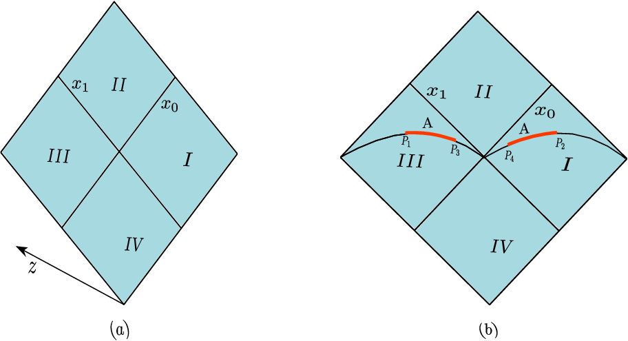
It is now useful to describe the different regions of the BTZ black string and relate each coordinate patch to the Poincaré coordinates,

$$ds^{2}=\frac{1}{z^{2}}(-dx_{0}^{2}+dx_{1}^{2}+dz^{2}).$$

(26)

The exterior metric of the BTZ black string is given as

$$ds^{2}=-\sinh^{2}\rho dt^{2}+\cosh^{2}\rho dx^{2}+d\rho^{2},$$

(27)

where the horizon is located at $\rho=0$, and the boundary is at $\rho\rightarrow\infty$. The BTZ coordinates $(t,x,\rho)$ covers a part of the Poincaré patch, close to the boundary and are related to the Poincaré coordinates as follows

$$x_{1}\pm x_{0}\approx e^{-x\pm t}\ ,\quad\quad{1\over z}\approx{1\over 2}e^{\rho-x}.$$

(28)

The coordinates $(t,x)$ cover the Rindler wedge denoted as the region $I$ of the Minkowski diamond in Fig. 3(a). It is possible to reach the other Rindler wedge denoted by the region $III$ in Fig. 3(a) by analytically continuing the time $t\to t+i\pi$. This is the continuation through which it is possible to reach from one side of the exterior region of the black string Penrose diagram to the other. The interior metric to the horizon $\rho=0$ is obtained by analytically continuing the coordinates $\rho=i\alpha,t=\tilde{t}-i\pi/2$ in eq. (27) as follows

$$ds^{2}=\sin^{2}\alpha d\tilde{t}^{2}+\cos^{2}\alpha dx^{2}-d\alpha^{2}.$$

(29)

These coordinates cover some part of the interior region and meet the boundary along the light cone $x_{0}^{2}-x_{1}^{2}=0$ as depicted in Fig. 3(a). The corresponding future bulk region of the interior to the BTZ black string is obtained by setting $\alpha=\pi/2-i\tilde{\rho},x=\tilde{x}-i\pi/2$ in eq. (29), which is given as

$$ds^{2}=\cosh^{2}\tilde{\rho}d\tilde{t}^{2}-\sinh^{2}\tilde{\rho}d\tilde{x}^{2}+d\tilde{\rho}^{2}.$$

(30)

The boundary of this future region in the Poincaré coordinates is given as $z\leq x_{0}^{2}-x_{1}^{2}$.

We now consider the interval $A$ of length $\ell$ on both the Rindler wedges $I$ and $III$ of the Minkowski diamond in Fig. 3(b). These two intervals are described as $(P_{1},P_{3})$ and $(P_{2},P_{4})$ in the $x_{1}$-$z$ plane of the Poincaré coordinates as depicted in Fig. (4). The coordinates of the end points of the intervals at a time $t$ are given from eq. (28) as follows Hartman:2013qma

	$\displaystyle P_{1}=$	$\displaystyle(\sinh t,-\cosh t),~~~P_{3}=e^{-\ell}P_{1},$		(31)
	$\displaystyle P_{2}=$	$\displaystyle(\sinh t,\cosh t),~~~~~~P_{4}=e^{-\ell}P_{2}.$

At early time $t\leq\ell/2$, the entanglement entropy receives contribution form the lengths of the geodesics $\mathcal{L}_{12}$ and $\mathcal{L}_{34}$ between the points $P_{1}$ to $P_{3}$ and $P_{2}$ to $P_{4}$ respectively as depicted in Fig. 4. These geodesics pass through the interior region in eq. (29) of the BTZ black string connecting one Rindler wedge to the other (the dashed geodesics in Fig. 4). These two geodesics are semicircles and they have identical regularized lengths. The entanglement entropy at early time $t\leq\ell/2$ is then given as follows Hartman:2013qma

	$\displaystyle S_{A}^{(1)}=$	$\displaystyle\frac{1}{4G_{N}}(\mathcal{L}_{12}+\mathcal{L}_{34}),$		(32)
	$\displaystyle=$	$\displaystyle\frac{4\pi ct}{3\beta}+4S_{div}.$

Here $S_{div}=\frac{c}{6}\ln\left(\frac{\beta}{4\pi\epsilon}\right)$ is the divergent part of the entanglement entropy, $\beta=4\tau_{0}$ is the inverse temperature and $\epsilon$ is the UV cut off.

On the other hand for times $t>\ell/2$ the entanglement entropy receives contribution from the lengths of the geodesics $\mathcal{L}_{13}$ and $\mathcal{L}_{42}$ between the points $P_{1}$ to $P_{3}$ and $P_{2}$ to $P_{4}$ respectively. These geodesics are confined to the exterior region of the BTZ black string outside the horizon as described in eq. (27) (depicted by the solid lines in the Fig. 4). The entanglement entropy for time $t>\ell/2$ is then given as

	$\displaystyle S_{A}^{(2)}=$	$\displaystyle\frac{1}{4G_{N}}(\mathcal{L}_{13}+\mathcal{L}_{24}),$		(33)
	$\displaystyle=$	$\displaystyle\frac{2\pi c\ell}{3\beta}+4S_{div}.$

It is observed from the above development that at early time the geodesics pass through the interior region of the BTZ black brane geometry from one Rindler wedge $I$ to the other $III$ and the linear increase of the holographic entanglement entropy is related to the growth of the nice slice in the interior. On the other hand for late times the geodesics are confined to the exterior region sitting outside the horizon and the corresponding entanglement entropy becomes thermal.

As mentioned earlier the bulk dual geometry corresponding to a global quench in a $CFT_{1+1}$ where the initial state is the conformal invariant boundary state $|B\rangle$ Calabrese:2005in is described by the eternal black hole sliced in half by an ETW brane (single sided black hole). Hence the corresponding holographic entanglement entropy for the interval $A$ in this case is then described by half of that obtained in eqs. (32) and (33) respectively. Remarkably, these results match exactly with the corresponding $CFT_{1+1}$ computation through the replica technique in eq. (7).

In this section we present our holographic construction for the time evolution of the entanglement negativity of two disjoint and adjacent intervals in a $CFT_{1+1}$ following a global quench as described in Coser:2014gsa. Motivated by the holographic construction for the time evolution of the entanglement entropy in Hartman:2013qma reviewed above, we begin by computing the holographic entanglement negativity for the mixed states under consideration from the bulk dual eternal black hole geometry. The corresponding holographic entanglement negativity following a global quench may then be obtained by considering half of the result for the bulk dual eternal black hole geometry.

It interesting to note that the four point twist correlator in eq. (12) admits a factorization with the non universal function ${\cal F}(\{\eta_{j,k}\})\to 1$ for the cross ratios $\eta_{i,j}\to 1$ and $\eta_{i,j}\to 0$, as follows

		$\displaystyle\langle\mathcal{T}_{n}(w_{1})\overline{\mathcal{T}}_{n}(w_{2})\overline{\mathcal{T}}_{n}(w_{3})\mathcal{T}_{n}(w_{4})\rangle_{\rm strip}=$		(34)
		$\displaystyle\frac{\langle\mathcal{T}_{n}(w_{1})\overline{\mathcal{T}}_{n}(w_{4})\rangle_{\rm strip}~\langle\mathcal{T}_{n}(w_{2})\overline{\mathcal{T}}_{n}(w_{3})\rangle_{\rm strip}~\Big(\langle\,\mathcal{T}^{2}_{n}(w_{1})\bar{\mathcal{T}}^{2}_{n}(w_{3})\,\rangle_{\rm strip}~\langle\,\mathcal{T}^{2}_{n}(w_{2})\bar{\mathcal{T}}^{2}_{n}(w_{4})\,\rangle_{\rm strip}\Big)^{\frac{1}{2}}}{\langle\mathcal{T}_{n}(w_{1})\overline{\mathcal{T}}_{n}(w_{3})\rangle_{\rm strip}~\langle\mathcal{T}_{n}(w_{2})\overline{\mathcal{T}}_{n}(w_{4})\rangle_{\rm strip}~\Big(\langle\,\mathcal{T}^{2}_{n}(w_{1})\bar{\mathcal{T}}^{2}_{n}(w_{4})\,\rangle_{\rm strip}~\langle\,\mathcal{T}^{2}_{n}(w_{2})\bar{\mathcal{T}}^{2}_{n}(w_{3})\,\rangle_{\rm strip}\Big)^{\frac{1}{2}}},$

where we have employed eq. (5) and the following two point twist correlator

$$\langle\mathcal{T}^{2}_{n}(w_{1})\bar{\mathcal{T}}^{2}_{n}(w_{2})\rangle_{\rm strip}=\left(\frac{\pi}{2\tau_{0}}\right)^{2\Delta^{(2)}_{n}}\frac{c^{(2)}_{n}}{|(z_{1}-\bar{z}_{1})(z_{2}-\bar{z}_{2})\,\eta_{1,2}|^{\Delta^{(2)}_{n}}}{\cal F}(\eta_{1,2})\,.$$

(35)

The entanglement negativity for two disjoint intervals may then be obtained by utilizing eqs. (11) and (34) which leads to following expression

$\displaystyle{\cal E}=$

$\displaystyle\frac{3}{4}\left(S_{A_{1}\cup A_{s}}+S_{A_{s}\cup A_{2}}-S_{A_{1}\cup A_{2}\cup A_{s}}-S_{A_{s}}\right),$

(36)

where $S_{\gamma}~(\gamma\in A_{1}\cup A_{s},~A_{s}\cup A_{2},~A_{1}\cup A_{2}\cup A_{s},~A_{s})$ is the entanglement entropy of an interval $\gamma$ as given in eq. (7).

Note that a similar factorization also holds for the three point twist correlator defined in eq. (20) which is given as

$\displaystyle\langle\mathcal{T}_{n}(w_{1})\bar{\mathcal{T}}^{2}_{n}(w_{2})\mathcal{T}_{n}(w_{3})\rangle_{\rm strip}\,=$

$\displaystyle\Bigg(\frac{\langle\,\mathcal{T}^{2}_{n}(w_{1})\bar{\mathcal{T}}^{2}_{n}(w_{2})\,\rangle_{\rm strip}~\langle\,\mathcal{T}^{2}_{n}(w_{2})\bar{\mathcal{T}}^{2}_{n}(w_{3})\,\rangle_{\rm strip}\langle\mathcal{T}_{n}(w_{1})\overline{\mathcal{T}}_{n}(w_{3})\rangle_{\rm strip}^{2}}{\langle\,\mathcal{T}^{2}_{n}(w_{1})\bar{\mathcal{T}}^{2}_{n}(w_{3})\,\rangle_{\rm strip}}\Bigg)^{1/2}.$

(37)

The entanglement negativity for two adjacent intervals may then be obtained by utilizing eqs. (11) and (37) as follows

$$\mathcal{E}=\frac{3}{4}(S_{A_{1}}+S_{A_{2}}-S_{A_{1}\cup A_{2}}).$$

(38)

In what follows we utilize eqs. (36) and (38) to establish the holographic entanglement negativity and its time evolution for two disjoint and adjacent intervals in a $CFT_{1+1}$ after a global quench employing the prescription for the holographic entanglement entropy described in Hartman:2013qma.

References

- (1) P. Calabrese and J. L. Cardy, Entanglement entropy and quantum field theory, J. Stat. Mech. 0406 (2004) P06002, [hep-th/0405152].
- (2) P. Calabrese and J. Cardy, Entanglement entropy and conformal field theory, J. Phys. A42 (2009) 504005, [0905.4013].
- (3) G. Vidal and R. F. Werner, Computable measure of entanglement, Phys. Rev. A 65 (Feb, 2002) 032314.
- (4) M. B. Plenio, Logarithmic Negativity: A Full Entanglement Monotone That is not Convex, Phys. Rev. Lett. 95 (2005) 090503, [quant-ph/0505071].
- (5) P. Calabrese, J. Cardy and E. Tonni, Entanglement negativity in quantum field theory, Phys. Rev. Lett. 109 (2012) 130502, [1206.3092].
- (6) P. Calabrese, J. Cardy and E. Tonni, Entanglement negativity in extended systems: A field theoretical approach, J. Stat. Mech. 1302 (2013) P02008, [1210.5359].
- (7) P. Calabrese, J. Cardy and E. Tonni, Finite temperature entanglement negativity in conformal field theory, J. Phys. A48 (2015) 015006, [1408.3043].
- (8) S. Ryu and T. Takayanagi, Holographic derivation of entanglement entropy from AdS/CFT, Phys. Rev. Lett. 96 (2006) 181602, [hep-th/0603001].
- (9) S. Ryu and T. Takayanagi, Aspects of Holographic Entanglement Entropy, JHEP 08 (2006) 045, [hep-th/0605073].
- (10) T. Takayanagi, Entanglement Entropy from a Holographic Viewpoint, Class. Quant. Grav. 29 (2012) 153001, [1204.2450].
- (11) T. Nishioka, S. Ryu and T. Takayanagi, Holographic Entanglement Entropy: An Overview, J. Phys. A42 (2009) 504008, [0905.0932].
- (12) T. Nishioka, Entanglement entropy: holography and renormalization group, 1801.10352.
- (13) M. Cadoni and M. Melis, Entanglement entropy of ads black holes, Entropy 12 (2010) 2244–2267.
- (14) D. D. Blanco, H. Casini, L.-Y. Hung and R. C. Myers, Relative Entropy and Holography, JHEP 08 (2013) 060, [1305.3182].
- (15) W. Fischler and S. Kundu, Strongly coupled gauge theories: high and low temperature behavior of non-local observables, Journal of High Energy Physics 2013 (May, 2013) 98.
- (16) W. Fischler, A. Kundu and S. Kundu, Holographic Mutual Information at Finite Temperature, Phys. Rev. D87 (2013) 126012, [1212.4764].
- (17) P. Chaturvedi, V. Malvimat and G. Sengupta, Entanglement thermodynamics for charged black holes, Phys. Rev. D94 (2016) 066004, [1601.00303].
- (18) D. V. Fursaev, Proof of the holographic formula for entanglement entropy, JHEP 09 (2006) 018, [hep-th/0606184].
- (19) M. Headrick, Entanglement Renyi entropies in holographic theories, Phys. Rev. D82 (2010) 126010, [1006.0047].
- (20) T. Faulkner, The Entanglement Renyi Entropies of Disjoint Intervals in AdS/CFT, 1303.7221.
- (21) H. Casini, M. Huerta and R. C. Myers, Towards a derivation of holographic entanglement entropy, JHEP 05 (2011) 036, [1102.0440].
- (22) A. Lewkowycz and J. Maldacena, Generalized gravitational entropy, JHEP 08 (2013) 090, [1304.4926].
- (23) V. E. Hubeny, M. Rangamani and T. Takayanagi, A Covariant holographic entanglement entropy proposal, JHEP 07 (2007) 062, [0705.0016].
- (24) X. Dong, A. Lewkowycz and M. Rangamani, Deriving covariant holographic entanglement, JHEP 11 (2016) 028, [1607.07506].
- (25) M. Rangamani and M. Rota, Comments on Entanglement Negativity in Holographic Field Theories, JHEP 10 (2014) 060, [1406.6989].
- (26) E. Perlmutter, M. Rangamani and M. Rota, Central Charges and the Sign of Entanglement in 4D Conformal Field Theories, Phys. Rev. Lett. 115 (2015) 171601, [1506.01679].
- (27) P. Chaturvedi, V. Malvimat and G. Sengupta, Holographic Quantum Entanglement Negativity, JHEP 05 (2018) 172, [1609.06609].
- (28) P. Chaturvedi, V. Malvimat and G. Sengupta, Covariant holographic entanglement negativity, Eur. Phys. J. C78 (2018) 776, [1611.00593].
- (29) V. Malvimat and G. Sengupta, Entanglement negativity at large central charge, 1712.02288.
- (30) P. Chaturvedi, V. Malvimat and G. Sengupta, Entanglement negativity, Holography and Black holes, Eur. Phys. J. C78 (2018) 499, [1602.01147].
- (31) P. Jain, V. Malvimat, S. Mondal and G. Sengupta, Holographic entanglement negativity conjecture for adjacent intervals in , 1707.08293.
- (32) P. Jain, V. Malvimat, S. Mondal and G. Sengupta, Covariant Holographic Entanglement Negativity Conjecture for Adjacent Subsystems in , 1710.06138.
- (33) P. Jain, V. Malvimat, S. Mondal and G. Sengupta, Holographic entanglement negativity for adjacent subsystems in AdSd+1/CFTd, Eur. Phys. J. Plus 133 (2018) 300, [1708.00612].
- (34) P. Jain, V. Malvimat, S. Mondal and G. Sengupta, Holographic Entanglement Negativity for Conformal Field Theories with a Conserved Charge, Eur. Phys. J. C78 (2018) 908, [1804.09078].
- (35) V. Malvimat, S. Mondal, B. Paul and G. Sengupta, Holographic entanglement negativity for disjoint intervals in , 1810.08015.
- (36) V. Malvimat, S. Mondal, B. Paul and G. Sengupta, Covariant holographic entanglement negativity for disjoint intervals in , 1812.03117.
- (37) P. Calabrese and J. L. Cardy, Evolution of entanglement entropy in one-dimensional systems, J. Stat. Mech. 0504 (2005) P04010, [cond-mat/0503393].
- (38) P. Calabrese and J. Cardy, Quantum quenches in 1+ 1 dimensional conformal field theories, Journal of Statistical Mechanics: Theory and Experiment 2016 (2016) 064003, [1603.02889].
- (39) X. Wen, S. Ryu and A. W. W. Ludwig, Entanglement hamiltonian evolution during thermalization in conformal field theory, 1807.04440.
- (40) X. Wen, P.-Y. Chang and S. Ryu, Entanglement negativity after a local quantum quench in conformal field theories, Phys. Rev. B92 (2015) 075109, [1501.00568].
- (41) A. Coser, E. Tonni and P. Calabrese, Entanglement negativity after a global quantum quench, J. Stat. Mech. 1412 (2014) P12017, [1410.0900].
- (42) M. Fagotti and P. Calabrese, Evolution of entanglement entropy following a quantum quench: Analytic results for the chain in a transverse magnetic field, Phys. Rev. A 78 (Jul, 2008) 010306.
- (43) P. Calabrese, F. H. L. Essler and M. Fagotti, Quantum quench in the transverse-field ising chain, Phys. Rev. Lett. 106 (Jun, 2011) 227203.
- (44) P. Calabrese and J. Cardy, Quantum Quenches in Extended Systems, J. Stat. Mech. 0706 (2007) P06008, [0704.1880].
- (45) P. Calabrese and J. L. Cardy, Time-dependence of correlation functions following a quantum quench, Phys. Rev. Lett. 96 (2006) 136801, [cond-mat/0601225].
- (46) J. Abajo-Arrastia, J. Aparicio and E. Lopez, Holographic Evolution of Entanglement Entropy, JHEP 11 (2010) 149, [1006.4090].
- (47) J. Aparicio and E. Lopez, Evolution of Two-Point Functions from Holography, JHEP 12 (2011) 082, [1109.3571].
- (48) T. Albash and C. V. Johnson, Evolution of Holographic Entanglement Entropy after Thermal and Electromagnetic Quenches, New J. Phys. 13 (2011) 045017, [1008.3027].
- (49) V. Balasubramanian, A. Bernamonti, J. de Boer, N. Copland, B. Craps, E. Keski-Vakkuri et al., Thermalization of Strongly Coupled Field Theories, Phys. Rev. Lett. 106 (2011) 191601, [1012.4753].
- (50) V. Balasubramanian, A. Bernamonti, J. de Boer, N. Copland, B. Craps, E. Keski-Vakkuri et al., Holographic Thermalization, Phys. Rev. D84 (2011) 026010, [1103.2683].
- (51) A. Allais and E. Tonni, Holographic evolution of the mutual information, JHEP 01 (2012) 102, [1110.1607].
- (52) H. Liu and S. J. Suh, Entanglement Tsunami: Universal Scaling in Holographic Thermalization, Phys. Rev. Lett. 112 (2014) 011601, [1305.7244].
- (53) H. Liu and S. J. Suh, Entanglement growth during thermalization in holographic systems, Phys. Rev. D89 (2014) 066012, [1311.1200].
- (54) T. Ugajin, Two dimensional quantum quenches and holography, 1311.2562.
- (55) H. Liu and J. Sonner, Holographic systems far from equilibrium: a review, 1810.02367.
- (56) T. Anous, T. Hartman, A. Rovai and J. Sonner, From Conformal Blocks to Path Integrals in the Vaidya Geometry, JHEP 09 (2017) 009, [1706.02668].
- (57) T. Hartman and J. Maldacena, Time Evolution of Entanglement Entropy from Black Hole Interiors, JHEP 05 (2013) 014, [1303.1080].
- (58) S. Cooper, M. Rozali, B. Swingle, M. Van Raamsdonk, C. Waddell and D. Wakeham, Black Hole Microstate Cosmology, 1810.10601.
- (59) W. Israel, Thermo field dynamics of black holes, Phys. Lett. A57 (1976) 107–110.
- (60) J. M. Maldacena, Eternal black holes in anti-de Sitter, JHEP 04 (2003) 021, [hep-th/0106112].
- (61) J. Polchinski, String theory and black hole complementarity, in Future perspectives in string theory. Proceedings, Conference, Strings’95, Los Angeles, USA, March 13-18, 1995, pp. 417–426, 1995, hep-th/9507094.
- (62) A. Buchel, L. Lehner, R. C. Myers and A. van Niekerk, Quantum quenches of holographic plasmas, JHEP 05 (2013) 067, [1302.2924].
- (63) T. Hartman, Entanglement Entropy at Large Central Charge, 1303.6955.
- (64) J. M. Maldacena and A. Strominger, AdS(3) black holes and a stringy exclusion principle, JHEP 12 (1998) 005, [hep-th/9804085].