跳到论文正文
W Papers独立论文阅读器 arXiv:1812.04356 论文正文 计算阅读时间 · 0%
引用这篇论文根据当前论文元数据生成,正式投稿前建议核对。


License: arXiv.org perpetual non-exclusive license
arXiv:1812.04356v3 [math.ST] 09 Sep 2020

Robust Bregman Clustering

Brécheteau    Claire Email: claire.brecheteau@univ-rennes2.fr Affiliation: Université Rennes 2 – IRMAR    Fischer    Aurélie Email: aurelie.fischer@lpsm.paris Affiliation: Université de Paris – LPSM    Levrard    Clément Email: clement.levrard@lpsm.paris Affiliation: Université de Paris – LPSM
Abstract

Clustering with Bregman divergences encompasses a wide family of clustering procedures that are well-suited to mixtures of distributions from exponential families [3]. However these techniques are highly sensitive to noise. To address the issue of clustering data with possibly adversarial noise, we introduce a robustified version of Bregman clustering based on a trimming approach. We investigate its theoretical properties, showing for instance that our estimator converges at a sub-Gaussian rate 1/n1/\sqrt{n}, where nn denotes the sample size, under mild tail assumptions. We also show that it is robust to a certain amount of noise, stated in terms of Breakdown Point. We also derive a Lloyd-type algorithm with a trimming parameter, along with a heuristic to select this parameter and the number of clusters from sample. Some numerical experiments assess the performance of our method on simulated and real datasets.

1 Introduction

Clustering is the problem of classifying data in groups of similar points, so that the groups are as homogeneous and at the same time as well separated as possible [18]. There are no labels known in advance, so clustering is an unsupervised learning task. To perform clustering, a distance-like function d⁡(⋅,⋅)d(\cdot,\cdot) is often needed to assess a notion of proximity between points and the separation between clusters.

Suppose that we know such a natural distance dd, and assume that the points we want to cluster, say X1,…,XnX_{1},\dots,X_{n}, are i.i.d., drawn from an unknown distribution PP, and take values in ℝd\mathbb{R}^{d}. For k≥1k\geq 1, designing kk meaningful classes with respect to dd can be achieved via minimizing the so-called empirical distortion

Rn​(𝐜)=1n​∑i=1nminj∈[[1,k]]⁡d⁡(Xi,cj),R_{n}(\mathbf{c})=\frac{1}{n}\sum_{i=1}^{n}\min_{j\in[\![1,k]\!]}d(X_{i},c_{j}),

over all possible cluster centers or codebooks 𝐜=(c1,…,ck)\mathbf{c}=(c_{1},\dots,c_{k}), with notation [[1,k]][\![1,k]\!] for {1,2,…,k}\{1,2,\dots,k\}. This results in a set of kk codepoints. Clusters are then given by the sets of sample points that have the same closest codepoint.

A classical choice of dd is the squared Euclidean distance, leading to the standard kk-means clustering algorithm (see, e.g., [31]). However, some of the desirable properties of the Euclidean distance can be extended to a broader class of dissimilarity functions, namely Bregman divergences. These distance-like functions, denoted by dϕd_{\phi} in the sequel, are indexed by strictly convex functions ϕ\phi. Introduced by [7], they are useful in a wide range of areas, among which statistical learning and data mining ([3], [11]), computational geometry [34], natural sciences, speech processing and information theory [24]. Squared Euclidean, Mahalanobis, Kullback-Leibler and L2L^{2} distances are all particular cases of Bregman divergences.

A Bregman divergence is not necessarily a true metric, since it may be asymmetric or fail to satisfy the triangle inequality. However, Bregman divergences fulfill an interesting projection property which generalizes the Hilbert projection on a closed convex set [7]. They also satisfy non-negativity and separation, convexity in the first argument and linearity (see [3], [34]). Moreover, Bregman divergences are closely related to exponential families [3]. In fact, they are a natural tool to measure proximity between observations arising from a mixture of such distributions. Consequently, clustering with Bregman divergences is particularly well-suited in this case.

Clustering with Bregman divergences allows to state the clustering problem within a contrast minimization framework. Namely, through minimizing Rn​(𝐜)=Pn​dϕ​(u,𝐜)R_{n}(\mathbf{c})=P_{n}d_{\phi}(u,\mathbf{c}), where PnP_{n} denotes the empirical distribution associated with {X1,…,Xn}\{X_{1},\dots,X_{n}\} and Q​f​(u)Qf(u) means integration of ff with respect to the measure QQ, we intend to find a codebook 𝐜^n\hat{\mathbf{c}}_{n} whose “real” distortion P​dϕ​(u,𝐜^n)Pd_{\phi}(u,\hat{\mathbf{c}}_{n}) is close to the optimal kk-points distortion Rk∗:=inf𝐜P​dϕ​(u,𝐜)R^{*}_{k}:=\inf_{\mathbf{c}}Pd_{\phi}(u,\mathbf{c}). The convergence properties of empirical distortion minimizers are now quite well understood when the source distribution PP is assumed to have a finite support [30, 21], even in infinite-dimensional cases [4, 28]. In real data sets, the source signal is often corrupted by noise, violating in most cases the bounded support assumption. In practice, data are usually pre-processed via an outlier-removal step that requires an important quantity of expertise. From a theoretical viewpoint, this corruption issue might be tackled by winsorizing or trimming classical estimators, or by introducing some new and robust estimators that adapt to heavy-tailed cases. Such estimators can be based on PAC-Bayesian or Median of Means techniques [10, 8, 27] for instance. In a nutshell, these estimators succeed in achieving sub-Gaussian deviation bounds under mild tail conditions such as bounded variances and expectations, and they are also provably robust to a certain amount of noise [27].

In the clustering framework, it is straightforward that the kk-means procedure suffers from the same drawback as the empirical mean: only one adversarial datapoint is needed to drive both the empirically optimal codebook 𝐜^n\hat{\mathbf{c}}_{n} and its distortion arbitrarily far from the optimal. In fact we show that it is the case with every possible Bregman divergence. Up to our knowledge, the only theoretically grounded attempt to robustify clustering procedures is to be found in [16], where a trimmed kk-means heuristic is introduced. See also [19] for trimmed clustering with Mahalanobis distances. In some sense, this paper extends this trimming approach to the general framework of clustering with Bregman divergences.

We introduce some notation, background and fundamental properties for trimmed clustering with Bregman divergences in Section 2. This will lead to the description of our robust clustering technique, based on the computation of a trimmed empirically optimal codebook 𝐜^n,h\hat{\mathbf{c}}_{n,h}, for a fixed trim level hh.

Theoretical properties of our trimmed empirical codebook 𝐜^n,h\hat{\mathbf{c}}_{n,h} are exposed in Section 3. To be more precise, we investigate convergence towards a trimmed optimal codebook 𝐜h∗\mathbf{c}^{*}_{h} in terms of distance and distortion, showing for instance that the excess distortion achieves a sub-Gaussian convergence rate of O⁡(1/n)O(1/\sqrt{n}) in terms of sample size, under a mild bounded variance assumption. This shows that our procedure can be thought of as robust whenever noisy situations are modeled as a signal corrupted with heavy-tailed additive noise. We also assess robustness of 𝐜^n,h\hat{\mathbf{c}}_{n,h} in terms of Finite-sample Breakdown Point (see, e.g., [32]), showing that our procedure can theoretically endure a positive proportion of adversarial noise. A precise bound on this proportion is given, that illustrates the possible confusion between too small clusters and noise.

Then, a modified Lloyd’s type algorithm is proposed in Section 4, along with a heuristic to select both the trim level hh and the number kk of clusters from data. The numerical performances of our algorithm are then investigated. We compare our method to trimmed kk-means [16], tclust [22], ToMATo [14], dbscan [25] and a trimmed version of kk-median [9]. Our algorithm with the appropriate Bregman divergence outperforms other methods on samples generated from Gaussian, Poisson, Binomial, Gamma and Cauchy mixtures. We then investigate the performances of our method on real datasets. First, we consider daily rainfall measurements for January and September in Cayenne, from 2007 to 2017, and try to cluster data according to the month. As suggested by [15], our method with the divergence associated with Gamma distributions turns out to be the most accurate one. Second, we intend to cluster chunks of 50005000 words picked from novels corresponding to 44 different authors, based on stylometric descriptors [38, Section 10], corrupted by noise. Following [20], we show that our method with Poisson divergence is particularly well adapted for this framework.

At last, proofs are gathered in Sections 5 and 6. Proofs of technical intermediate results are deferred to Sections 7, 8, 9, and 10, along with some additional figures and results for Section 4.

2 Clustering with trimmed Bregman divergence

2.1 Bregman divergences and distortion

A Bregman divergence is defined as follows.

Definition 1.

Let ϕ\phi be a strictly convex 𝒞1\mathcal{C}_{1} real-valued function defined on a convex set Ω⊂ℝd\Omega\subset\mathbb{R}^{d}. The Bregman divergence dϕd_{\phi} is defined for all x,y∈Ωx,y\in\Omega by

dϕ​(x,y)=ϕ⁡(x)−ϕ⁡(y)−⟨∇yϕ,x−y⟩.d_{\phi}(x,y)=\phi(x)-\phi(y)-\langle\nabla_{y}\phi,x-y\rangle.

Observe that, since ϕ\phi is strictly convex, for all x,y∈ℝdx,y\in\mathbb{R}^{d}, dϕ​(x,y)d_{\phi}(x,y) is non-negative and equal to zero if and only if x=yx=y (see [35, Theorem 25.1]). Note that by taking ϕ:x↦‖x‖2\phi:x\mapsto\|x\|^{2}, with ∥⋅∥\|\cdot\| the Euclidean norm on ℝd\mathbb{R}^{d}, one gets dϕ​(x,y)=‖x−y‖2d_{\phi}(x,y)=\|x-y\|^{2}. Let us present a few other examples:

  1. 1.

    Exponential loss: ϕ:x↦ex\phi:x\mapsto e^{x}, from ℝ\mathbb{R} to ℝ\mathbb{R}, leads to dϕ​(x,y)=ex−ey−(x−y)​eyd_{\phi}(x,y)=e^{x}-e^{y}-(x-y)e^{y}.

  2. 2.

    Logistic loss: ϕ:x↦x​ln⁡x+(1−x)​ln⁡(1−x)\phi:x\mapsto x\ln x+(1-x)\ln(1-x), from [0,1][0,1] to ℝ\mathbb{R}, leads to dϕ​(x,y)=x​ln⁡xy+(1−x)​ln⁡(1−x1−y)d_{\phi}(x,y)=x\ln\frac{x}{y}+(1-x)\ln\big(\frac{1-x}{1-y}\big).

  3. 3.

    Kullback-Leibler: ϕ:x↦∑ℓ=1dxℓ​ln⁡xℓ\phi:x\mapsto\sum_{\ell=1}^{d}x_{\ell}\ln x_{\ell}, from the (d−1)−(d-1)-simplex to ℝ\mathbb{R}, leads to dϕ​(x,y)=∑ℓ=1dxℓ​ln⁡xℓyℓd_{\phi}(x,y)=\sum_{\ell=1}^{d}x_{\ell}\ln\frac{x_{\ell}}{y_{\ell}}.

For any compact set K⊂ΩK\subset\Omega, and x∈Ωx\in\Omega, we also define

dϕ​(K,x)=miny∈K⁡dϕ​(y,x)anddϕ​(x,K)=miny∈K⁡dϕ​(x,y).\displaystyle d_{\phi}(K,x)=\min_{y\in K}d_{\phi}(y,x)\quad\mbox{and}\quad d_{\phi}(x,K)=\min_{y\in K}d_{\phi}(x,y).

For every codebook 𝐜=(c1,c2,…,ck)∈Ω(k)\mathbf{c}=(c_{1},c_{2},\dots,c_{k})\in\Omega^{(k)}, dϕ​(x,𝐜)d_{\phi}(x,\mathbf{c}) is defined by dϕ​(x,𝐜)=mini∈[[1,k]]⁡dϕ​(x,ci)d_{\phi}(x,\mathbf{c})=\min_{i\in[\![1,k]\!]}d_{\phi}(x,c_{i}). The main property of Bregman divergences is that means are always minimizers of Bregman inertias, as exposed below. For a distribution QQ and a function ff, we denote by Q​f​(u)Qf(u) the integration of ff with respect to QQ.

Proposition 2.

[2, Theorem 1] Let PP be a probability distribution, and let ϕ\phi be a strictly convex 𝒞1\mathcal{C}_{1} real-valued function defined on a convex set Ω⊂ℝd\Omega\subset\mathbb{R}^{d}. Then, for any xx ∈\in Ω\Omega,

P​dϕ​(u,x)=P​dϕ​(u,P​u)+dϕ​(P​u,x).Pd_{\phi}(u,x)=Pd_{\phi}(u,Pu)+d_{\phi}(Pu,x).

As mentioned in [3], this property allows to design iterative Bregman clustering algorithms that are similar to Lloyd’s algorithm. Let PP be a distribution on ℝd\mathbb{R}^{d}, and 𝐜\mathbf{c} a codebook. The clustering performance of 𝐜\mathbf{c} will be measured via its distortion, namely

R⁡(𝐜)=P​dϕ​(u,𝐜).\displaystyle R(\mathbf{c})=Pd_{\phi}(u,\mathbf{c}).

When only an i.i.d. sample 𝕏n={X1,…,Xn}\mathbbm{X}_{n}=\{X_{1},\dots,X_{n}\} is available, we denote by Rn​(𝐜)R_{n}(\mathbf{c}) the corresponding empirical distortion (associated with PnP_{n}). When PP is a mixture of distributions belonging to an exponential family, there exists a natural choice of Bregman divergence, as detailed in Section 4. Standard Bregman clustering intends to infer a minimizer of RR via minimizing RnR_{n}, and works well in the bounded support case [21].

2.2 Trimmed optimal codebooks

As for classical mean estimation, plain kk-means is sensitive to outliers. An attempt to address this issue is proposed in [16, 23]: for a trim level h∈(0,1]h\in(0,1], both a codebook and a subset of PP-mass not smaller than hh (trimming set) are pursued. This heuristic can be generalized to our framework as follows.

For a measure QQ on ℝd\mathbb{R}^{d}, we write Q≪PQ\ll P (i.e., QQ is a sub-measure of PP) if Q⁡(A)≤P⁡(A)Q(A)\leq P(A) for every Borel set AA. Let 𝒫h\mathcal{P}_{h} denote the set 𝒫h={1hQ∣Q≪P,Q(ℝd)=h}\mathcal{P}_{h}=\{\frac{1}{h}Q\mid Q\ll P,Q(\mathbb{R}^{d})=h\}, and 𝒫+h=∪s≥h𝒫s\mathcal{P}_{+h}=\cup_{s\geq h}\mathcal{P}_{s}. By analogy with [16], optimal trimming sets and codebooks are designed to achieve the optimal hh-trimmed kk-variation,

Vk,h:=infP~∈𝒫+hinf𝐜∈Ω(k)R⁡(P~,𝐜),\displaystyle V_{k,h}:=\inf_{\tilde{P}\in\mathcal{P}_{+h}}\inf_{\mathbf{c}\in\Omega^{(k)}}R(\tilde{P},\mathbf{c}),

where R⁡(P~,𝐜)=P~​dϕ​(u,𝐜)R(\tilde{P},\mathbf{c})=\tilde{P}d_{\phi}(u,\mathbf{c}). In other words, Vk,hV_{k,h} is the best possible kk-point distortion based on a normalized sub-measure of PP. Intuitively speaking, the hh-trimmed kk-variation may be thought of as the kk-points optimal distortion of the best "denoised" version of PP, with denoising level 1−h1-h. For instance, in a mixture setting, if P=γ​P0+(1−γ)​NP=\gamma P_{0}+(1-\gamma)N, where P0P_{0} is a signal supported by kk points and NN is a noise distribution, then, provided that h≤γh\leq\gamma, Vk,h=0V_{k,h}=0.

If 𝐜\mathbf{c} is a fixed codebook, we denote by Bϕ​(𝐜,r)B_{\phi}(\mathbf{c},r) (resp B¯ϕ​(𝐜,r)\bar{B}_{\phi}(\mathbf{c},r)) the open (resp. closed) Bregman ball with radius rr, {x∣dϕ​(x,𝐜)<r}\left\{x\mid\sqrt{d_{\phi}(x,\mathbf{c})}<r\right\} (resp. ≤\leq), and by rh​(𝐜)r_{h}(\mathbf{c}) the smallest radius r≥0r\geq 0 such that

P⁡(Bϕ​(𝐜,r))≤h≤P⁡(B¯ϕ​(𝐜,r)).\displaystyle P(B_{\phi}(\mathbf{c},r))\leq h\leq P(\bar{B}_{\phi}(\mathbf{c},r)). (1)

We denote this radius by rn,h​(𝐜)r_{n,h}(\mathbf{c}) when the distribution is PnP_{n}. Note that rn,h​(𝐜)2r_{n,h}(\mathbf{c})^{2} is the Bregman divergence to the ⌈n​h⌉\lceil nh\rceil dϕd_{\phi}-nearest-neighbor of 𝐜\mathbf{c} in 𝕏n\mathbbm{X}_{n}. Now, if 𝒫h​(𝐜)\mathcal{P}_{h}(\mathbf{c}) is defined as the set of measures P~\tilde{P} in 𝒫h\mathcal{P}_{h} that coincide with Ph\frac{P}{h} on Bϕ​(𝐜,rh​(𝐜))B_{\phi}(\mathbf{c},r_{h}(\mathbf{c})), with support included in B¯ϕ​(𝐜,rh​(𝐜))\bar{B}_{\phi}(\mathbf{c},r_{h}(\mathbf{c})), a straightforward result is the following.

Lemma 3.

For all 𝐜∈Ω(k)\mathbf{c}\in\Omega^{(k)}, h∈(0,1]h\in(0,1], P~∈𝒫h\tilde{P}\in\mathcal{P}_{h} and P~𝐜∈𝒫h​(𝐜)\tilde{P}_{\mathbf{c}}\in\mathcal{P}_{h}(\mathbf{c}),

R⁡(P~𝐜,𝐜)≤R⁡(P~,𝐜).R(\tilde{P}_{\mathbf{c}},\mathbf{c})\leq R(\tilde{P},\mathbf{c}).

Equality holds if and only if P~∈𝒫h​(𝐜)\tilde{P}\in\mathcal{P}_{h}(\mathbf{c}).

This lemma is a straightforward generalisation of results in [16, Lemma 2.1], [23] or [13]. A short proof is given in Section 7.1. As a consequence, for any codebook 𝐜∈Ω(k)\mathbf{c}\in\Omega^{(k)} we may restrict our attention to sub-measures in 𝒫h​(𝐜)\mathcal{P}_{h}(\mathbf{c}).

Definition 4.

For 𝐜∈Ω(k)\mathbf{c}\in\Omega^{(k)}, the hh-trimmed distortion of 𝐜\mathbf{c} is defined by

Rh​(𝐜)=h​R​(P~𝐜,𝐜),R_{h}(\mathbf{c})=hR(\tilde{P}_{\mathbf{c}},\mathbf{c}),

where P~𝐜∈𝒫h​(𝐜)\tilde{P}_{\mathbf{c}}\in\mathcal{P}_{h}(\mathbf{c}).

Note that since R⁡(P~𝐜,𝐜)R(\tilde{P}_{\mathbf{c}},\mathbf{c}) does not depend on the choice of P~𝐜\tilde{P}_{\mathbf{c}} whenever P~𝐜∈𝒫h​(𝐜)\tilde{P}_{\mathbf{c}}\in\mathcal{P}_{h}(\mathbf{c}), Rh​(𝐜)R_{h}(\mathbf{c}) is well-defined. As well, Rn,h​(𝐜)R_{n,h}(\mathbf{c}) will denote the trimmed distortion corresponding to the distribution PnP_{n}. Another simple property of sub-measures can be translated in terms of trimmed distortion.

Lemma 5.

Let 0<h<h′<10<h<h^{\prime}<1 and 𝐜∈Ω(k)\mathbf{c}\in\Omega^{(k)}. Then

Rh​(𝐜)/h≤Rh′​(𝐜)/h′.{R_{h}(\mathbf{c})}/{h}\leq{R_{h^{\prime}}(\mathbf{c})}/{h^{\prime}}.

Moreover, equality holds if and only if P⁡(Bϕ​(𝐜,rh′​(𝐜)))=0P(B_{\phi}(\mathbf{c},r_{h^{\prime}}(\mathbf{c})))=0.

As well, this lemma generalizes previous results in [16, 23]. A proof can be found in Section 5.2. Lemma 3 and Lemma 5 ensure that for a given 𝐜\mathbf{c}, optimal P~\tilde{P} in 𝒫+h\mathcal{P}_{+h} for R⁡(P~,𝐜)R(\tilde{P},\mathbf{c}) can be found in 𝒫h​(𝐜)\mathcal{P}_{h}(\mathbf{c}). Thus, the optimal hh-trimmed kk-variation may be achieved via minimizing the hh-trimmed distortion.

Proposition 6.

For every positive integer kk and 0<h<10<h<1,

h​Vk,h=inf𝐜∈Ω(k)Rh​(𝐜).hV_{k,h}=\inf_{\mathbf{c}\in\Omega^{(k)}}R_{h}(\mathbf{c}).

This proposition is an extension of [16, Proposition 2.3]. In other words, Proposition 6 assesses the equivalence between minimization of our robustified distortion RhR_{h}, and the original robust clustering criterion depicted in [16] (extended to Bregman divergences). Thus, a good codebook in terms of trimmed kk-variation can be found by minimizing RhR_{h}.

Definition 7.

An hh-trimmed kk-optimal codebook is any element 𝐜∗\mathbf{c}^{*} in arg⁡min𝐜∈Ω(k)​Rh​(𝐜)\arg\min_{\mathbf{c}\in\Omega^{(k)}}R_{h}(\mathbf{c}).

Under mild assumptions on PP and ϕ\phi, trimmed kk-optimal codebooks exist.

Theorem 8.

Let 0<h<10<h<1, assume that P​‖u‖<+∞P\|u\|<+\infty, ϕ\phi is 𝒞2\mathcal{C}^{2} and strictly convex and F0=c​o​n​v​(s​u​p​p​(P))¯⊂Ω̊F_{0}=\overline{conv(supp(P))}\subset\mathring{\Omega}, that is, the closure of the convex hull of the support of PP is a subset of the interior of Ω\Omega. Then, the set arg⁡min𝐜∈Ω(k)​Rh​(𝐜)\arg\min_{\mathbf{c}\in\Omega^{(k)}}R_{h}(\mathbf{c}) is not empty.

A proof of Theorem 8 is given in Section 5.3. Note that Theorem 8 only requires P​‖u‖<+∞P\|u\|<+\infty. This can be compared with the standard squared Euclidean distance case, where P​‖u‖2<+∞P\|u\|^{2}<+\infty is required for R:𝐜↦P​‖u−𝐜‖2R:\mathbf{c}\mapsto P\|u-\mathbf{c}\|^{2} to have minimizers. From now on we denote by 𝐜h∗\mathbf{c}^{*}_{h} a minimizer of RhR_{h}, and by 𝐜^n,h\hat{\mathbf{c}}_{n,h} a minimizer of the empirical trimmed distortion Rn,hR_{n,h}.

2.3 Bregman-Voronoi cells and centroid condition

Similarly to the Euclidean case, the clustering associated with a codebook 𝐜\mathbf{c} will be given by a tesselation of the ambient space. To be more precise, for 𝐜∈Ω(k)\mathbf{c}\in\Omega^{(k)} and i∈[[1,k]]i\in[\![1,k]\!], the Bregman-Voronoi cell associated with cic_{i} is Vi(𝐜)={x∣∀j≠idϕ(x,ci)≤dϕ(x,cj)}V_{i}(\mathbf{c})=\{x\mid\forall j\neq i\quad d_{\phi}(x,c_{i})\leq d_{\phi}(x,c_{j})\}. Some further results on the geometry of Bregman Voronoi cells might be found in [34]. Since the Vi​(𝐜)V_{i}(\mathbf{c})’s do not form a partition, Wi​(𝐜)W_{i}(\mathbf{c}) will denote a subset of Vi​(𝐜)V_{i}(\mathbf{c}) so that {W1​(𝐜),…,Wk​(𝐜)}\{W_{1}(\mathbf{c}),\dots,W_{k}(\mathbf{c})\} is a partition of ℝd\mathbb{R}^{d} (for instance break the ties of the ViV_{i}’s with respect to the lexicographic rule). Proposition 9 below extends the so-called centroid condition in the Euclidean case to our Bregman setting.

Proposition 9.

Let 𝐜∈Ω(k)\mathbf{c}\in\Omega^{(k)} and P~𝐜∈𝒫h​(𝐜)\tilde{P}_{\mathbf{c}}\in\mathcal{P}_{h}(\mathbf{c}). Assume that for all i∈[[1,k]]i\in[\![1,k]\!], P~𝐜​(Wi​(𝐜))>0\tilde{P}_{\mathbf{c}}(W_{i}(\mathbf{c}))>0, and denote by 𝐦\mathbf{m} the codebook of the local means of P~𝐜\tilde{P}_{\mathbf{c}}. In other words, mi=P~𝐜​(u​𝟙Wi​(𝐜)​(u))/P~𝐜​(Wi​(𝐜))m_{i}=\tilde{P}_{\mathbf{c}}(u\mathbbm{1}_{W_{i}(\mathbf{c})}(u))/\tilde{P}_{\mathbf{c}}(W_{i}(\mathbf{c})). Then

Rh​(𝐜)≥Rh​(𝐦),\displaystyle R_{h}(\mathbf{c})\geq R_{h}(\mathbf{m}),

with equality if and only if for all ii in [[1,k]][\![1,k]\!], ci=mic_{i}=m_{i}.

Proposition 9 is a straightforward consequence of Proposition 2, that emphasizes the key property that Bregman divergences are minimized by expectations (this is not the case for the L1L_{1} distance for instance). In addition, it can be proved that Bregman divergences are the only loss functions satisfying this property [2]. In line with [3] for the non-trimmed case, Proposition 9 provides an iterative scheme to minimize RhR_{h}, that is detailed in Section 4.

3 Theoretical results

3.1 Convergence of a trimmed empirical distortion minimizer

This section is devoted to investigate the convergence of a minimizer 𝐜^n,h\hat{\mathbf{c}}_{n,h} of the empirical trimmed distortion Rn,hR_{n,h}. Throughout this section ϕ\phi is assumed to be 𝒞2\mathcal{C}^{2}, and F0=c​o​n​v​(s​u​p​p​(P))¯⊂Ω̊F_{0}=\overline{conv(supp(P))}\subset\mathring{\Omega}. We begin with a generalization of [16, Theorem 3.4], assessing the almost sure convergence of optimal empirical trimmed codebooks.

Theorem 10.

Assume that PP is absolutely continuous with respect to the Lebesgue measure and satisfies P​‖u‖p<∞P\|u\|^{p}<\infty for some p>2p>2, then there exists 𝐜h∗\mathbf{c}^{*}_{h} an optimal codebook such that

limn→+∞Rn,h​(𝐜^n,h)=Rh​(𝐜h∗)​ a.e..\lim_{n\rightarrow+\infty}R_{n,h}(\hat{\mathbf{c}}_{n,h})=R_{h}(\mathbf{c}^{*}_{h})\text{ a.e.}.

Moreover, up to extracting a subsequence, we have

limn→+∞D⁡(𝐜^n,h,𝐜h∗)=0​ a.e.,\lim_{n\rightarrow+\infty}D(\hat{\mathbf{c}}_{n,h},\mathbf{c}^{*}_{h})=0\text{ a.e.},

where D⁡(𝐜,𝐜′)=minσ∈Σk⁡maxi∈[[1,k]]​|ci−cσ⁡(i)′|D(\mathbf{c},\mathbf{c}^{\prime})=\min_{\sigma\in\Sigma_{k}}\max_{i\in[\![1,k]\!]}|c_{i}-c^{\prime}_{\sigma(i)}| and Σk\Sigma_{k} denotes the set of all permutations of [[1,k]][\![1,k]\!]. At last, if 𝐜h∗\mathbf{c}^{*}_{h} is unique, then limn→+∞D⁡(𝐜^n,h,𝐜h∗)=0​ a.e.\lim_{n\rightarrow+\infty}D(\hat{\mathbf{c}}_{n,h},\mathbf{c}^{*}_{h})=0\text{ a.e.} (without taking a subsequence).

Note that, contrary to [16, Theorem 3.4], uniqueness of trimmed optimal codebooks is not required in Theorem 10. A proof is given in Section 6.2. Interestingly, slightly milder conditions are required for the trimmed distortion of 𝐜^n,h\hat{\mathbf{c}}_{n,h} to converge towards the optimal at a parametric rate.

Theorem 11.

Assume that P​‖u‖p<∞P\|u\|^{p}<\infty, where p≥2p\geq 2. Further, if Rk,h∗R^{*}_{k,h} denotes the hh-trimmed optimal distortion with kk points, assume that Rk−1,h∗−Rk,h∗>0R^{*}_{k-1,h}-R^{*}_{k,h}>0. Then, for nn large enough, with probability larger than 1−n−p2−2​e−x1-n^{-\frac{p}{2}}-2e^{-x}, we have

Rh​(𝐜^n,h)−Rh​(𝐜h∗)≤CPn​(1+x).\displaystyle R_{h}(\hat{\mathbf{c}}_{n,h})-R_{h}(\mathbf{c}^{*}_{h})\leq\frac{C_{P}}{\sqrt{n}}(1+\sqrt{x}).

The requirement Rk−1,h∗−Rk,h∗>0R^{*}_{k-1,h}-R^{*}_{k,h}>0 ensures that optimal codebooks will not have empty cells. Note that if Rk−1,h∗−Rk,h∗=0R^{*}_{k-1,h}-R^{*}_{k,h}=0, then there exists a subset AA of ℝd\mathbb{R}^{d} satisfying P⁡(A)≥hP(A)\geq h and such that the restriction of PP to AA is supported by at most k−1k-1 points, that allows optimal kk-points codebooks with at least one empty cell. It is worth mentioning that Theorem 11 does not require a unique trimmed optimal codebook, and only requires an order 22 moment condition for 𝐜^n,h\hat{\mathbf{c}}_{n,h} to achieve a sub-Gaussian rate in terms of trimmed distortion. This condition is in line with the order 22 moment condition required in [8] for a robustified estimator of 𝐜∗\mathbf{c}^{*} to achieve similar guarantees, as well as the finite-variance condition required in [10] in a mean estimation framework. A proof of Theorem 11 is given in Section 6.3. To derive results in expectation, a technical additional condition is needed.

Corollary 12.

Assume that there exists a non-decreasing convex function ψ\psi such that

supc∈B⁡(0,t)∩F0‖∇cϕ‖≤ψ⁡(t).\sup_{c\in B(0,t)\cap F_{0}}\|\nabla_{c}\phi\|\leq\psi(t).

Assume that P​‖u‖p<∞P\|u\|^{p}<\infty, with p≥2p\geq 2, and let q=p/(p−1)q=p/(p-1) be the harmonic conjugate of pp. If P​‖u‖q​ψq​(k​‖u‖h)<∞P\|u\|^{q}\psi^{q}\left(\frac{k\|u\|}{h}\right)<\infty, then

𝔼⁡(Rh​(𝐜^n,h)−Rh​(𝐜h∗))≤CPn.\displaystyle\mathbb{E}\left(R_{h}(\hat{\mathbf{c}}_{n,h})-R_{h}(\mathbf{c}^{*}_{h})\right)\leq\frac{C_{P}}{\sqrt{n}}.

A proof of Corollary 12 is given in Section 6.4. Note that such a function ψ\psi exists in most of the classical cases. The requirement P​‖u‖q​ψq​(k​‖u‖/h)P\|u\|^{q}\psi^{q}({k\|u\|}/{h}) roughly ensures that P​dϕq​(u,𝐜^n,h)Pd_{\phi}^{q}(u,\hat{\mathbf{c}}_{n,h}) remains bounded whenever the event described in Theorem 11 does not occur. The moment condition required by Corollary 12 might be quite stronger than the order 22 condition of Theorem 11, as illustrated below.

  1. 1.

    In the kk-means case ϕ⁡(x)=‖x‖2\phi(x)=\|x\|^{2} and Ω=ℝd\Omega=\mathbb{R}^{d}, we can choose ψ⁡(t)=2​t\psi(t)=2t. The condition of Corollary 12 is satisfied for P​‖u‖3<+∞P\|u\|^{3}<+\infty.

  2. 2.

    For ϕ⁡(x)=exp⁡(x)\phi(x)=\exp(x), Ω=ℝ\Omega=\mathbb{R}, we may choose ψ⁡(t)=exp⁡(t)\psi(t)=\exp(t). The condition of Corollary 12 may be written for p=2p=2 as P​u2​exp⁡(2​k​|u|h)<+∞Pu^{2}\exp\left(\frac{2k|u|}{h}\right)<+\infty.

3.2 Robustness properties of trimmed empirical distortion minimizers

This section is devoted to discuss to what extent the trimming procedure we propose implies robustness of our estimator to adversarial contamination. First we choose to assess robustness via the so-called Finite-sample Breakdown Point [17], that seizes what proportion of adversarial noise can be added to a dataset without making estimators getting arbitrarily large. To be more precise, for an amount ss of adversarial points {x1,…,xs}\{x_{1},\dots,x_{s}\}, we denote by Pn+sP_{n+s} the empirical distribution associated with 𝕏n∪{x1,…,xs}\mathbbm{X}_{n}\cup\{x_{1},\dots,x_{s}\} and by 𝐜^n+s,h\hat{\mathbf{c}}_{n+s,h} a minimizer of 𝐜↦Rn+s,h​(𝐜)\mathbf{c}\mapsto{R}_{n+s,h}(\mathbf{c}). We may then define the Finite-sample Breakdown Point (FSBP) as follows:

B​P^n,h:=inf{sn+s∣sup{x1,…,xs}‖𝐜^n+s,h‖=+∞}.\displaystyle\widehat{BP}_{n,h}:=\inf\left\{\frac{s}{n+s}\mid\sup_{\{x_{1},\dots,x_{s}\}}\|\hat{\mathbf{c}}_{n+s,h}\|=+\infty\right\}.

To give an intuition, the standard mean (minimizer of the 11-trimmed empirical distortion for k=1k=1, ϕ⁡(u)=‖u‖2\phi(u)=\|u\|^{2}) has breakdown point 1n+1\frac{1}{n+1}, whereas hh-trimmed means have breakdown point roughly 1−h1-h (see, e.g., [32, Section 3.2.5]). According to [40, Theorem 1], this is also the case whenever ϕ\phi is strictly convex (but still k=1k=1). In the case k>1k>1, as noticed in [16] for trimmed kk-means, the breakdown point may be much smaller than 1−h1-h. Note that if an hh-trimmed optimal codebook has a too small cluster, then adding an adversarial cluster with greater weight might switch the roles between noise and signal, resulting in an hh-trimmed codebook that allocates one point to the adversarial cluster and trims the too small optimal cluster. To quantify this intuition, we introduce the following discernability factor BhB_{h}.

Definition 13.

Let h∈]0,1[h\in]0,1[, and, for b≤hb\leq h, denote by hb−=(h−b)/(1−b)h_{b}^{-}=(h-b)/(1-b), hb+=h/(1−b)h_{b}^{+}=h/(1-b). The discernability factor BhB_{h} is defined as

Bh=sup{b≥0∣b≤h∧(1−h)​ and ​minj∈[[2,k]]​Rj−1,hb−∗−Rj,hb+∗>0}.B_{h}=\sup\left\{b\geq 0\mid b\leq h\wedge(1-h)\text{ and }\min_{j\in[\![2,k]\!]}R^{*}_{j-1,h_{b}^{-}}-R^{*}_{j,h_{b}^{+}}>0\right\}.

In fact, h−hBh−=(1−h)​Bh/(1−Bh)h-h_{B_{h}}^{-}=(1-h)B_{h}/(1-B_{h}) is the portion of mass in an optimal kk-points hh trimming set that may be considered as noise by an optimal k−1k-1-points hBh−h_{B_{h}}^{-} trimming set. As exposed in the following proposition, BhB_{h} is related to the minimum cluster weight of optimal hh-trimmed codebooks.

Proposition 14.

Assume that the requirements of Theorem 8 are satisfied. If Rk−1,h∗−Rk,h∗>0R^{*}_{k-1,h}-R^{*}_{k,h}>0, then Bh>0B_{h}>0.

Moreover, for any j∈[[1,k]]j\in[\![1,k]\!], if 𝐜∗,(j)\mathbf{c}^{*,(j)} is a jj-points hh-trimmed optimal codebook and pj,h=h​minp∈[[1,j]]​P~𝐜∗,(j)​(Wp​(𝐜∗,(j)))p_{j,h}=h\min_{p\in[\![1,j]\!]}\tilde{P}_{\mathbf{c}^{*,(j)}}\left(W_{p}(\mathbf{c}^{*,(j)})\right), with P~𝐜∗,(j)∈𝒫h​(𝐜∗,(j))\tilde{P}_{\mathbf{c}^{*,(j)}}\in\mathcal{P}_{h}(\mathbf{c}^{*,(j)}), then

Bh​(1−(h−pj,h))≤pj,h.B_{h}(1-(h-p_{j,h}))\leq p_{j,h}.

A proof of Proposition 14 is given in Section 5.4. Theorem 15 below makes connection between this discernability factor and robustness properties of optimal kk-points hh-trimmed codebook, stated in terms of Bregman radius.

Theorem 15.

For ℓ≥1\ell\geq 1, let Rℓ,h∗R^{*}_{\ell,h} denote the ℓ\ell-points hh-trimmed optimal distortion. Assume that P​‖u‖p<+∞P\|u\|^{p}<+\infty, for some p≥2p\geq 2. Moreover, assume that Rk−1,h∗−Rk,h∗>0R^{*}_{k-1,h}-R^{*}_{k,h}>0. Let b<Bhb<B_{h}, and assume that s/(n+s)≤bs/(n+s)\leq b. Then, for nn large enough, with probability larger than 1−n−p21-n^{-\frac{p}{2}},

maxj∈[[1,k]]⁡dϕ​(B⁡(0,CP,b),c^n+s,h,j)≤KP,b,\max_{j\in[\![1,k]\!]}d_{\phi}\left(B(0,C_{P,b}),\hat{c}_{n+s,h,j}\right)\leq K_{P,b},

where CP,bC_{P,b} and KP,bK_{P,b} do not depend on nn nor ss.

A proof of Theorem 15 is given in Section 6.5. Theorem 15 guarantees that the proposed trimming procedure is robust in terms of Bregman divergence, that is, the corrupted empirical distortion minimizer belongs to some closed Bregman ball, provided the proportion of noise is smaller than the discernability factor introduced in Definition 13. Unfortunately Bregman balls might not be compact sets if c↦dϕ​(x,c)c\mapsto d_{\phi}(x,c) is not a proper map. For instance, with ϕ⁡(x)=ex\phi(x)=e^{x} and Ω=ℝ\Omega=\mathbb{R}, we have ]−∞,0]⊂{c∣dϕ(0,c)≤1}]-\infty,0]\subset\{c\mid d_{\phi}(0,c)\leq 1\}. In the proper map case, Theorem 15 entails that the FSBP is larger than BhB_{h}, with high probability, for nn large enough. In the other case, Corollary 16 below ensures that this breakdown point is positive, provided that p>2p>2.

Corollary 16.

Assume that P​‖u‖p<+∞P\|u\|^{p}<+\infty, for p>2p>2. Under the assumptions of Theorem 15, there exists c>0c>0 such that, almost surely, for nn large enough, B​P^n,h≥c\widehat{BP}_{n,h}\geq c.

In addition, if, for every x∈Ωx\in\Omega, c↦dϕ​(x,c)c\mapsto d_{\phi}(x,c) is a proper map, then almost surely, for nn large enough B​P^n,h≥Bh\widehat{BP}_{n,h}\geq B_{h}.

A proof of Corollary 16 can be found in Section 6.6. Corollary 16 guarantees that our trimmed Bregman clustering procedure is asymptotically robust in the usual sense to a certain proportion of adversarial noise, contrary to plain Bregman clustering whose FSBP is 1/(n+1)1/(n+1). However this unknown authorized proportion depends on both the choice of Bregman divergence and the discernability factor BhB_{h}. In the proper map case, the FSBP is larger than BhB_{h}. Note that for x∈Ωx\in\Omega, c↦dϕ​(x,c)c\mapsto d_{\phi}(x,c) is proper whenever ϕ\phi is strictly convex, that is the case for trimmed kk-means [16]. For this particular Bregman divergence, the result of Corollary 16 is provably tight.

Example 17.

Let ϕ1=∥.∥2\phi_{1}=\|.\|^{2}, ϕ2=exp(−.)\phi_{2}=\exp(-.), Ω=ℝ\Omega=\mathbb{R}, P=(1−p)​δ−1+p​δ1P=(1-p)\delta_{-1}+p\delta_{1}, with p≤1/2p\leq 1/2. Then, for ϕ=ϕj\phi=\phi_{j}, j∈{1,2}j\in\{1,2\}, k=2k=2 and h>(1−p)h>(1-p), we have Bh=h+p−1p∧(1−h)B_{h}=\frac{h+p-1}{p}\wedge(1-h). Let Qγ,N=(1−γ)​P+γ​δNQ_{\gamma,N}=(1-\gamma)P+\gamma\delta_{N}. The following holds.

  • •

    If (1+p)​h>1(1+p)h>1, Bh=1−hB_{h}=1-h, and for every γ>1−h\gamma>1-h, any sequence of optimal 22-points hh-trimmed codebook 𝐜2∗​(Qγ,N)\mathbf{c}^{*}_{2}(Q_{\gamma,N}) for Qγ,NQ_{\gamma,N} satisfies

    limN→+∞‖𝐜2∗​(Qγ,N)‖=+∞.\lim_{N\rightarrow+\infty}\|\mathbf{c}^{*}_{2}(Q_{\gamma,N})\|=+\infty.
  • •

    If (1+p)​h≤1(1+p)h\leq 1, then Bh=h+p−1pB_{h}=\frac{h+p-1}{p}, and, for γ=Bh\gamma=B_{h}, (−1,N)(-1,N) is an optimal 22-points hh-trimmed codebook for Qγ,NQ_{\gamma,N}.

The calculations pertaining to Example 17 may be found in Section 8.1. Note that upper bounds on the FSBP when n→+∞n\rightarrow+\infty may be derived for Example 17 using standard deviation bounds. Example 17 illustrates the two situations that can be encountered when some adversarial noise is added, depending on the balance between trim level and smallest optimal cluster. If the trim level is high enough compared to the smallest mass of an optimal cluster (first case), then the breakdown point is simply 1−h1-h, that is the amount of points that can be trimmed. This corresponds to the breakdown point of the trimmed mean (see, e.g., [40]). When the trim level becomes small compared to the smallest mass of an optimal cluster (second case), optimal codebooks for the perturbed distribution can be codebooks that allocate one point to the noise and trim the small optimal cluster, leading to a breakdown point possibly smaller than 1−h1-h. This corresponds to the situation exposed in Proposition 14. In both cases, the breakdown point is smaller than BhB_{h}, thus, according to Corollary 16, it is equal to BhB_{h}.

As mentioned in [16] for the trimmed kk-means, in practice, breakdown point and choice of the correct number of clusters are closely related questions. This point is illustrated in Section 4.6, where the correct number of clusters depends on what is considered as noise. From a theoretical viewpoint, this question is tackled by Corollary 16 and Example 17, in the proper map case.

4 Numerical experiments

4.1 Description of the algorithm

The algorithm we introduce is inspired by the trimmed version of Lloyd’s algorithm [16], and is also a generalization of the Bregman clustering algorithm [3, Algorithm 1]. We assume that we observe {X1,…,Xn}=𝕏n\{X_{1},\dots,X_{n}\}=\mathbbm{X}_{n}, and that the mass parameter hh equals qn\frac{q}{n} for some positive integer qq. We also let CjC_{j} denote the subset of [[1,n]][\![1,n]\!] corresponding to the jj-th cluster.

Algorithm 1.

Bregman trimmed kk-means

  • •

    Input: {X1,…,Xn}=𝕏n\{X_{1},\dots,X_{n}\}=\mathbbm{X}_{n}, qq, kk.

  • •

    Initialization: Sample c1c_{1}, c2c_{2},…ckc_{k} from 𝕏n\mathbbm{X}_{n} without replacement, 𝐜(0)←(c1,…,ck)\mathbf{c}^{(0)}\leftarrow(c_{1},\ldots,c_{k}).

  • •

    Iterations: Repeat until stabilization of 𝐜(t)\mathbf{c}^{(t)}.

    • –

      N​Nq(t)←NN_{q}^{(t)}\leftarrow indices of the qq smallest values of dϕ​(x,𝐜(t−1))d_{\phi}(x,\mathbf{c}^{(t-1)}), x∈𝕏nx\in\mathbbm{X}_{n}.

    • –

      For j∈[[1,k]]j\in[\![1,k]\!], Cj(t)←Wj​(𝐜(t−1))∩N​Nq(t)C_{j}^{(t)}\leftarrow W_{j}(\mathbf{c}^{(t-1)})\cap NN_{q}^{(t)}.

    • –

      For j∈[[1,k]]j\in[\![1,k]\!], cj(t)←(∑x∈Cj(t)x)/|Cj(t)|c_{j}^{(t)}\leftarrow\left(\sum_{x\in C_{j}^{(t)}}x\right)/{\left|C_{j}^{(t)}\right|}.

  • •

    Output: 𝐜(t)\mathbf{c}^{(t)}, C1(t),…,Ck(t)C_{1}^{(t)},\dots,C_{k}^{(t)}.

As for every EM-type algorithm, initialization may be crucial. This point will not be theoretically investigated in this paper. In practice, several random starts will be proceeded. More sophisticated strategies, such as kk-means ++ [1], could be an efficient way to address the initialization issue. An easy consequence of Proposition 9 for the empirical measure PnP_{n} associated with 𝕏n\mathbbm{X}_{n} is the following. For short we denote by Rn,hR_{n,h} the trimmed distortion associated with PnP_{n}.

Proposition 18.

Algorithm 1 converges to a local minimum of the function Rn,hR_{n,h}.

It is worth mentioning that in full generality the output of Algorithm 1 is not a global minimizer of Rn,hR_{n,h}. However, suitable clusterability assumptions as in [26, 37, 29] might lead to further guarantees on such an output.

4.2 Exponential Mixture Models

In this section we describe the generative models onto which Algorithm 1 will be applied. Namely, we consider mixtures of distributions belonging to some exponential family. As presented in [3], a distribution from an exponential family may be associated to a Bregman divergence via Legendre duality of convex functions. For a particular distribution, the corresponding Bregman divergence is more adapted for the clustering than other divergences [3].

Recall that an exponential family associated to a proper closed convex function ψ\psi defined on an open parameter space Θ⊂ℝd\Theta\subset\mathbb{R}^{d} is a family of distributions ℱψ={Pψ,θ∣θ∈Θ}\mathcal{F}_{\psi}=\left\{P_{\psi,\theta}\mid\theta\in\Theta\right\}, such that, for all θ∈Θ\theta\in\Theta, Pψ,θP_{\psi,\theta}, defined on ℝd\mathbb{R}^{d}, is absolutely continuous with respect to some distribution P0P_{0}, with Radon-Nikodym density pψ,θp_{\psi,\theta} defined for all x∈Ωx\in\Omega by

pψ,θ​(x)=exp⁡(⟨x,θ⟩−ψ⁡(θ)).p_{\psi,\theta}(x)=\exp(\langle x,\theta\rangle-\psi(\theta)).

The function ψ\psi is called the cumulant function and θ\theta is the natural parameter. For this model, the expectation of Pψ,θP_{\psi,\theta} may be expressed as μ⁡(θ)=∇θψ\mu(\theta)=\nabla_{\theta}\psi. We define

ϕ⁡(μ)=supθ∈Θ{⟨μ,θ⟩−ψ⁡(θ)}.\phi(\mu)=\sup_{\theta\in\Theta}\left\{\langle\mu,\theta\rangle-\psi(\theta)\right\}.

By Legendre duality, for all μ\mu such that ϕ\phi is defined, we get ϕ⁡(μ)=⟨θ⁡(μ),μ⟩−ψ⁡(θ⁡(μ))\phi(\mu)=\langle\theta(\mu),\mu\rangle-\psi(\theta(\mu)), with θ⁡(μ)=∇μϕ\theta(\mu)=\nabla_{\mu}\phi. The density of Pψ,θP_{\psi,\theta} with respect to P0P_{0} can be rewritten using the Bregman divergence associated to ϕ\phi as follows:

pψ,θ​(x)=exp⁡(−dϕ​(x,μ)+ϕ⁡(x)).p_{\psi,\theta}(x)=\exp(-d_{\phi}(x,\mu)+\phi(x)).

In the next experiments, we use Gaussian, Poisson, Binomial and Gamma mixture distributions and the corresponding Bregman divergences. Table 1 presents the 4 densities together with the functions ψ\psi and ϕ\phi, as well as the associated Bregman divergences dϕd_{\phi}.

Distribution pψ,θ​(x)p_{\psi,\theta}(x) θ\theta ψ⁡(θ)\psi(\theta)
Gaussian 12​π​σ2​exp⁡(−(x−a)22​σ2)\frac{1}{\sqrt{2\pi\sigma^{2}}}\exp\left(-\frac{(x-a)^{2}}{2\sigma^{2}}\right) aσ2\frac{a}{\sigma^{2}} σ22​θ2\frac{\sigma^{2}}{2}\theta^{2}
Poisson λx​exp⁡(−λ)x!\frac{\lambda^{x}\exp(-\lambda)}{x!} log⁡(λ)\log(\lambda) exp⁡(θ)\exp(\theta)
Binomial N!x!​(N−x)!​qx​(1−q)N−x\frac{N!}{x!(N-x)!}q^{x}(1-q)^{N-x} log⁡(q1−q)\log\left(\frac{q}{1-q}\right) N​log⁡(1+exp⁡(θ))N\log\left(1+\exp(\theta)\right)
Gamma xk−1​exp⁡(−xb)Γ⁡(k)​bk\frac{x^{k-1}\exp(-\frac{x}{b})}{\Gamma(k)b^{k}} −kμ-\frac{k}{\mu} k​log⁡(−1θ)k\log\left(-\frac{1}{\theta}\right)
Distribution μ\mu ϕ⁡(μ)\phi(\mu) dϕ​(x,μ)d_{\phi}(x,\mu)
Gaussian aa 12​σ2​μ2\frac{1}{2\sigma^{2}}\mu^{2} 12​σ2​(x−μ)2\frac{1}{2\sigma^{2}}(x-\mu)^{2}
Poisson λ\lambda μ​log⁡(μ)−μ\mu\log(\mu)-\mu x​log⁡(xμ)−(x−μ)x\log\left(\frac{x}{\mu}\right)-(x-\mu)
Binomial N​qNq μ​log⁡(μN)+(N−μ)​log⁡(N−μN)\mu\log\left(\frac{\mu}{N}\right)+(N-\mu)\log\left(\frac{N-\mu}{N}\right) x​log⁡(xμ)+(N−x)​log⁡(N−xN−μ)x\log\left(\frac{x}{\mu}\right)+(N-x)\log\left(\frac{N-x}{N-\mu}\right)
Gamma k​bkb −k+k​log⁡(kμ)-k+k\log\left(\frac{k}{\mu}\right) kμ​(μ​log⁡(μx)+x−μ)\frac{k}{\mu}\left(\mu\log\left(\frac{\mu}{x}\right)+x-\mu\right)
Table 1: Exponential family distributions and associated Bregman divergences.

As emphasized in [3], clustering with Bregman divergence may be thought of as a hard-threshold model-based clustering scheme, where components of the model are assumed to belong to some exponential family. The following Remark 19 gives an illustration of this connection in a simple case.

Remark 19.

We let k=2k=2, θ1≠θ2\theta_{1}\neq\theta_{2}, z1∗,…,zn∗z_{1}^{*},\dots,z_{n}^{*} be hidden labels in {1,2}\{1,2\}, and X1,…,XnX_{1},\dots,X_{n} be an independent sample such that XiX_{i} has density

𝟙zi∗=1​pψ,θ1​(x)+𝟙zi∗=2​pψ,θ2​(x),\mathbbm{1}_{z_{i}^{*}=1}p_{\psi,\theta_{1}}(x)+\mathbbm{1}_{z_{i}^{*}=2}p_{\psi,\theta_{2}}(x),

where pψ,θj​(x)=exp⁡(−dϕ​(x,μj)+ϕ⁡(x))p_{\psi,\theta_{j}}(x)=\exp(-d_{\phi}(x,\mu_{j})+\phi(x)), for j∈{1,2}j\in\{1,2\}. The parameters of this model are (zi∗)i∈[[1,n]],θ1,θ2(z_{i}^{*})_{i\in[\![1,n]\!]},\theta_{1},\theta_{2}. This model slightly differs from a classical mixture model since the labels are not assumed to be drawn at random.

Let zi,jz_{i,j}, i∈[[1,n]]i\in[\![1,n]\!], j∈{1,2}j\in\{1,2\}, denote assignment variables, that is such that zi,j=1z_{i,j}=1 if XiX_{i} is assigned to class jj and 0 otherwise. Also denote by m=∑i=1nzi,1m=\sum_{i=1}^{n}z_{i,1}, n−m=∑i=1nzi,2n-m=\sum_{i=1}^{n}z_{i,2}, X¯1=∑i=1nXi​zi,1/m\bar{X}_{1}=\sum_{i=1}^{n}X_{i}z_{i,1}/m, X¯2=∑i=1nXi​zi,2/(n−m)\bar{X}_{2}=\sum_{i=1}^{n}X_{i}z_{i,2}/(n-m). Maximizing the log-likelihood of the observations boils down to maximizing in (zi,j)i,j(z_{i,j})_{i,j}:

ln∏i=1nexp[−zi,1dϕ(Xi,X¯1)−zi,2dϕ(Xi,X¯2)+ϕ(Xi)]=−∑i=1nzi,1dϕ(Xi,X¯1)−∑i=1nzi,2dϕ(Xi,X¯2)+∑i=1nϕ(Xi).\ln\prod_{i=1}^{n}\exp\left[-z_{i,1}d_{\phi}\left(X_{i},\bar{X}_{1}\right)-z_{i,2}d_{\phi}\left(X_{i},\bar{X}_{2}\right)+\phi(X_{i})\right]\\ =-\sum_{i=1}^{n}z_{i,1}d_{\phi}\left(X_{i},\bar{X}_{1}\right)-\sum_{i=1}^{n}z_{i,2}d_{\phi}\left(X_{i},\bar{X}_{2}\right)+\sum_{i=1}^{n}\phi(X_{i}).

On the other hand, since optimal codebooks are local means of their Bregman-Voronoi cells (Proposition 9), minimizing Pndϕ(.,𝐜)P_{n}d_{\phi}(.,\mathbf{c}) is equivalent to minimizing ∑i=1nzi,1​dϕ​(Xi,X¯1)+∑i=1nzi,2​dϕ​(Xi,X¯2)\sum_{i=1}^{n}z_{i,1}d_{\phi}\left(X_{i},\bar{X}_{1}\right)+\sum_{i=1}^{n}z_{i,2}d_{\phi}\left(X_{i},\bar{X}_{2}\right). Thus, clustering with Bregman divergences is the same as maximum likelihood clustering based on this model. Further, if we assume that μ1\mu_{1} and μ2\mu_{2} are known, then the Bregman assignment rule x↦arg⁡minj∈{1,2}​dϕ​(x,μj)x\mapsto\arg\min_{j\in\{1,2\}}d_{\phi}(x,\mu_{j}) is the Bayes rule.

4.3 Calibration of trimming parameter and number of clusters

When the number of clusters kk is known beforehand, we propose the following heuristic to select the trimming parameter qq, that is, the number of points in the sample which are assigned to a cluster and not considered as noise. We let qq vary from 11 to the sample size nn, plot the curve q↦c​o​s​t​[q]q\mapsto cost[q] where c​o​s​t​[q]cost[q] denotes the optimal empirical distortion at trimming level qq, and choose q⋆q^{\star} by seeking for a cut-point on the curve. Indeed, when the parameter qq gets large enough, it is likely that the procedure begins to assign outliers to clusters, which dramatically deprecates the empirical distortion.

Whenever both kk (number of clusters) and qq are unknown, we propose to select these two parameters following the same principle as the algorithm tclust [22]. First we draw, for different values of kk, the cost curves q↦c​o​s​tk​[q]q\mapsto cost_{k}[q], for 1≤q≤n1\leq q\leq n. For each curve, the qq’s for which there is an abrupt slope increase can correspond to cases where outliers are assigned to clusters, or where some small clusters are included in the set of signal points (if kk is chosen too small). In the sequel, we split [[1,n]][\![1,n]\!] into several bins [[qj,qj+1]][\![q_{j},q_{j+1}]\!]. On every such bin, we select a kk that provides a significant cost decrease, as well as the qq yielding a slope jump. Note that this heuristic may result in several possible pairs (k,q)(k,q), corresponding to different point of views, depending on what data point are considered as outliers or not. An illustration of this fact is given in Section 4.6, where outliers consist in small additional clusters.

4.4 Comparative performances of Bregman clustering for mixtures with noise

To assess the good behavior of our procedure with respect to outliers, we replicate some experiments in [3], with additional noise. We consider mixture models of Gaussian, Poisson, Binomial, Cauchy and Gamma distributions in ℝ2\mathbb{R}^{2}. Namely, we sample 100100 points from X=(X1,X2)X=(X^{1},X^{2}), where X1X^{1} and X2X^{2} are independent, distributed according to a mixture distribution with 33 components. In each case, the means of the components are set to 10,20,4010,20,40. The weights of the components are (1/3,1/3,1/3)(1/3,1/3,1/3). We also consider a mixture of 3 different components in ℝ2\mathbb{R}^{2}: Gamma, Gaussian and Binomial, with respective means 1010, 2020 and 4040. In the Gaussian case, the standard deviations of the components are set to 55, in the Binomial case, the number of trials are set to 100100 and in the Gamma case the shape parameters are set to 4040. Since Gaussian and Cauchy distributions take negative values, we force the points from each components to lie respectively in the squares [0,20]2[0,20]^{2}, [0,40]2[0,40]^{2} and [0,80]2[0,80]^{2}. 2020 outliers are added, uniformly sampled on [0,60]2[0,60]^{2}.

First, we use Algorithm 1 with 2020 random starts for each of these noisy mixture distributions, using the corresponding divergence, and also make the same experiment for the Cauchy distribution with squared Euclidean distance. For these procedures, we select kk and qq following the heuristic exposed in Section 4.3. According to Figure 1, this leads to the choice k=3k=3, q=104q=104 for the Gaussian mixture and q=110q=110 for the other mixtures. The resulting partitions for the selected parameters are depicted in Figure 2.

Refer to caption

Gaussian mixture

Refer to caption

Poisson mixture

Refer to caption

Cauchy mixture

Figure 1: Cost curves for selection of kk and qq.
Refer to caption

Gaussian

Refer to caption

Poisson

Refer to caption

Cauchy

Figure 2: Clustering associated to the selected parameters kk and qq, where cluster 00 refers to noise.

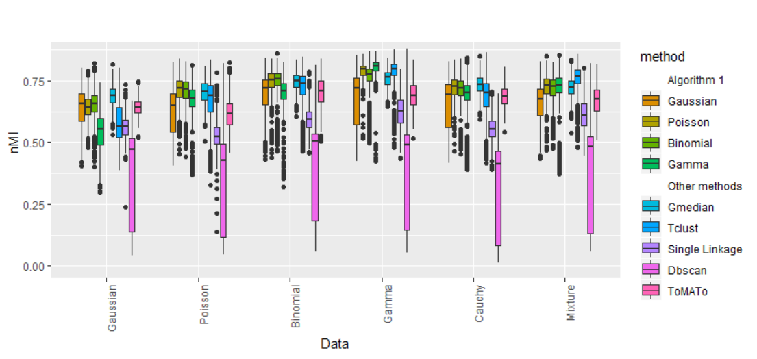
Then we compare the proposed method, in every case, to clustering with other Bregman divergences (including trimmed kk-means [16]), trimmed kk-median [9], tclust [22], and density/distance functions-based clustering schemes such as a robustified version of the classical single linkage procedure, the ToMATo algorithm [14] with the inverse of the distance-to-measure function [12] and dbscan [25]. Details concerning these methods are available in Section 11.1.1. Quality of partitions is assessed via the normalized mutual information (NMI, [36]) with respect to the ground truth clustering, where the “noise" points are assigned to one same cluster.
Refer to caption
Figure 3: Comparison of robust clustering methods, for mixtures of Binomial, Gamma, Gaussian, Poisson, Cauchy, and heterogeneous distributions.

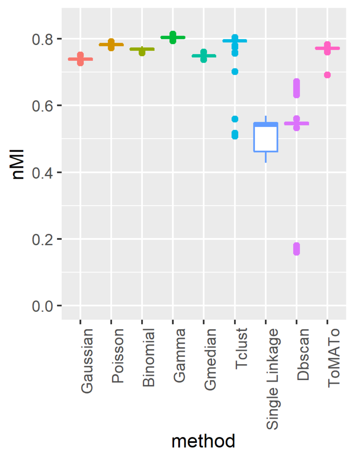
This experiment is repeated 10001000 times, the results in terms of NMI’s are exposed in Figure 9: Algorithm 1 refers to our method with q=110q=110 and k=3k=3. For the Cauchy and heterogeneous distributions, the Gaussian divergence is less efficient, since the 3 clusters have increasing variances. This divergence is well suited for clusters with the same variance, the Gamma and Poisson divergence for data with increasing variance, the Binomial divergence for data with increasing and then decreasing variances, for the proper parameter NN. It is also possible to choose a different Bregman divergence for the different coordinates. Further explanations and numerical illustrations are available in Section 11.2. Choosing between a Gamma or a Poisson divergence depends on the knowledge on the data, as illustrated in the following section with two different real datasets. Note that Algorithm 1 with the proper Bregman divergence (almost) systematically outperforms other clustering schemes. This point is confirmed in Section 11.1.2 for large datasets (n=12000n=12000).

4.5 Daily waterfall data

We consider the daily rainfalls (expressed in mm) for january (241241 data points) and september (8888 data points), from 2007 to 2017, in Cayenne/Rochambeau. Datapoints are defined as the amount of rain within a rainy day. According to [15], the positive daily rainfalls within one month are often modeled as Gamma distribution with parameters depending on the month. We experiment Algorithm 1 with the Gamma and the Gaussian Bregman divergences (the latter is plain trimmed kk-means). The NMI’s between the true labels (i.e. the month from which the datapoint was extracted) and the labels returned by the algorithm for different trimming parameters qq are depicted in the right panel of Figure 4. When qq is small, the Gaussian divergence yields better NMI’s than Gamma. In this case, outliers are considered as a significant cluster in the computation of the NMI. Thus, the “outlier” cluster associated with Gaussian divergence seems closer to a real cluster than the Gamma one. When qq is large enough (small amount of outliers), the clustering associated with Gamma divergence outperforms the Gaussian clustering. The left panel of Figure 4 depicts the associated clustering, for q=300q=300. Of course we cannot expect a perfect clustering since the true clusters are not well-separated. However, it seems that the Gamma divergence clustering allows to consider small precipitations as outliers, contrary to the Gaussian case. This point can be further exploited to choose in practice an appropriate Bregman divergence for to the data to be clustered. For instance, in the case of positive data points, if noise points are expected close to zero, then a Poisson or Gamma divergence might be more suitable than a Gaussian one. Again, the choice of an appropriate Bregman divergence depends on prior knowledge on the structure of data and noise.

Refer to caption
Refer to caption
Refer to caption
Figure 4: From left to right: Clustering with Gaussian divergence and q=300q=300. Clustering with Gamma divergence and q=300q=300. NMI as a function of the trimming parameter qq.

4.6 Authors stylometric clustering

In this Section we perform clustering on texts based on stylometric descriptors exposed in [38, Section 10]. To be more precise, raw data consist in 2626 annotated texts from 44 authors (Mark Twain, Sir Arthur Conan Doyle, Nathaniel Hawthorne and Charles Dickens). These texts are available as supplementary material for [38], and are framed as a sequence of lemmatized string characters (for instance "be" and "is" are instances of the same lemma "be"). Following [38], we base our stylometric comparison on lemmas corresponding to nouns, verbs and adverbs, and split every original text in chunks of size 50005000 of such lemmas that will be considered as data points. Then the 5050 overall most frequent lemmas are chosen, and every chunk is described as the vector of counts of these lemmas within it. Thus, signal points consists of 189189 count vectors with dimension 5050, originating from 44 different authors.

The signal points are corrupted using the same process for the 88 State of the Union Addresses given by Barack Obama (available in obama dataset from package CleanNLP in R), resulting in 55 additional points, and for the King James Version of the Bible (available on Project Gutenberg) that we preliminary lemmatize using the CleanNLP package, resulting in 1515 more additional points. Our final dataset consists of the 189189 signal points and the 2020 outlier points described above. Slightly anticipating, these 2020 outliers might also be thought of as two additional small clusters with size 55 and 1515.

Since every individual lemma count can be modeled as a Poisson random variable in the random character sequence model [20], the appropriate Bregman divergence for this dataset is likely to be the Poisson divergence. In the following, we compare our method with Poisson divergence to trimmed kk-means, trimmed kk-medians, and tt-clust.

Refer to caption
Figure 5: Cost curves for authors clustering with Poisson divergence.

In Figure 5, we draw the cost of our method as a function of qq, for different cluster numbers kk. According to this figure, several choices of kk and qq are possible. For values of qq up to 175175, the significant jumps in the risk function are for k=3k=3 and k=6k=6. For k=3k=3, the slope heuristic yields q=175q=175, whereas for k=6k=6 the slope heuristic suggests that no data points might be considered as outliers. When qq ranges between 175175 and 193193, the significant distortion jumps are for k=4k=4 and k=6k=6, another possible choice is then k=4k=4 and q=188q=188. When qq is larger than 193193, the only significant jump is for k=6k=6. To summarize, the pairs (k=3,q=175)(k=3,q=175), (k=4,q=188)(k=4,q=188), (k=6,q=n=209)(k=6,q=n=209) seem reasonable. These three solutions correspond to the 3 natural trimmed partitions: clustering only 33 authors writings (Twain writings being considered as outliers), clustering the 4 authors writings and removing the outliers from the Bible and B. Obama addresses, and at last clustering the six sources of writings (none of them being considered as noise). The two latter situations are depicted in Figure 6, in the 22-dimensional basis given by a linear discriminant analysis of the proposed clustering.

Refer to caption
Refer to caption
Figure 6: Author stylometric clustering with Poisson divergence.

For k=6k=6 and q=209q=209, our clustering globally retrieves the corresponding author. When k=4,q=188k=4,q=188 is chosen, outliers are correctly identified and only one sample text from C. Dickens is labeled as outlier. The sample points seem on the whole well classified, that is assessed by a NMI of 0.73470.7347. This performance is compared with the other clustering algorithms in Table 2. Note that values of qq have been chosen to minimize the NMI, leading to q=190q=190 for trimmed kk-means, q=202q=202 for trimmed kk-medians, and q=184q=184 for tclust. The NMI curves may be found in Section 11.

Method trimmed 44-means trimmed 44-medians tclust Poisson
NMI 0.53360.5336 0.43340.4334 0.49130.4913 0.73470.7347
Table 2: Comparison of robust clustering methods for Author retrieving.

The associated partitions for kk-median and tclust are depicted in Figure 7, showing that these two methods fail in correctly identifying outliers.

Refer to caption
Refer to caption
Figure 7: Author stylometric clustering with trimmed kk-median and tclust.

5 Proofs for Section 2

5.1 Intermediate results

The proofs of Theorem 8, Theorem 10 and Theorem 11 make extensive use of the following lemmas, whose proofs are deferred to Section 9. The first of them is a global upper bound on the radii rh​(c)r_{h}(c), when cc is in a compact subset of Ω\Omega.

Lemma 20.

Assume that ϕ\phi is 𝒞2\mathcal{C}^{2} and F0=c​o​n​v​(s​u​p​p​(P))¯⊂Ω̊F_{0}=\overline{conv(supp(P))}\subset\mathring{\Omega}. Then, for every h∈(0,1)h\in(0,1) and K>0K>0, there exists r+<∞r^{+}<\infty such that

supc∈F0∩B¯​(0,K),s≤hrs​(c)≤r+.\displaystyle\sup_{c\in F_{0}\cap\bar{B}(0,K),s\leq h}r_{s}(c)\leq r^{+}.

As a consequence, if 𝐜\mathbf{c} is a codebook with a codepoint cj0∈F0c_{j_{0}}\in F_{0} satisfying ‖cj0‖≤K\|c_{j_{0}}\|\leq K and s≤hs\leq h, then rs​(𝐜)≤r+r_{s}(\mathbf{c})\leq r^{+}.

Next, the following lemma makes connections between the difference of Bregman divergences and distance between codebooks.

Lemma 21.

Assume that F0⊂Ω̊F_{0}\subset\mathring{\Omega} and ϕ\phi is 𝒞2\mathcal{C}^{2} on Ω\Omega. Then, for every K>0K>0, there exists CK>0C_{K}>0 such that for every 𝐜\mathbf{c} and 𝐜′\mathbf{c}^{\prime} in B¯​(0,K)∩F0\bar{B}(0,K)\cap F_{0}, and x∈Ωx\in\Omega,

|dϕ​(x,𝐜)−dϕ​(x,𝐜′)|≤CK​D​(𝐜,𝐜′)​(1+‖x‖),\left|d_{\phi}(x,\mathbf{c})-d_{\phi}(x,\mathbf{c}^{\prime})\right|\leq C_{K}D(\mathbf{c},\mathbf{c}^{\prime})\left(1+\|x\|\right),

where D⁡(𝐜,𝐜′)=minσ∈Σk⁡maxj∈[[1,k]]​|cj−cσ⁡(j)′|D(\mathbf{c},\mathbf{c}^{\prime})=\min_{\sigma\in\Sigma_{k}}\max_{j\in[\![1,k]\!]}|c_{j}-c^{\prime}_{\sigma(j)}| (cf. Theorem 10).

We will also need a continuity result on the function (s,𝐜)↦Rs​(𝐜)(s,\mathbf{c})\mapsto R_{s}(\mathbf{c}).

Lemma 22.

Assume that F0⊂Ω̊F_{0}\subset\mathring{\Omega}, P​‖u‖<∞P\|u\|<\infty and ϕ\phi is 𝒞2\mathcal{C}^{2} on Ω\Omega. Then the map (s,𝐜)→Rs​(𝐜)(s,\mathbf{c})\rightarrow R_{s}(\mathbf{c}) is continuous. Moreover, for every h∈(0,1)h\in(0,1), ϵ>0\epsilon>0 and K>0K>0, there is s0<hs_{0}<h such that

∀s0<s<h,sup𝐜∈(F0∩B¯​(0,K))(k)Rh​(𝐜)−Rs​(𝐜)≤ϵ.\forall s_{0}<s<h,\,\sup_{\mathbf{c}\in\left(F_{0}\cap\bar{B}(0,K)\right)^{(k)}}R_{h}(\mathbf{c})-R_{s}(\mathbf{c})\leq\epsilon.

5.2 Proof of Lemma 5

Set 0<h<h′<10<h<h^{\prime}<1, and recall that F𝐜−1​(u)=ru2​(𝐜)F_{\mathbf{c}}^{-1}(u)=r^{2}_{u}(\mathbf{c}) denotes the uu-quantile of the random variable dϕ​(X,𝐜)d_{\phi}(X,\mathbf{c}) for X∼PX\sim P and u∈[0,1]u\in[0,1]. Since F𝐜−1F_{\mathbf{c}}^{-1} is non-decreasing, we may write

Rh​(𝐜)h=∫01F𝐜−1​(h​u)​𝑑u≤∫01F𝐜−1​(h′​u)​𝑑u=Rh′​(𝐜)h′.\displaystyle\frac{R_{h}(\mathbf{c})}{h}=\int_{0}^{1}F_{\mathbf{c}}^{-1}(hu)du\leq\int_{0}^{1}F_{\mathbf{c}}^{-1}(h^{\prime}u)du=\frac{R_{h^{\prime}}(\mathbf{c})}{h^{\prime}}.

Equality holds if and only if F𝐜−1​(h​u)=F𝐜−1​(h′​u)F_{\mathbf{c}}^{-1}(hu)=F_{\mathbf{c}}^{-1}(h^{\prime}u) for almost all u∈[0,1]u\in[0,1]. Since F𝐜−1F_{\mathbf{c}}^{-1} is non-decreasing, L𝐜:=liml′→0F𝐜−1​(l′)L_{\mathbf{c}}:=\lim_{l^{\prime}\rightarrow 0}F_{\mathbf{c}}^{-1}(l^{\prime}) exists. Moreover, for l<h′l<h^{\prime}, F𝐜−1​(h​u)=F𝐜−1​(h′​u)F_{\mathbf{c}}^{-1}(hu)=F_{\mathbf{c}}^{-1}(h^{\prime}u) a.s., and F𝐜−1​(l)=limn→∞F𝐜−1​((h/h′)n​l)=L𝐜F_{\mathbf{c}}^{-1}(l)=\lim_{n\rightarrow\infty}F_{\mathbf{c}}^{-1}\left((h/h^{\prime})^{n}l\right)=L_{\mathbf{c}}, that is, rl2​(𝐜)=liml′→0rl′2​(𝐜)r^{2}_{l}(\mathbf{c})=\lim_{l^{\prime}\rightarrow 0}r^{2}_{l^{\prime}}(\mathbf{c}). From (1), it follows that P⁡(Bϕ​(𝐜,rh′​(𝐜)))=0P(B_{\phi}(\mathbf{c},r_{h^{\prime}}(\mathbf{c})))=0. Conversely, equality holds when P⁡(Bϕ​(𝐜,rh′​(𝐜)))=0P(B_{\phi}(\mathbf{c},r_{h^{\prime}}(\mathbf{c})))=0. ∎

5.3 Proof of Theorem 8

The intuition behind the proof of Theorem 8 is that optimal codebooks satisfy a so-called centroid condition, namely their code points are means of their trimmed Bregman-Voronoi cells. Thus, provided that optimal Bregman-Voronoi cells have enough weight, the assumption P​‖u‖<+∞P\|u\|<+\infty leads to a bound on the norm of these code points. This idea is summarized by the following lemma, that is also a key ingredient in the proofs of the results of Section 3.

Lemma 23.

Assume that the requirements of Theorem 8 are satisfied. For every k≥2k\geq 2, if Rk−1,h∗−Rk,h∗>0R^{*}_{k-1,h}-R^{*}_{k,h}>0, then

α:=minj∈[[2,k]]⁡Rj−1,h∗−Rj,h∗>0.\alpha:=\min_{j\in[\![2,k]\!]}R^{*}_{j-1,h}-R^{*}_{j,h}>0.

Moreover there exist h−,h+∈(0,1)h^{-},h^{+}\in(0,1) with h∈(h−,h+)h\in(h^{-},h^{+}) such that, for every j∈[[2,k]]j\in[\![2,k]\!], Rj−1,h−∗−Rj,h+∗≥α2R^{*}_{j-1,h^{-}}-R^{*}_{j,h^{+}}\geq\frac{\alpha}{2}.

For every b∈(0,h∧(1−h)]b\in(0,h\wedge(1-h)], set hb−=(h−b)/(1−b)h_{b}^{-}=(h-b)/(1-b) and hb+=h/(1−b)h_{b}^{+}=h/(1-b). Let bb be such that minj∈[[2,k]]⁡Rj−1,hb−∗−Rj,hb+∗>0\min_{j\in[\![2,k]\!]}R^{*}_{j-1,h_{b}^{-}}-R^{*}_{j,h_{b}^{+}}>0, and, for κ1\kappa_{1} in (0,1)(0,1), set b1=κ1​bb_{1}=\kappa_{1}b. Then, for every s∈[hb1−,hb1+]s\in[h_{b_{1}}^{-},h_{b_{1}}^{+}] and j∈[[1,k]]j\in[\![1,k]\!], there exists a minimizer 𝐜j,s∗\mathbf{c}^{*}_{j,s} of Rj,sR_{j,s} satisfying

∀p∈[[1,j]],‖cj,s,p∗‖≤P​‖u‖b⁡(1−h)​(1−κ1).\forall p\in[\![1,j]\!],\quad\|c^{*}_{j,s,p}\|\leq\frac{P\|u\|}{b(1-h)(1-\kappa_{1})}.

The proof of Lemma 23 is deferred to Section 9. When Rk−1,h∗−Rk,h∗>0R^{*}_{k-1,h}-R^{*}_{k,h}>0, Theorem 8 follows from Lemma 23. In the case where Rk−1,h∗−Rk,h∗=0R^{*}_{k-1,h}-R^{*}_{k,h}=0, there exists a set AA with P⁡(A)≥hP(A)\geq h such that the restriction of PP to AA is supported by at most k−1k-1 points. These k−1k-1 points provide an optimal kk-points codebook. Hence the result of Theorem 8. ∎

5.4 Proof of Proposition 14

The first part of Proposition 14 follows from Lemma 23. Indeed, if h−h^{-} and h+h^{+} are such that minj∈[[2,k]]⁡Rj−1,h−∗−Rj,h+∗>0\min_{j\in[\![2,k]\!]}R^{*}_{j-1,h^{-}}-R^{*}_{j,h^{+}}>0, then for bb small enough so that h−≤hb−<h<hb+≤h+h^{-}\leq h_{b}^{-}<h<h_{b}^{+}\leq h^{+}, we have minj∈[[2,k]]⁡Rj−1,hb−∗−Rj,hb+∗≥minj∈[[2,k]]⁡Rj−1,h−∗−Rj,h+∗>0\min_{j\in[\![2,k]\!]}R^{*}_{j-1,h_{b}^{-}}-R^{*}_{j,h_{b}^{+}}\geq\min_{j\in[\![2,k]\!]}R^{*}_{j-1,h^{-}}-R^{*}_{j,h^{+}}>0.

We turn to the second part of Proposition 14. Let 𝐜∗,(j)\mathbf{c}^{*,(j)} be a jj-points hh-trimmed optimal codebook, and pj,h=h​minl∈[[1,j]]​P~𝐜∗,(j)​(Wl​(𝐜∗,(j)))p_{j,h}=h\min_{l\in[\![1,j]\!]}\tilde{P}_{\mathbf{c}^{*,(j)}}\left(W_{l}(\mathbf{c}^{*,(j)})\right), where P~𝐜∗,(j)∈𝒫h​(𝐜∗,(j))\tilde{P}_{\mathbf{c}^{*,(j)}}\in\mathcal{P}_{h}(\mathbf{c}^{*,(j)}). Let τj,h\tau_{j,h} denote the [0,1][0,1]-valued function such that h​P~𝐜∗,(j)=P​τj,hh\tilde{P}_{\mathbf{c}^{*,(j)}}=P\tau_{j,h}. Assume that pj,h=P​τj,h​(u)​𝟙W1​(𝐜∗,(j))​(u)p_{j,h}=P\tau_{j,h}(u)\mathbbm{1}_{W_{1}(\mathbf{c}^{*,(j)})}(u), without loss of generality. Then we have

Rj,h∗≥∑l=2kP​dϕ​(u,cl∗,(j))​(u)​τj,h​(u)​𝟙Wl​(𝐜∗,(j))​(u)≥Rj−1,h−pj,h∗.\displaystyle R^{*}_{j,h}\geq\sum_{l=2}^{k}Pd_{\phi}(u,c^{*,(j)}_{l})(u)\tau_{j,h}(u)\mathbbm{1}_{W_{l}(\mathbf{c}^{*,(j)})}(u)\geq R^{*}_{j-1,h-p_{j,h}}.

Thus, (h−Bh)/(1−Bh)≥h−pj,h(h-B_{h})/(1-B_{h})\geq h-p_{j,h}, that entails (1−(h−pj,h))​Bh≤pj,h(1-(h-p_{j,h}))B_{h}\leq p_{j,h}.

6 Proofs for Section 3

6.1 Intermediate results

Theorem 10 and 11 require some additional probabilistic results that are gathered in this subsection. Some of them are applications of standard techniques, their proofs are thus deferred to Section 10, for the sake of completeness. We begin with deviation bounds.

Proposition 24.

With probability larger than 1−e−x1-e^{-x}, we have, for k≥2k\geq 2,

sup𝐜∈(ℝd)(k),r≥0|(P−Pn)​𝟙Bϕ​(𝐜,r)|\displaystyle\sup_{\mathbf{c}\in(\mathbb{R}^{d})^{(k)},r\geq 0}\left|(P-P_{n})\mathbbm{1}_{B_{\phi}(\mathbf{c},r)}\right| ≤C​k⁡(d+1)​log⁡(k)n+2​xn,\displaystyle\leq C\sqrt{\frac{k(d+1)\log(k)}{n}}+\sqrt{\frac{2x}{n}}, (2)
sup𝐜∈(ℝd)(k),r≥0|(P−Pn)​𝟙∂Bϕ​(𝐜,r)|\displaystyle\sup_{\mathbf{c}\in(\mathbb{R}^{d})^{(k)},r\geq 0}\left|(P-P_{n})\mathbbm{1}_{\partial B_{\phi}(\mathbf{c},r)}\right| ≤C​k⁡(d+1)​log⁡(k)n+2​xn,\displaystyle\leq C\sqrt{\frac{k(d+1)\log(k)}{n}}+\sqrt{\frac{2x}{n}},

where ∂Bϕ​(𝐜,r)\partial B_{\phi}(\mathbf{c},r) denotes {x∣dϕ​(x,𝐜)=r2}\left\{x\mid d_{\phi}(x,\mathbf{c})=r^{2}\right\} and CC denotes a universal constant. Moreover, if r+r^{+} and KK are fixed, and P​‖u‖2≤M22<∞P\|u\|^{2}\leq M_{2}^{2}<\infty, we have, with probability larger than 1−e−x1-e^{-x},

sup𝐜∈(B¯​(0,K)∩F0)(k),r≤r+|(P−Pn)dϕ(.,𝐜)𝟙Bϕ​(𝐜,r)|\displaystyle\sup_{\mathbf{c}\in\left(\bar{B}(0,K)\cap F_{0}\right)^{(k)},r\leq r^{+}}\left|(P-P_{n})d_{\phi}(.,\mathbf{c})\mathbbm{1}_{B_{\phi}(\mathbf{c},r)}\right| ≤(r+)2​[CK,r+,M2​k​d​log⁡(k)n+2​xn],\displaystyle\leq(r^{+})^{2}\left[C_{K,r^{+},M_{2}}\frac{\sqrt{kd\log(k)}}{\sqrt{n}}+\sqrt{\frac{2x}{n}}\right], (3)
sup𝐜∈(B¯​(0,K)∩F0)(k),r≤r+|(P−Pn)dϕ(.,𝐜)𝟙∂Bϕ​(𝐜,r)|\displaystyle\sup_{\mathbf{c}\in\left(\bar{B}(0,K)\cap F_{0}\right)^{(k)},r\leq r^{+}}\left|(P-P_{n})d_{\phi}(.,\mathbf{c})\mathbbm{1}_{\partial B_{\phi}(\mathbf{c},r)}\right| ≤(r+)2​[CK,r+,M2​k​d​log⁡(k)n+2​xn],\displaystyle\leq(r^{+})^{2}\left[C_{K,r^{+},M_{2}}\frac{\sqrt{kd\log(k)}}{\sqrt{n}}+\sqrt{\frac{2x}{n}}\right],

where we recall that c​o​n​v​(s​u​p​p​(P))¯=F0⊂Ω̊\overline{conv(supp(P))}=F_{0}\subset\mathring{\Omega}.

A key intermediate result shows that, on the probability events defined above, empirical risk minimizers must have bounded codepoints.

Proposition 25.

Assume that P​‖u‖p<+∞P\|u\|^{p}<+\infty for some p≥2p\geq 2, and let b>0b>0 be such that minj∈[[2,k]]⁡Rj−1,hb−∗−Rj,hb+∗>0\min_{j\in[\![2,k]\!]}R^{*}_{j-1,h_{b}^{-}}-R^{*}_{j,h_{b}^{+}}>0, where hb−=(h−b)/(1−b)h_{b}^{-}=(h-b)/(1-b), hb+=h/(1−b)h^{+}_{b}=h/(1-b), as in Lemma 23. Let κ2<1\kappa_{2}<1, and denote by b2=κ2​bb_{2}=\kappa_{2}b. Then there exists CP,h,k,κ2,bC_{P,h,k,\kappa_{2},b} such that, for nn large enough, with probability larger than 1−n−p21-n^{-\frac{p}{2}}, we have, for all j∈[[2,k]]j\in[\![2,k]\!], and i∈[[1,j]]i\in[\![1,j]\!],

suphb2−≤s≤h‖c^j,s,i‖≤CP,h,k,κ2,b,\displaystyle\sup_{h_{b_{2}^{-}}\leq s\leq h}\|\hat{c}_{j,s,i}\|\leq C_{P,h,k,\kappa_{2},b},

where 𝐜^j,s\hat{\mathbf{c}}_{j,s} denotes a jj-points empirical risk minimizer with trimming level ss.

To prove Theorem 10, a more involved version of Markov’s inequality is needed, stated below.

Lemma 26.

If P​‖u‖p<∞P\|u\|^{p}<\infty for some p≥2p\geq 2, then there exists some positive constant CC such that with probability larger than 1−n−p21-n^{-\frac{p}{2}}, Pn​‖u‖≤CP_{n}\|u\|\leq C.

At last, a technical lemma on empirical quantiles of Bregman divergences will be needed.

Lemma 27.

Let (Pn)n∈ℕ(P_{n})_{n\in\mathbb{N}} be a sequence of probabilities that converges weakly to a distribution PP. Assume that s​u​p​p​(Pn)⊂s​u​p​p​(P)⊂ℝdsupp(P_{n})\subset supp(P)\subset\mathbb{R}^{d}, F0=c​o​n​v​(s​u​p​p​(P))¯⊂Ω̊F_{0}=\overline{conv(supp(P))}\subset\mathring{\Omega} and ϕ\phi is 𝒞2\mathcal{C}_{2} on Ω\Omega. Then, for every h∈(0,1)h\in(0,1) and K>0K>0, there exists K+>0K_{+}>0 such that for every 𝐜∈Ω(k)\mathbf{c}\in\Omega^{(k)} satisfying |ci|≤K|c_{i}|\leq K for some i∈[[1,k]]i\in[\![1,k]\!] and every n∈ℕn\in\mathbb{N},

rn,h​(𝐜)≤r+=4​(2​K+K+)​supc∈F0∩B¯​(0,2​K+K+)‖∇cϕ‖.r_{n,h}(\mathbf{c})\leq r_{+}=\sqrt{4(2K+K_{+})\sup_{c\in F_{0}\cap\bar{B}(0,2K+K_{+})}\|\nabla_{c}\phi\|}.

6.2 Proof of Theorem 10

The proof of Theorem 10 is an adaptation of the proof of [16, Theorem 3.4]. First note that since ϕ\phi is strictly convex and continuous, ψ:x↦ϕ⁡(x)−⟨x,a⟩+b\psi:x\mapsto\phi(x)-\langle x,a\rangle+b is also strictly convex and continuous, for every aa, bb. Thus ψ−1​({0})\psi^{-1}(\{0\}) is a closed set. Moreover, since ψ\psi is strictly convex, any line that contains 00 contains at most two points of ψ−1​({0})\psi^{-1}(\{0\}). Thus, the Lebesgue measure of ψ−1​({0})\psi^{-1}(\{0\}) is 00. Since PP is absolutely continuous, it follows that boundaries of Bregman balls have PP-mass equal to 00.

According to Proposition 25, provided that P​‖u‖p<+∞P\|u\|^{p}<+\infty, for some p>2p>2, there exists CP>0C_{P}>0 such that for some N∈ℕN\in\mathbb{N}, ∑n≥NP⁡(maxi∈[[1,k]]⁡‖c^n,h,i‖>CP)<∞\sum_{n\geq N}P(\max_{i\in[\![1,k]\!]}\left\|\hat{c}_{n,h,i}\right\|>C_{P})<\infty. Thus, the Borel-Cantelli Lemma ensures that, a.s. for nn large enough, for every i∈[[1,k]]i\in[\![1,k]\!], ‖c^n,h,i‖≤CP\left\|\hat{c}_{n,h,i}\right\|\leq C_{P}. According to the Skorokhod’s representation theorem in the Polish space ℝd\mathbb{R}^{d}, there exists a measured space (Ω~,ℱ~,P~)(\tilde{\Omega},\tilde{\mathcal{F}},\tilde{P}) and a sequence of random variables (Xn)n∈ℕ(X_{n})_{n\in\mathbb{N}} along with a random variable XX on (Ω~,ℱ~,P~)(\tilde{\Omega},\tilde{\mathcal{F}},\tilde{P}) such that Xn∼PnX_{n}\sim P_{n}, X∼PX\sim P and XnX_{n} converges to XX P~\tilde{P}-a.s.

Denote by 𝐜∗\mathbf{c}^{*} a minimizer of 𝐜↦Vϕ,hP​(𝐜)\mathbf{c}\mapsto\rm V\it^{P}_{\phi,h}(\mathbf{c}), rn′=rn,h​(𝐜∗)r^{\prime}_{n}=r_{n,h}(\mathbf{c}^{*}) and τn′\tau^{\prime}_{n} a [0,1][0,1]-valued measurable function such that h​Pn,𝐜∗,h=Pn​τn′hP_{n,\mathbf{c}^{*},h}=P_{n}\tau^{\prime}_{n}, that is, such that Pn​τn′​(u)=hP_{n}\tau^{\prime}_{n}(u)=h and

𝟙Bϕ​(𝐜∗,rn′)≤τn′≤𝟙B¯ϕ​(𝐜∗,rn′).\mathbbm{1}_{B_{\phi}(\mathbf{c}^{*},r^{\prime}_{n})}\leq\tau^{\prime}_{n}\leq\mathbbm{1}_{\bar{B}_{\phi}(\mathbf{c}^{*},r^{\prime}_{n})}.

According to Lemma 27, with K=‖c1∗‖K=\|c^{*}_{1}\| for instance, it comes rn′≤r+r^{\prime}_{n}\leq r^{+}, for some finite r+r^{+}. Thus, up to extracting a subsequence, we may assume that rn′→r0′r^{\prime}_{n}\rightarrow r^{\prime}_{0} for some r0′≤r+r^{\prime}_{0}\leq r_{+}. Moreover, it holds

|dϕ​(Xn,𝐜∗)−dϕ​(X,𝐜∗)|≤|ϕ⁡(Xn)−ϕ⁡(X)|+maxj∈[[1,k]]⁡‖∇cj∗ϕ‖​|Xn−X|.\left|d_{\phi}(X_{n},\mathbf{c}^{*})-d_{\phi}(X,\mathbf{c}^{*})\right|\leq|\phi(X_{n})-\phi(X)|+\max_{j\in[\![1,k]\!]}\|\nabla_{c^{*}_{j}}\phi\||X_{n}-X|. (4)

Thus, dϕ​(Xn,𝐜∗)→dϕ​(X,𝐜∗)d_{\phi}(X_{n},\mathbf{c}^{*})\rightarrow d_{\phi}(X,\mathbf{c}^{*}) a.e. when n→∞n\rightarrow\infty. As a consequence, τn′​(Xn)→𝟙Bϕ​(𝐜∗,r0′)​(X)\tau^{\prime}_{n}(X_{n})\rightarrow\mathbbm{1}_{B_{\phi}(\mathbf{c}^{*},r^{\prime}_{0})}(X) P~\tilde{P}-a.e. The dominated convergence theorem yields h=Pn​τn′​(u)→P⁡(Bϕ​(𝐜∗,r0′))h=P_{n}\tau^{\prime}_{n}(u)\rightarrow P(B_{\phi}(\mathbf{c}^{*},r^{\prime}_{0})). Thus, 𝟙Bϕ​(𝐜∗,r0′)=τ0\mathbbm{1}_{B_{\phi}(\mathbf{c}^{*},r^{\prime}_{0})}=\tau_{0} PP-a.e where τ0\tau_{0} denotes the trimming set associated with 𝐜∗\mathbf{c}^{*} and PP. Moreover, since τn′​(Xn)​dϕ​(Xn,𝐜∗)\tau^{\prime}_{n}(X_{n})d_{\phi}(X_{n},\mathbf{c}^{*}) is bounded by r+r_{+} and converges to τ0​(X)​dϕ​(X,𝐜∗)\tau_{0}(X)d_{\phi}(X,\mathbf{c}^{*}) a.e., the dominated convergence theorem entails

Rn,h​(𝐜^n)≤Rn,h​(𝐜∗)≤𝔼⁡[τn′​(Xn)​dϕ​(Xn,𝐜∗)]→𝔼⁡[τ0​(X)​dϕ​(X,𝐜∗)].R_{n,h}(\hat{\mathbf{c}}_{n})\leq R_{n,h}(\mathbf{c}^{*})\leq\mathbb{E}\left[\tau^{\prime}_{n}(X_{n})d_{\phi}(X_{n},\mathbf{c}^{*})\right]\rightarrow\mathbb{E}\left[\tau_{0}(X)d_{\phi}(X,\mathbf{c}^{*})\right].

Thus, lim supn→∞Rn,h​(𝐜^n)≤Rk,h∗\limsup_{n\rightarrow\infty}R_{n,h}(\hat{\mathbf{c}}_{n})\leq R_{k,h}^{*}.

Since, for n≥Nn\geq N and every i∈[[1,k]]i\in[\![1,k]\!], ‖c^n,i‖≤CP\|\hat{c}_{n,i}\|\leq C_{P}, we have c^u⁡(n),i→ci\hat{c}_{u(n),i}\rightarrow c_{i} for some ci∈F0∩B¯​(0,CP)c_{i}\in F_{0}\cap\bar{B}(0,C_{P}), where 𝐜^u⁡(n)\hat{\mathbf{c}}_{u(n)} is a subsequence. Set 𝐜=(c1,c2,…,ck)\mathbf{c}=(c_{1},c_{2},\dots,c_{k}). Again, according to Lemma 27 with K=CPK=C_{P}, it comes that ru⁡(n),h​(𝐜^u⁡(n))→rr_{u(n),h}(\hat{\mathbf{c}}_{u(n)})\rightarrow r for some r≥0r\geq 0. Therefore, from (4), Lemma 21 and the continuity of PP,

limn→∞τu⁡(n)​(Xu⁡(n))=𝟙Bϕ​(𝐜,r)​(X)a.e.,\lim_{n\rightarrow\infty}\tau_{u(n)}(X_{u(n)})=\mathbbm{1}_{B_{\phi}(\mathbf{c},r)}(X)\quad a.e.,

where τu⁡(n)=𝟙Bϕ​(𝐜^u⁡(n),ru⁡(n),h​(𝐜^u⁡(n)))\tau_{u(n)}=\mathbbm{1}_{B_{\phi}(\hat{\mathbf{c}}_{u(n)},r_{u(n),h}(\hat{\mathbf{c}}_{u(n)}))}. According to the dominated convergence theorem, we have h=P⁡(Bϕ​(𝐜,r))=Pu⁡(n)​(τu⁡(n)​(u))h=P(B_{\phi}(\mathbf{c},r))=P_{u(n)}(\tau_{u(n)}(u)). Again, the dominated convergence theorem implies that

liminfn→∞Ru⁡(n),h​(𝐜^u⁡(n))≥P​𝟙Bϕ​(𝐜,r)​(u)​dϕ​(u,𝐜)=Rh​(𝐜)≥Rk,h∗.\lim\inf_{n\rightarrow\infty}R_{u(n),h}(\hat{\mathbf{c}}_{u(n)})\geq P\mathbbm{1}_{B_{\phi}(\mathbf{c},r)}(u)d_{\phi}(u,\mathbf{c})=R_{h}(\mathbf{c})\geq R^{*}_{k,h}.

As a consequence, limn→∞Ru⁡(n),h​(𝐜^u⁡(n))=Rh​(𝐜)=Rk,h∗\lim_{n\rightarrow\infty}R_{u(n),h}(\hat{\mathbf{c}}_{u(n)})=R_{h}(\mathbf{c})=R_{k,h}^{*} and 𝐜\mathbf{c} is an optimal trimmed codebook. Since, given a subsequence of (𝐜^n)n∈ℕ(\hat{\mathbf{c}}_{n})_{n\in\mathbb{N}}, we may find a subsequence of indices u⁡(n)u(n) such that limn→∞Ru⁡(n),h​(𝐜^u⁡(n))=Rk,h∗\lim_{n\rightarrow\infty}R_{u(n),h}(\hat{\mathbf{c}}_{u(n)})=R_{k,h}^{*}, we deduce that limn→+∞Rn,h​(𝐜^n)=Rk,h∗\lim_{n\rightarrow+\infty}R_{n,h}(\hat{\mathbf{c}}_{n})=R^{*}_{k,h}.

Now assume that 𝐜h∗\mathbf{c}^{*}_{h} is unique. Then, for every subsequence of (𝐜^n)n∈ℕ(\hat{\mathbf{c}}_{n})_{n\in\mathbb{N}}, there exists u⁡(n)u(n) such that 𝐜^u⁡(n)→𝐜=𝐜h∗\hat{\mathbf{c}}_{u(n)}\rightarrow\mathbf{c}=\mathbf{c}^{*}_{h}. Thus, a.e., 𝐜^n→𝐜h∗\hat{\mathbf{c}}_{n}\rightarrow\mathbf{c}^{*}_{h}. ∎

6.3 Proof of Theorem 11

For h>0h>0 and a codebook 𝐜\mathbf{c}, we denote by τh​(𝐜)\tau_{h}(\mathbf{c}) the trimming function 𝟙Bϕ​(𝐜,rh​(𝐜))+δh​(𝐜)​𝟙∂Bϕ​(𝐜,rh​(𝐜))\mathbbm{1}_{B_{\phi}(\mathbf{c},r_{h}(\mathbf{c}))}+\delta_{h}(\mathbf{c})\mathbbm{1}_{\partial B_{\phi}(\mathbf{c},r_{h}(\mathbf{c}))}, so that P​τh​(𝐜)/h∈𝒫h​(𝐜)P\tau_{h}(\mathbf{c})/h\in\mathcal{P}_{h}(\mathbf{c}). We also denote by τ^h​(𝐜)\hat{\tau}_{h}(\mathbf{c}) its empirical counterpart. Note that δh​(𝐜)\delta_{h}(\mathbf{c}) and δ^h​(𝐜)\hat{\delta}_{h}(\mathbf{c}) are smaller than 11. It follows that

|P​τh​(𝐜)−P​τ^h​(𝐜)|\displaystyle|P\tau_{h}(\mathbf{c})-P\hat{\tau}_{h}(\mathbf{c})| =|(P−Pn)​τ^h​(𝐜)|\displaystyle=|(P-P_{n})\hat{\tau}_{h}(\mathbf{c})|
≤|(P−Pn)​Bϕ​(𝐜,rn,h​(𝐜))|+δ^​(𝐜)​|(P−Pn)​∂Bϕ​(𝐜,rn,h​(𝐜))|\displaystyle\leq|(P-P_{n})B_{\phi}(\mathbf{c},r_{n,h}(\mathbf{c}))|+\hat{\delta}(\mathbf{c})|(P-P_{n})\partial B_{\phi}(\mathbf{c},r_{n,h}(\mathbf{c}))|
≤|(P−Pn)​Bϕ​(𝐜,rn,h​(𝐜))|+|(P−Pn)​∂Bϕ​(𝐜,rn,h​(𝐜))|.\displaystyle\leq|(P-P_{n})B_{\phi}(\mathbf{c},r_{n,h}(\mathbf{c}))|+|(P-P_{n})\partial B_{\phi}(\mathbf{c},r_{n,h}(\mathbf{c}))|.

As well, we bound |Pn​τh​(𝐜)−Pn​τ^h​(𝐜)||P_{n}\tau_{h}(\mathbf{c})-P_{n}\hat{\tau}_{h}(\mathbf{c})| the same way. Combining Lemma 23 and Proposition 25, we consider a probability event onto which, for all jj, ‖𝐜^n,j‖≤CP\|\hat{\mathbf{c}}_{n,j}\|\leq C_{P} and sup𝐜∈(F0∩B¯​(0,CP))(k)rn,h​(𝐜)∨rh​(𝐜)≤r+\sup_{\mathbf{c}\in(F_{0}\cap\bar{B}(0,C_{P}))^{(k)}}r_{n,h}(\mathbf{c})\vee r_{h}(\mathbf{c})\leq r^{+}. This occurs with probability at least 1−n−p/21-n^{-p/2} for CPC_{P} and r+r^{+} large enough (more details are given in Section 10.2). We also assume that the deviation bounds of Proposition 24 hold, with parameter CPC_{P} and r+r_{+}, to define a global probability event with mass larger than 1−n−p/2−2e−x1-n^{-p/2}-2e^{-x}. On this event, we have

Rh​(𝐜^n)−Rk,h∗\displaystyle R_{h}(\hat{\mathbf{c}}_{n})-R^{*}_{k,h} =P​dϕ​(u,𝐜^n)​τ^h​(𝐜^n)−P​dϕ​(u,𝐜∗)​τ^h​(𝐜∗)+P​dϕ​(u,𝐜^n)​(τh​(𝐜^n)−τ^h​(𝐜^n)−(P​dϕ​(u,𝐜∗)​(τh​(𝐜∗)−τ^h​(𝐜∗))CLOSECLOSE\displaystyle=\begin{multlined}Pd_{\phi}(u,\hat{\mathbf{c}}_{n})\hat{\tau}_{h}(\hat{\mathbf{c}}_{n})-Pd_{\phi}(u,\mathbf{c}^{*})\hat{\tau}_{h}(\mathbf{c}^{*})\\ +Pd_{\phi}(u,\hat{\mathbf{c}}_{n})(\tau_{h}(\hat{\mathbf{c}}_{n})-\hat{\tau}_{h}(\hat{\mathbf{c}}_{n})-(Pd_{\phi}(u,\mathbf{c}^{*})(\tau_{h}(\mathbf{c}^{*})-\hat{\tau}_{h}(\mathbf{c}^{*}))\end{multlined}
≤2​sup𝐜∈(F0∩B¯​(0,CP))(k),r≤r+|(P−Pn)​dϕ​(u,𝐜)​𝟙Bϕ​(𝐜,r)​(u)|\displaystyle\leq 2\sup_{\mathbf{c}\in(F_{0}\cap\bar{B}(0,C_{P}))^{(k)},r\leq r^{+}}|(P-P_{n})d_{\phi}(u,\mathbf{c})\mathbbm{1}_{B_{\phi}(\mathbf{c},r)}(u)|
+2(r+)2sup𝐜∈Ω(k),r≥0|(P−Pn)Bϕ(𝐜,r)|\displaystyle\quad+2(r^{+})^{2}\sup_{\mathbf{c}\in\Omega^{(k)},r\geq 0}|(P-P_{n})B_{\phi}(\mathbf{c},r)|
+2sup𝐜∈(F0∩B¯​(0,CP))(k),r≤r+|(P−Pn)dϕ(u,𝐜)𝟙∂Bϕ​(𝐜,r)(u)|\displaystyle\quad+2\sup_{\mathbf{c}\in(F_{0}\cap\bar{B}(0,C_{P}))^{(k)},r\leq r^{+}}|(P-P_{n})d_{\phi}(u,\mathbf{c})\mathbbm{1}_{\partial B_{\phi}(\mathbf{c},r)}(u)|
+2(r+)2sup𝐜∈Ω(k),r≥0|(P−Pn)∂Bϕ(𝐜,r)|.\displaystyle\quad+2(r^{+})^{2}\sup_{\mathbf{c}\in\Omega^{(k)},r\geq 0}|(P-P_{n})\partial B_{\phi}(\mathbf{c},r)|.

Therefore, Rh​(𝐜^n)−Rk,h∗≤CP​(1+x)/nR_{h}(\hat{\mathbf{c}}_{n})-R^{*}_{k,h}\leq{C_{P}(1+\sqrt{x})}/{\sqrt{n}}, for some constant CPC_{P}. ∎

6.4 Proof of Corollary 12

Denote by AA the intersection of the probability events described in Proposition 25, that has probability larger than 1−n−p21-n^{-\frac{p}{2}}. Decomposing the excess risk as in the proof of Theorem 11 yields

Rh​(𝐜^n)−Rk,h∗\displaystyle R_{h}(\hat{\mathbf{c}}_{n})-R^{*}_{k,h} =(Rh​(𝐜^n)−Rk,h∗)​𝟙A+(Rh​(𝐜^n)−Rk,h∗)​𝟙Ac.\displaystyle=(R_{h}(\hat{\mathbf{c}}_{n})-R^{*}_{k,h})\mathbbm{1}_{A}+(R_{h}(\hat{\mathbf{c}}_{n})-R^{*}_{k,h})\mathbbm{1}_{A^{c}}.

According to Proposition 24, we have 𝔼⁡((Rh​(𝐜^n)−Rk,h∗)​𝟙A)≤CP/n\mathbb{E}((R_{h}(\hat{\mathbf{c}}_{n})-R^{*}_{k,h})\mathbbm{1}_{A})\leq C_{P}/\sqrt{n}. It only remains to bound the expectation of the second term. This is the aim of the following Lemma, whose proof is deferred to Section 10.5.

Lemma 28.

Assume that P​‖u‖q​ψq​(k​‖u‖/h)<∞P\|u\|^{q}\psi^{q}(k\|u\|/h)<\infty. Then there exists a constant CqC_{q} such that 𝔼​Rhq​(𝐜^n)≤CPq\mathbb{E}R_{h}^{q}(\hat{\mathbf{c}}_{n})\leq C_{P}^{q}.

Equipped with Lemma 28, we may bound 𝔼⁡(Rh​(𝐜^n)​𝟙Ac)\mathbb{E}(R_{h}(\hat{\mathbf{c}}_{n})\mathbbm{1}_{A^{c}}) as follows, using Hölder’s inequality,

𝔼⁡(Rh​(𝐜^n)​𝟙Ac)\displaystyle\mathbb{E}(R_{h}(\hat{\mathbf{c}}_{n})\mathbbm{1}_{A^{c}}) ≤(ℙ⁡(Ac))1p​(𝔼​Rhq​(𝐜^n))1q≤CP/n.\displaystyle\leq\left(\mathbb{P}(A^{c})\right)^{\frac{1}{p}}\left(\mathbb{E}R_{h}^{q}(\hat{\mathbf{c}}_{n})\right)^{\frac{1}{q}}\leq C_{P}/{\sqrt{n}}.

6.5 Proof of Theorem 15

A key ingredient of the proof of Theorem 15 is the following lemma, ensuring that every cell of a trimmed and corrupted empirical distortion minimizer contains a minimal portion of signal points. In what follows, the τ^\hat{\tau}’s are the trimming function with respect to PnP_{n} (uncorrupted sample), as defined in Section 6.3.

Lemma 29.

Assume that Bh>0B_{h}>0 (see Definition 13), let b<Bhb<B_{h} and b<b1<Bhb<b_{1}<B_{h} such that b=κ1​b1b=\kappa_{1}b_{1}, with κ1<1\kappa_{1}<1. Denote by β1=(1−κ1)​b1​[h∧(1−h)]/2\beta_{1}=(1-\kappa_{1})b_{1}\left[h\wedge(1-h)\right]/2. Assume that s/(n+s)≤bs/(n+s)\leq b. Then, for nn large enough, with probability larger than 1−n−p21-n^{-\frac{p}{2}}, we have, for all j∈[[1,k]]j\in[\![1,k]\!],

Pn​(τ^hb−​(𝐜^n+s,h)​𝟙Wj​(𝐜^n+s,h))≥β1.P_{n}\left(\hat{\tau}_{h_{b}^{-}}(\hat{\mathbf{c}}_{n+s,h})\mathbbm{1}_{W_{j}(\hat{\mathbf{c}}_{n+s,h})}\right)\geq\beta_{1}.

The proof of Lemma 29 is postponed to Section 10.6. We are now in a position to prove Theorem 15.

Proof of Theorem 15.

We adopt the same notation and assumptions as in the proof of Lemma 29. We may write

(n+s)​R^n+s,h​(𝐜^n+s,h)\displaystyle(n+s)\hat{R}_{n+s,h}(\hat{\mathbf{c}}_{n+s,h}) ≤n⁡(Rhb++βn∗+αn).\displaystyle\leq n\left(R^{*}_{h_{b}^{+}+\beta_{n}}+\alpha_{n}\right).

On the other hand, recall that for all j∈[[1,k]]j\in[\![1,k]\!], Pn​(τ^hb−​(𝐜^n+s,h)​𝟙Wj​(𝐜^n+s,h))≥β1P_{n}\left(\hat{\tau}_{h_{b}^{-}}(\hat{\mathbf{c}}_{n+s,h})\mathbbm{1}_{W_{j}(\hat{\mathbf{c}}_{n+s,h})}\right)\geq\beta_{1}, and denote by 𝐦=(m1,…,mk)\mathbf{m}=(m_{1},\ldots,m_{k}) the codebook such that

mj=[Pn​(u​τ^hb−​(𝐜^n+s,h)​𝟙Wj​(𝐜^n+s,h))]/[Pn​(τ^hb−​(𝐜^n+s,h)​𝟙Wj​(𝐜^n+s,h))].m_{j}=\left[{P_{n}(u\hat{\tau}_{h_{b}^{-}}(\hat{\mathbf{c}}_{n+s,h})\mathbbm{1}_{W_{j}(\hat{\mathbf{c}}_{n+s,h})})}\right]/\left[{P_{n}\left(\hat{\tau}_{h_{b}^{-}}(\hat{\mathbf{c}}_{n+s,h})\mathbbm{1}_{W_{j}(\hat{\mathbf{c}}_{n+s,h})}\right)}\right].

Then, for all jj, ‖mj‖≤Pn​‖u‖/β1≤CP\|m_{j}\|\leq{P_{n}\|u\|}/{\beta_{1}}\leq C_{P}. Using Proposition 2, we may write

R^n+s,h​(𝐜^n+s,h)\displaystyle\hat{R}_{n+s,h}(\hat{\mathbf{c}}_{n+s,h}) ≥n​R^n,hb−​(𝐜^n+s,h)/(n+s)\displaystyle\geq n\hat{R}_{n,h_{b}^{-}}(\hat{\mathbf{c}}_{n+s,h})/(n+s)
≥nn+s[∑j=1kPn(τ^hb−(𝐜^n+s,h)𝟙Wj​(𝐜^n+s,h))dϕ(mj,c^n+s,h,j)+R^n,hb−(𝐦)].\displaystyle\geq\begin{multlined}\frac{n}{n+s}\left[\sum_{j=1}^{k}P_{n}\left(\hat{\tau}_{h_{b}^{-}}(\hat{\mathbf{c}}_{n+s,h})\mathbbm{1}_{W_{j}(\hat{\mathbf{c}}_{n+s,h})}\right)d_{\phi}(m_{j},\hat{c}_{n+s,h,j})\right.\\ +\left.\vphantom{\sum_{j=1}^{k}}\hat{R}_{n,h^{-}_{b}}(\mathbf{m})\right].\end{multlined}

The last term satisfies

R^n,hb−​(𝐦)\displaystyle\hat{R}_{n,h^{-}_{b}}(\mathbf{m}) ≥Pn​dϕ​(u,𝐦)​τ^hb−​(𝐦)≥Pn​dϕ​(u,𝐦)​τhb−−βn​(𝐦)\displaystyle\geq P_{n}d_{\phi}(u,\mathbf{m})\hat{\tau}_{h_{b}^{-}}(\mathbf{m})\geq P_{n}d_{\phi}(u,\mathbf{m})\tau_{h_{b}^{-}-\beta_{n}}(\mathbf{m})
≥P​dϕ​(u,𝐦)​τhb−−βn​(𝐦)−αn≥Rhb−−βn∗−αn.\displaystyle\quad\geq Pd_{\phi}(u,\mathbf{m})\tau_{h_{b}^{-}-\beta_{n}}(\mathbf{m})-\alpha_{n}\geq R^{*}_{h_{b}^{-}-\beta_{n}}-\alpha_{n}.

Thus, for all j∈[[1,k]]j\in[\![1,k]\!],

β1​dϕ​(mj,c^n+s,h,j)\displaystyle\beta_{1}d_{\phi}(m_{j},\hat{c}_{n+s,h,j}) ≤[2​αn+Rhb++βn∗−Rhb−−βn∗].\displaystyle\leq\left[2\alpha_{n}+R^{*}_{h_{b}^{+}+\beta_{n}}-R^{*}_{h_{b}^{-}-\beta_{n}}\right]. (5)

∎

6.6 Proof of Corollary 16

With the same setting as Theorem 15, according to (5), we have, almost surely, for nn large enough dϕ(K,𝐜^n+s,j)≤2[2αn+Rhb++βn∗−Rhb−−βn∗]/[b(1−κ1)(h∧(1−h)]d_{\phi}(K,\hat{\mathbf{c}}_{n+s,j})\leq 2[2\alpha_{n}+R^{*}_{h_{b}^{+}+\beta_{n}}-R^{*}_{h_{b}^{-}-\beta_{n}}]/[b(1-\kappa_{1})(h\wedge(1-h)], whenever s/(n+s)≤bs/(n+s)\leq b and Bh​κ1>bB_{h}\kappa_{1}>b. Now let cc be defined as

c=sup{r>0∣{x∣dϕ​(K,x)≤r}⊂B⁡(K,1)}.c=\sup\{r>0\mid\{x\mid d_{\phi}(K,x)\leq r\}\subset B(K,1)\}.

If c>0c>0, then requiring bb small enough and s/(n+s)≤bs/(n+s)\leq b ensures that dϕ​(K,𝐜^n+s,j)≤c/2d_{\phi}(K,\hat{\mathbf{c}}_{n+s,j})\leq c/2, almost surely, for nn large enough, hence the result.

Thus, it remains to prove that c>0c>0. Assume that for every r>0r>0, {x∣dϕ​(K,x)≤r}⊈B⁡(K,1)\{x\mid d_{\phi}(K,x)\leq r\}\nsubseteq B(K,1). Then there exists x0∈Kx_{0}\in K and a sequence vnv_{n} satisfying dϕ​(x0,vn)→0d_{\phi}(x_{0},v_{n})\rightarrow 0, along with ‖x0−vn‖>1\|x_{0}-v_{n}\|>1. Noting that, for t≥0t\geq 0, dϕ​(x0,vn+t⁡(vn−x0))≥dϕ​(x0,vn)d_{\phi}(x_{0},v_{n}+t(v_{n}-x_{0}))\geq d_{\phi}(x_{0},v_{n}) yields dϕ​(x0,vn)≥dϕ​(x0,vn′)d_{\phi}(x_{0},v_{n})\geq d_{\phi}(x_{0},v^{\prime}_{n}), where vn′=x0+(vn−x0)/‖vn−x0‖v^{\prime}_{n}=x_{0}+(v_{n}-x_{0})/\|v_{n}-x_{0}\|. Therefore, dϕ​(vn,x0)≥inf‖u−x0‖=1dϕ​(x0,u)>0d_{\phi}(v_{n},x_{0})\geq\inf_{\|u-x_{0}\|=1}d_{\phi}(x_{0},u)>0, hence the contradiction.

At last, if c↦dϕ​(x,c)c\mapsto d_{\phi}(x,c) is a proper map, then dϕ(K,𝐜^n+s,j)≤2[2αn+Rhb++βn∗−Rhb−−βn∗]/[b(1−κ1)(h∧(1−h)]d_{\phi}(K,\hat{\mathbf{c}}_{n+s,j})\leq 2[2\alpha_{n}+R^{*}_{h_{b}^{+}+\beta_{n}}-R^{*}_{h_{b}^{-}-\beta_{n}}]/[b(1-\kappa_{1})(h\wedge(1-h)], whenever s/(n+s)≤bs/(n+s)\leq b and Bh​κ1>bB_{h}\kappa_{1}>b entails that, almost surely, for nn large enough, ‖𝐜^n+s‖2<+∞\|\hat{\mathbf{c}}_{n+s}\|_{2}<+\infty, thus B​P^n,h>b\widehat{BP}_{n,h}>b. Hence B​P^n,h≥Bh\widehat{BP}_{n,h}\geq B_{h}, almost surely for nn large enough. ∎

References

  • [1] David Arthur and Sergei Vassilvitskii “k-means++: the advantages of careful seeding” In Proceedings of the Eighteenth Annual ACM-SIAM Symposium on Discrete Algorithms ACM, New York, 2007, pp. 1027–1035
  • [2] A. Banerjee, X. Guo and H. Wang “On the optimality of conditional expectation as a Bregman predictor” In IEEE Transactions on Information Theory 51, 2005
  • [3] A. Banerjee, S. Merugu, I.. Dhillon and J. Ghosh “Clustering with Bregman divergences” In Journal of Machine Learning Research 6, 2005, pp. 1705–1749
  • [4] G\’erard Biau, Luc Devroye and G\’abor Lugosi “On the performance of clustering in Hilbert spaces” In IEEE Trans. Inform. Theory 54.2, 2008, pp. 781–790 DOI: 10.1109/TIT.2007.913516
  • [5] St\’ephane Boucheron, Olivier Bousquet and G\’abor Lugosi “Theory of classification: a survey of some recent advances” In ESAIM Probab. Stat. 9, 2005, pp. 323–375 DOI: 10.1051/ps:2005018
  • [6] St\’ephane Boucheron, G\’abor Lugosi and Pascal Massart “Concentration inequalities” A nonasymptotic theory of independence, With a foreword by Michel Ledoux Oxford University Press, Oxford, 2013, pp. x+481 DOI: 10.1093/acprof:oso/9780199535255.001.0001
  • [7] L.. Bregman “The relaxation method of finding the common point of convex sets and its application to the solution of problems in convex programming” In USSR Computational Mathematics and Mathematical Physics 7, 1967, pp. 200–217
  • [8] Christian Brownlees, Emilien Joly and G\’abor Lugosi “Empirical risk minimization for heavy-tailed losses” In Ann. Statist. 43.6, 2015, pp. 2507–2536 DOI: 10.1214/15-AOS1350
  • [9] H. Cardot, P. Cenac and P-A. Zitt “Efficient and fast estimation of the geometric median in Hilbert spaces with an averaged stochastic gradient algorithm.” In Bernoulli 19, 2013, pp. 18–43
  • [10] Olivier Catoni and Ilaria Giulini “Dimension-free PAC-Bayesian bounds for the estimation of the mean of a random vector” In ArXiv e-prints, 2018 arXiv:1802.04308 [math.ST]
  • [11] N. Cesa-Bianchi and G. Lugosi “Prediction, Learning, and Games” New York: Cambridge University Press, 2006
  • [12] Fr\’ed\’eric Chazal, David Cohen-Steiner and Quentin M\’erigot “Geometric Inference for Measures based on Distance Functions” In Foundations of Computational Mathematics 11.6 Springer Verlag, 2011, pp. 733–751 DOI: 10.1007/s10208-011-9098-0
  • [13] Fr\’ed\’eric Chazal, David Cohen-Steiner and Quentin M\’erigot “Geometric Inference for Probability Measures” In Foundations of Computational Mathematics archive 11, 2011, pp. 733–751
  • [14] Fr\’ed\’eric Chazal, Leonidas. Guibas, Steve. Oudot and Primoz Skraba “Persistence-based clustering in Riemannian manifolds” In J. ACM 60.6, 2013, pp. Art. 41, 38 DOI: 10.1145/2535927
  • [15] R. Coe and R.. Stern “Fitting Models to Daily Rainfall Data” In Journal of Applied Meteorology 21.7, 1982, pp. 1024–1031 DOI: 10.1175/1520-0450(1982)021<1024:FMTDRD>2.0.CO;2
  • [16] J.. Cuesta-Albertos, A. Gordaliza and C. Matr\’an “Trimmed kk-means: an attempt to robustify quantizers” In Ann. Statist. 25.2 The Institute of Mathematical Statistics, 1997, pp. 553–576 DOI: 10.1214/aos/1031833664
  • [17] David Donoho and Peter. Huber “The notion of breakdown point” In A Festschrift for Erich L. Lehmann, Wadsworth Statist./Probab. Ser. Wadsworth, Belmont, CA, 1983, pp. 157–184
  • [18] R.. Duda, P.. Hart and D.. Stork “Pattern Classification” New York: Wiley-Interscience, 2000
  • [19] Luis. Garc\’ Escudero, Alfonso Gordaliza, Carlos Matr\’an and Agustin Mayo-Iscar “A general trimming approach to robust cluster analysis” In Ann. Statist. 36.3, 2008, pp. 1324–1345 DOI: 10.1214/07-AOS515
  • [20] Stefan Evert “A simple LNRE model for random character sequences” In In Proceedings of the 7èmes Journées Internationales d’Analyse Statistique des Données Textuelles (Louvain-la-Neuve, 2004, pp. 411–422
  • [21] Aur\’elie Fischer “Quantization and clustering with Bregman divergences” In J. Multivariate Anal. 101.9, 2010, pp. 2207–2221 DOI: 10.1016/j.jmva.2010.05.008
  • [22] Heinrich Fritz, Luis. Garcia-Escudero and Agustin Mayo-Iscar “tclust: An R Package for a Trimming Approach to Cluster Analysis” In Journal of Statistical Software 47.12, 2012, pp. 1–26 URL: http://www.jstatsoft.org/v47/i12/
  • [23] Alfonso Gordaliza “Best approximations to random variables based on trimming procedures” In J. Approx. Theory 64.2, 1991, pp. 162–180 DOI: 10.1016/0021-9045(91)90072-I
  • [24] R.. Gray, A. Buzo, A.. Gray and Y. Matsuyama “Distortion measures for speech processing” In IEEE Transactions on Acoustics, Speech and Signal Processing 28, 1980, pp. 367–376
  • [25] Michael Hahsler, Matthew Piekenbrock and Derek Doran “dbscan: Fast Density-Based Clustering with R” In Journal of Statistical Software 91.1, 2019, pp. 1–30 DOI: 10.18637/jss.v091.i01
  • [26] Amit Kumar and Ravindran Kannan “Clustering with spectral norm and the kk-means algorithm” In 2010 IEEE 51st Annual Symposium on Foundations of Computer Science—FOCS 2010 IEEE Computer Soc., Los Alamitos, CA, 2010, pp. 299–308
  • [27] G. Lecu\’e and M. Lerasle “Robust machine learning by median-of-means : theory and practice” In ArXiv e-prints, 2017 arXiv:1711.10306 [math.ST]
  • [28] Cl\’ement Levrard “Nonasymptotic bounds for vector quantization in Hilbert spaces” In Ann. Statist. 43.2 The Institute of Mathematical Statistics, 2015, pp. 592–619 DOI: 10.1214/14-AOS1293
  • [29] Cl\’ement Levrard “Quantization/Clustering: when and why does k-means work?” In JSFdS 159.1, 2018, pp. 1–26
  • [30] T. Linder “Learning-theoretic methods in vector quantization” In Principles of nonparametric learning (Udine, 2001) 434, CISM Courses and Lect. Springer, Vienna, 2002, pp. 163–210
  • [31] S.. Lloyd “Least squares quantization in PCM” In IEEE Transactions on Information Theory 28, 1982, pp. 129–137
  • [32] Ricardo. Maronna, R. Martin and Victor. Yohai “Robust statistics” Theory and methods, Wiley Series in Probability and Statistics John Wiley & Sons, Ltd., Chichester, 2006, pp. xx+403 DOI: 10.1002/0470010940
  • [33] S. Mendelson and R. Vershynin “Entropy and the combinatorial dimension” In Invent. Math. 152.1, 2003, pp. 37–55 DOI: 10.1007/s00222-002-0266-3
  • [34] F. Nielsen, J.D. Boissonnat and R. Nock “Bregman Voronoi diagrams: properties, algorithms and applications”, 2007
  • [35] R.. Rockafellar “Convex Analysis” Princeton, New Jersey: Princeton University Press, 1970
  • [36] A. Strehl and J. Ghosh “Cluster ensembles - A knowledge reuse framework for combining multiple partitions” In Journal of Machine Learning Research 3, 2002, pp. 583–617
  • [37] Cheng Tang and Claire Monteleoni “On Lloyd’s Algorithm: New Theoretical Insights for Clustering in Practice” In Proceedings of the 19th International Conference on Artificial Intelligence and Statistics 51 PMLR, 2016, pp. 1280–1289
  • [38] Lauren Taylor “Humanities Data in R: Exploring Networks, Geospatial Data, Images, and Text”, Quantitative Methods in the Humanities and Social Sciences Springer International Publishing, 2015
  • [39] Aad van Vaart and Jon. Wellner “A note on bounds for VC dimensions” In High dimensional probability V: the Luminy volume 5, Inst. Math. Stat. (IMS) Collect. Inst. Math. Statist., Beachwood, OH, 2009, pp. 103–107 DOI: 10.1214/09-IMSCOLL508
  • [40] D. Vandev “A note on the breakdown point of the least median of squares and least trimmed squares estimators” In Statist. Probab. Lett. 16.2, 1993, pp. 117–119 DOI: 10.1016/0167-7152(93)90155-C

7 Technical proofs for Section 2

7.1 Proof of Lemma 3

Lemma (3).

For all 𝐜∈Ω(k)\mathbf{c}\in\Omega^{(k)}, h∈(0,1]h\in(0,1], P~∈𝒫h\tilde{P}\in\mathcal{P}_{h} and P~𝐜∈𝒫h​(𝐜)\tilde{P}_{\mathbf{c}}\in\mathcal{P}_{h}(\mathbf{c}),

R⁡(P~𝐜,𝐜)≤R⁡(P~,𝐜).R(\tilde{P}_{\mathbf{c}},\mathbf{c})\leq R(\tilde{P},\mathbf{c}).

Equality holds if and only if P~∈𝒫h​(𝐜)\tilde{P}\in\mathcal{P}_{h}(\mathbf{c}).

For u∈[0,1]u\in[0,1], let F𝐜−1​(u)=ru2​(𝐜)F_{\mathbf{c}}^{-1}(u)=r_{u}^{2}(\mathbf{c}) denote the uu-quantile of the random variable dϕ​(X,𝐜)d_{\phi}(X,\mathbf{c}) for X∼PX\sim P. That is,

F𝐜−1​(u)\displaystyle F_{\mathbf{c}}^{-1}(u) =inf{s≥0∣ with probability ≥u,dϕ(X,𝐜)≤s}\displaystyle=\inf\left\{s\geq 0\mid\mbox{ with probability }\geq u,d_{\phi}(X,\mathbf{c})\leq s\right\}
=inf{r2≥0∣P⁡(B¯ϕ​(𝐜,r))≥u}.\displaystyle=\inf\left\{r^{2}\geq 0\mid P(\bar{B}_{\phi}(\mathbf{c},r))\geq u\right\}.

If F~𝐜∗−1​(u)\tilde{F}_{\mathbf{c}}^{*\ -1}(u) denotes the uu-quantile of dϕ​(X~∗,𝐜)d_{\phi}(\tilde{X}^{*},\mathbf{c}), for X~∗∼P~𝐜∈𝒫h​(𝐜)\tilde{X}^{*}\sim\tilde{P}_{\mathbf{c}}\in\mathcal{P}_{h}(\mathbf{c}), then F~𝐜∗−1​(u)=F𝐜−1​(h​u)\tilde{F}_{\mathbf{c}}^{*\ -1}(u)=F_{\mathbf{c}}^{-1}(hu). Let UU be a random variable uniform on [0,1][0,1], then F~𝐜∗−1​(U)\tilde{F}_{\mathbf{c}}^{*\ -1}(U) and dϕ​(X~∗,𝐜)d_{\phi}(\tilde{X}^{*},\mathbf{c}) have the same distribution. Thus, we may write:

R⁡(P~𝐜,𝐜)\displaystyle R(\tilde{P}_{\mathbf{c}},\mathbf{c}) =𝔼X~∗​dϕ​(X~∗,𝐜)=∫01F𝐜−1​(h​u)​𝑑u.\displaystyle=\mathbb{E}_{\tilde{X}^{*}}d_{\phi}(\tilde{X}^{*},\mathbf{c})=\int_{0}^{1}F_{\mathbf{c}}^{-1}(hu)du.

Let P~∈𝒫h​(P)\tilde{P}\in\mathcal{P}_{h}(P) be a Borel probability measure on Ω\Omega such that h​P~h\tilde{P} is a sub-measure of PP, and let F~𝐜−1​(u)\tilde{F}_{\mathbf{c}}^{-1}(u) denote the uu-quantile of dϕ​(X~,𝐜)d_{\phi}(\tilde{X},\mathbf{c}) for X~∼P~\tilde{X}\sim\tilde{P}. Since P⁡(Bϕ​(𝐜,u))≥h​P~​(Bϕ​(𝐜,u))P(B_{\phi}(\mathbf{c},u))\geq h\tilde{P}(B_{\phi}(\mathbf{c},u)), it holds that F~𝐜−1​(u)≥F𝐜−1​(h​u)\tilde{F}_{\mathbf{c}}^{-1}(u)\geq F_{\mathbf{c}}^{-1}(hu) . Thus, we may write

R⁡(P~,𝐜)\displaystyle R(\tilde{P},\mathbf{c}) =∫01F~𝐜−1​(u)​𝑑u≥R⁡(P~𝐜,𝐜).\displaystyle=\int_{0}^{1}\tilde{F}_{\mathbf{c}}^{-1}(u)du\geq R(\tilde{P}_{\mathbf{c}},\mathbf{c}).

Note that equality holds if and only if F~𝐜−1​(u)=F~𝐜∗−1​(u)\tilde{F}_{\mathbf{c}}^{-1}(u)=\tilde{F}_{\mathbf{c}}^{*\ -1}(u) for almost all u∈[0,1]u\in[0,1], that is P~∈𝒫h​(𝐜)\tilde{P}\in\mathcal{P}_{h}(\mathbf{c}). ∎

8 Technical proofs for Section 3

8.1 Proofs for Example 17

Example (17).

Let ϕ1=∥.∥2\phi_{1}=\|.\|^{2}, ϕ2=exp(−.)\phi_{2}=\exp(-.), Ω=ℝ\Omega=\mathbb{R}, P=(1−p)​δ−1+p​δ1P=(1-p)\delta_{-1}+p\delta_{1}, with p≤1/2p\leq 1/2. Then, for ϕ=ϕj\phi=\phi_{j}, j∈{1,2}j\in\{1,2\}, k=2k=2 and h>(1−p)h>(1-p), we have Bh=h+p−1p∧(1−h)B_{h}=\frac{h+p-1}{p}\wedge(1-h). Let Qγ,N=(1−γ)​P+γ​δNQ_{\gamma,N}=(1-\gamma)P+\gamma\delta_{N}. The following holds.

  • •

    If (1+p)​h>1(1+p)h>1, Bh=1−hB_{h}=1-h, and for every γ>1−h\gamma>1-h, any sequence of optimal 22-points hh-trimmed codebook 𝐜2∗​(Qγ,N)\mathbf{c}^{*}_{2}(Q_{\gamma,N}) for Qγ,NQ_{\gamma,N} satisfies

    limN→+∞‖𝐜2∗​(Qγ,N)‖=+∞.\lim_{N\rightarrow+\infty}\|\mathbf{c}^{*}_{2}(Q_{\gamma,N})\|=+\infty.
  • •

    If (1+p)​h≤1(1+p)h\leq 1, then Bh=h+p−1pB_{h}=\frac{h+p-1}{p}, and, for γ=Bh\gamma=B_{h}, (−1,N)(-1,N) is an optimal 22-points hh-trimmed codebook for Qγ,NQ_{\gamma,N}.

We have, for PP and any s∈[0,1]s\in[0,1], R2,s∗=0R^{*}_{2,s}=0, and R1,s∗>0R^{*}_{1,s}>0 if and only if s>(1−p)s>(1-p). Thus, for any h>(1−p)h>(1-p) and b≤(1−h)b\leq(1-h), R1,hb−∗>R2,hb+∗R^{*}_{1,h_{b}^{-}}>R^{*}_{2,h_{b}^{+}} if and only if hb−>(1−p)h_{b}^{-}>(1-p) that is equivalent to b<(h+p−1)/pb<(h+p-1)/p. We deduce that Bh=h+p−1p∧(1−h)B_{h}=\frac{h+p-1}{p}\wedge(1-h).

Assume that (h+p−1)/p≤(1−h)(h+p-1)/p\leq(1-h). Then Bh=(h+p−1)/pB_{h}=(h+p-1)/p. For γ=Bh\gamma=B_{h} and 𝐜=(−1,N)\mathbf{c}=(-1,N), we have that Qγ,N​({−1,N})=(1−γ)​(1−p)+γ=hQ_{\gamma,N}(\{-1,N\})=(1-\gamma)(1-p)+\gamma=h, hence Rh,γ,N​(𝐜)=0R_{h,\gamma,N}(\mathbf{c})=0, where Rh,γ,NR_{h,\gamma,N} denotes the hh-trimmed distortion with respect to Qγ,NQ_{\gamma,N}.

Now assume that (h+p−1)/p>(1−h)(h+p-1)/p>(1-h). Let γ>(1−h)\gamma>(1-h). Then, for any 𝐜∈ℝ(2)\mathbf{c}\in\mathbb{R}^{(2)}, if τh​(𝐜)\tau_{h}(\mathbf{c}) is such that Qγ,N​τh​(𝐜)Q_{\gamma,N}\tau_{h}(\mathbf{c}) is a submeasure of Qγ,NQ_{\gamma,N} with total mass hh, then Qγ,N​τh​(𝐜)​(u)​𝟙{N}​(u)≥γ−(1−h)Q_{\gamma,N}\tau_{h}(\mathbf{c})(u)\mathbbm{1}_{\{N\}}(u)\geq\gamma-(1-h). Now, if 𝐜2∗​(Qγ,N)\mathbf{c}^{*}_{2}(Q_{\gamma,N}) is an optimal two-points quantizer for Qγ,NQ_{\gamma,N}, Proposition 9 ensures that for every j∈{1,2}j\in\{1,2\},

c2,j∗​(Qγ,N)=P​u​τh​(𝐜2∗​(Qγ,N))​(u)​𝟙Wj​(𝐜2∗​(Qγ,N))​(u)P​τh​(𝐜2∗​(Qγ,N))​(u)​𝟙Wj​(𝐜2∗​(Qγ,N))​(u).c^{*}_{2,j}(Q_{\gamma,N})=\frac{Pu\tau_{h}(\mathbf{c}^{*}_{2}(Q_{\gamma,N}))(u)\mathbbm{1}_{W_{j}(\mathbf{c}^{*}_{2}(Q_{\gamma,N}))}(u)}{P\tau_{h}(\mathbf{c}^{*}_{2}(Q_{\gamma,N}))(u)\mathbbm{1}_{W_{j}(\mathbf{c}^{*}_{2}(Q_{\gamma,N}))}(u)}.

Thus, we may assume that Qγ,N​τh​(𝐜2∗​(Qγ,N))​(u)​𝟙W2​(𝐜2∗​(Qγ,N))​(u)​𝟙{N}​(u)≥γ−(1−h)Q_{\gamma,N}\tau_{h}(\mathbf{c}^{*}_{2}(Q_{\gamma,N}))(u)\mathbbm{1}_{W_{2}(\mathbf{c}^{*}_{2}(Q_{\gamma,N}))}(u)\mathbbm{1}_{\{N\}}(u)\geq\gamma-(1-h), without loss of generality. Hence, for NN large enough,

c2,2∗​(Qγ,N)≥−(1−p)+N⁡(γ−(1−h))​⟶N→∞+∞.c^{*}_{2,2}(Q_{\gamma,N})\geq{-(1-p)+N(\gamma-(1-h))}\underset{N\rightarrow\infty}{\longrightarrow}+\infty.

∎

9 Technical proofs for Section 5

9.1 Proof of Lemma 20

Lemma (20).

Assume that ϕ\phi is 𝒞2\mathcal{C}^{2} and F0=c​o​n​v​(s​u​p​p​(P))¯⊂Ω̊F_{0}=\overline{conv(supp(P))}\subset\mathring{\Omega}. Then, for every h∈(0,1)h\in(0,1) and K>0K>0, there exists r+<∞r^{+}<\infty such that

supc∈F0∩B¯​(0,K),s≤hrs​(c)≤r+.\displaystyle\sup_{c\in F_{0}\cap\bar{B}(0,K),s\leq h}r_{s}(c)\leq r^{+}.

As a consequence, if 𝐜\mathbf{c} is a codebook with a codepoint cj0∈F0c_{j_{0}}\in F_{0} satisfying ‖cj0‖≤K\|c_{j_{0}}\|\leq K and s≤hs\leq h, then rs​(𝐜)≤r+r_{s}(\mathbf{c})\leq r^{+}.

Proof of Lemma 20.

Let K+K_{+} be such that P⁡(B⁡(0,K+))>hP(B(0,K_{+}))>h. Thus, if c∈B¯​(0,K)c\in\bar{B}(0,K), P⁡(B⁡(c,K+K+))>hP(B(c,K+K_{+}))>h. Since B⁡(c,K+K+)⊂B⁡(0,2​K+K+)B(c,K+K_{+})\subset B(0,2K+K_{+}), and ϕ\phi is 𝒞2\mathcal{C}^{2}, according to the mean value theorem, there exists C+C_{+} such that, for all x,y∈B⁡(c,K+K+)∩F0x,\,y\in B(c,K+K_{+})\cap F_{0}, dϕ​(x,y)≤C+​‖x−y‖d_{\phi}(x,y)\leq C_{+}\|x-y\|. Therefore, for every c∈B¯​(0,K)c\in\bar{B}(0,K), P⁡(Bϕ​(c,C+​(2​K+K+)))>hP\left(B_{\phi}\left(c,\sqrt{C_{+}(2K+K_{+})}\right)\right)>h. Hence rs​(c)≤rh​(c)≤C+​(2​K+K+)=r+r_{s}(c)\leq r_{h}(c)\leq\sqrt{C_{+}(2K+K_{+})}=r^{+}.

At last, if 𝐜\mathbf{c} is such that cj0∈B¯​(0,K)∩F0c_{j_{0}}\in\bar{B}(0,K)\cap F_{0}, then B¯ϕ​(cj0,rh​(cj0))⊂B¯ϕ​(𝐜,r+)\bar{B}_{\phi}(c_{j_{0}},r_{h}(c_{j_{0}}))\subset\bar{B}_{\phi}(\mathbf{c},r^{+}). Therefore P⁡(B¯ϕ​(𝐜,r+))≥sP(\bar{B}_{\phi}(\mathbf{c},r^{+}))\geq s for every s≤hs\leq h, hence rs​(𝐜)≤r+r_{s}(\mathbf{c})\leq r^{+}. ∎

9.2 Proof of Lemma 21

Lemma (21).

Assume that F0⊂Ω̊F_{0}\subset\mathring{\Omega} and ϕ\phi is 𝒞2\mathcal{C}^{2} on Ω\Omega. Then, for every K>0K>0, there exists CK>0C_{K}>0 such that for every 𝐜\mathbf{c} and 𝐜′\mathbf{c}^{\prime} in B¯​(0,K)∩F0\bar{B}(0,K)\cap F_{0}, and x∈Ωx\in\Omega,

|dϕ​(x,𝐜)−dϕ​(x,𝐜′)|≤CK​D​(𝐜,𝐜′)​(1+‖x‖),\left|d_{\phi}(x,\mathbf{c})-d_{\phi}(x,\mathbf{c}^{\prime})\right|\leq C_{K}D(\mathbf{c},\mathbf{c}^{\prime})\left(1+\|x\|\right),

where D⁡(𝐜,𝐜′)=minσ∈Σk⁡maxj∈[[1,k]]​|cj−cσ⁡(j)′|D(\mathbf{c},\mathbf{c}^{\prime})=\min_{\sigma\in\Sigma_{k}}\max_{j\in[\![1,k]\!]}|c_{j}-c^{\prime}_{\sigma(j)}| (cf. Theorem 10).

Proof of Lemma 21.

The set F0∩B¯​(0,K)F_{0}\cap\bar{B}(0,K) is a convex compact subset of Ω̊\mathring{\Omega}. Let x∈ℝdx\in\mathbb{R}^{d} and 𝐜,𝐜′∈(F0∩B¯​(0,K))(k)\mathbf{c},\mathbf{c}^{\prime}\in\left(F_{0}\cap\bar{B}(0,K)\right)^{(k)}. Since ϕ\phi and x↦∇ϕ​(x)x\mapsto\nabla\phi(x) are 𝒞1\mathcal{C}^{1}, the mean value theorem yields that for every j∈[[1,k]]j\in[\![1,k]\!],

|dϕ​(x,cj)−dϕ​(x,cj′)|\displaystyle\left|d_{\phi}(x,c_{j})-d_{\phi}(x,c^{\prime}_{j})\right| ≤|ϕ⁡(cj′)−ϕ⁡(cj)|+|⟨x,∇cj′ϕ−∇cjϕ⟩|+|⟨∇cj′ϕ,cj′⟩−⟨∇cjϕ,cj⟩|\displaystyle\leq\begin{multlined}\left|\phi(c^{\prime}_{j})-\phi(c_{j})\right|+\left|\left\langle x,\nabla_{c^{\prime}_{j}}\phi-\nabla_{c_{j}}\phi\right\rangle\right|\\ +\left|\left\langle\nabla_{c^{\prime}_{j}}\phi,c^{\prime}_{j}\right\rangle-\left\langle\nabla_{c_{j}}\phi,c_{j}\right\rangle\right|\end{multlined}
≤CK​‖cj−cj′‖​(1+‖x‖),\displaystyle\leq C_{K}\|c_{j}-c^{\prime}_{j}\|(1+\|x\|),

for some constant CKC_{K}. Thus,

|dϕ​(x,𝐜)−dϕ​(x,𝐜′)|≤CK​(1+‖x‖)​maxj​‖cj−cj′‖.\left|d_{\phi}(x,\mathbf{c})-d_{\phi}(x,\mathbf{c}^{\prime})\right|\leq C_{K}(1+\|x\|)\max_{j}\|c_{j}-c^{\prime}_{j}\|.

∎

9.3 Proof of Lemma 22

Lemma (22).

Assume that F0⊂Ω̊F_{0}\subset\mathring{\Omega}, P​‖u‖<∞P\|u\|<\infty and ϕ\phi is 𝒞2\mathcal{C}^{2} on Ω\Omega. Then the map (s,𝐜)→Rs​(𝐜)(s,\mathbf{c})\rightarrow R_{s}(\mathbf{c}) is continuous. Moreover, for every h∈(0,1)h\in(0,1), ϵ>0\epsilon>0 and K>0K>0, there is s0<hs_{0}<h such that

∀s0<s<h,sup𝐜∈(F0∩B¯​(0,K))(k)Rh​(𝐜)−Rs​(𝐜)≤ϵ.\forall s_{0}<s<h,\,\sup_{\mathbf{c}\in\left(F_{0}\cap\bar{B}(0,K)\right)^{(k)}}R_{h}(\mathbf{c})-R_{s}(\mathbf{c})\leq\epsilon.
Proof of Lemma 22.

According to Lemma 3 and Lemma 21, for every h∈(0,1)h\in(0,1), 𝐜,𝐜′∈(F0∩B¯​(0,K))(k)\mathbf{c},\mathbf{c}^{\prime}\in\left(F_{0}\cap\bar{B}(0,K)\right)^{(k)} and P~𝐜′∈𝒫h​(𝐜′)\tilde{P}_{\mathbf{c}^{\prime}}\in\mathcal{P}_{h}(\mathbf{c}^{\prime}),

Rh​(𝐜)−Rh​(𝐜′)≤h⁡(P~𝐜′​dϕ​(u,𝐜)−P~𝐜′​dϕ​(u,𝐜′))\displaystyle R_{h}(\mathbf{c})-R_{h}(\mathbf{c}^{\prime})\leq h(\tilde{P}_{\mathbf{c}^{\prime}}d_{\phi}(u,\mathbf{c})-\tilde{P}_{\mathbf{c}^{\prime}}d_{\phi}(u,\mathbf{c}^{\prime})) ≤h​P~𝐜′​|dϕ​(u,𝐜)−dϕ​(u,𝐜′)|\displaystyle\leq h\tilde{P}_{\mathbf{c}^{\prime}}|d_{\phi}(u,\mathbf{c})-d_{\phi}(u,\mathbf{c}^{\prime})|
≤CK​D​(𝐜,𝐜′)​(1+P​‖u‖),\displaystyle\leq C_{K}D(\mathbf{c},\mathbf{c}^{\prime})(1+P\|u\|),

for some CK>0C_{K}>0. As a consequence, |Rh​(𝐜)−Rh​(𝐜′)|→0|R_{h}(\mathbf{c})-R_{h}(\mathbf{c}^{\prime})|\rightarrow 0 when D⁡(𝐜,𝐜′)→0D(\mathbf{c},\mathbf{c}^{\prime})\rightarrow 0. Now, let s<hs<h, and let αs\alpha_{s} and αh\alpha_{h} be such that 1h​(P​𝟙Bϕ​(𝐜,rh​(𝐜))+δh​P​𝟙∂Bϕ​(𝐜,rh​(𝐜)))∈𝒫h​(𝐜)\frac{1}{h}(P\mathbbm{1}_{B_{\phi}(\mathbf{c},r_{h}(\mathbf{c}))}+\delta_{h}P\mathbbm{1}_{\partial B_{\phi}(\mathbf{c},r_{h}(\mathbf{c}))})\in\mathcal{P}_{h}(\mathbf{c}) (resp. 1s​(P​𝟙Bϕ​(𝐜,rs​(𝐜))+δs​P​𝟙∂Bϕ​(𝐜,rs​(𝐜)))∈𝒫s​(𝐜)\frac{1}{s}(P\mathbbm{1}_{B_{\phi}(\mathbf{c},r_{s}(\mathbf{c}))}+\delta_{s}P\mathbbm{1}_{\partial B_{\phi}(\mathbf{c},r_{s}(\mathbf{c}))})\in\mathcal{P}_{s}(\mathbf{c})). Then

Rh​(𝐜)−Rs​(𝐜)\displaystyle R_{h}(\mathbf{c})-R_{s}(\mathbf{c}) =P​dϕ​(u,𝐜)​(𝟙Bϕ​(𝐜,rh​(𝐜))​(u)+δh​𝟙∂Bϕ​(𝐜,rh​(𝐜))​(u))−P​dϕ​(u,𝐜)​(𝟙Bϕ​(𝐜,rs​(𝐜))​(u)+δs​𝟙∂Bϕ​(𝐜,rs​(𝐜))​(u))\displaystyle=\begin{multlined}Pd_{\phi}(u,\mathbf{c})\left(\mathbbm{1}_{B_{\phi}(\mathbf{c},r_{h}(\mathbf{c}))}(u)+\delta_{h}\mathbbm{1}_{\partial B_{\phi}(\mathbf{c},r_{h}(\mathbf{c}))}(u)\right)\\ -Pd_{\phi}(u,\mathbf{c})\left(\mathbbm{1}_{B_{\phi}(\mathbf{c},r_{s}(\mathbf{c}))}(u)+\delta_{s}\mathbbm{1}_{\partial B_{\phi}(\mathbf{c},r_{s}(\mathbf{c}))}(u)\right)\end{multlined}
≤rh2​(𝐜)​(h−s).\displaystyle\leq r_{h}^{2}(\mathbf{c})\left(h-s\right).

Moreover, according to Lemma 20, sup𝐜∈(F0∩B¯​(0,K))(k)rh​(𝐜)≤r+\sup_{\mathbf{c}\in\left(F_{0}\cap\bar{B}(0,K)\right)^{(k)}}r_{h}(\mathbf{c})\leq r^{+} for some r+<∞r^{+}<\infty, hence the result. ∎

9.4 Proof of Lemma 23

Throughout this section, for any 𝐜∈Ω(k)\mathbf{c}\in\Omega^{(k)} and s∈]0,1]s\in]0,1], we denote by τs​(𝐜)\tau_{s}(\mathbf{c}) a map in [0,1][0,1] such that 1s​P​τs​(𝐜)∈𝒫s​(𝐜)\frac{1}{s}P\tau_{s}(\mathbf{c})\in\mathcal{P}_{s}(\mathbf{c}), and by TsT_{s} the operator

Ts:{Ω(k)→F0(k)𝐜↦(P​u​𝟙Wj​(𝐜)​(u)​τs​(𝐜)​(u)P​τs​(𝐜)​(u)​𝟙Wj​(𝐜)​(u))j∈[[1,k]],\displaystyle T_{s}:\left\{\begin{array}[]{@{}ccl}\Omega^{(k)}&\rightarrow&F_{0}^{(k)}\\ \mathbf{c}&\mapsto&\left(\frac{Pu\mathbbm{1}_{W_{j}(\mathbf{c})}(u)\tau_{s}(\mathbf{c})(u)}{P\tau_{s}(\mathbf{c})(u)\mathbbm{1}_{W_{j}(\mathbf{c})}(u)}\right)_{j\in[\![1,k]\!]},\end{array}\right.

with the convention Ts​(𝐜)j=cjT_{s}(\mathbf{c})_{j}=c_{j} whenever P​τs​(𝐜)​𝟙Wj​(𝐜)=0P\tau_{s}(\mathbf{c})\mathbbm{1}_{W_{j}(\mathbf{c})}=0. The statement of Lemma 23 is recalled below.

Lemma (23).

Assume that the requirements of Theorem 8 are satisfied. For every k≥2k\geq 2, if Rk−1,h∗−Rk,h∗>0R^{*}_{k-1,h}-R^{*}_{k,h}>0, then

α:=minj∈[[2,k]]⁡Rj−1,h∗−Rj,h∗>0.\alpha:=\min_{j\in[\![2,k]\!]}R^{*}_{j-1,h}-R^{*}_{j,h}>0.

Moreover there exists 0<h−<h<h+<10<h^{-}<h<h^{+}<1 such that, for every j∈[[2,k]]j\in[\![2,k]\!], Rj−1,h−∗−Rj,h+∗≥α2R^{*}_{j-1,h^{-}}-R^{*}_{j,h^{+}}\geq\frac{\alpha}{2}.

For any h∧(1−h)≥b>0h\wedge(1-h)\geq b>0, denote by hb−=(h−b)/(1−b)h_{b}^{-}=(h-b)/(1-b), hb+=h/(1−b)h_{b}^{+}=h/(1-b). Let bb be such that minj∈[[2,k]]⁡Rj−1,hb−∗−Rj,hb+∗>0\min_{j\in[\![2,k]\!]}R^{*}_{j-1,h_{b}^{-}}-R^{*}_{j,h_{b}^{+}}>0, and, for κ1\kappa_{1} in (0,1)(0,1), denote by b1=κ1​bb_{1}=\kappa_{1}b. Then, for any s∈[hb1−,hb1+]s\in[h_{b_{1}}^{-},h_{b_{1}}^{+}] and j∈[[1,k]]j\in[\![1,k]\!], there exists a minimizer 𝐜j,s∗\mathbf{c}^{*}_{j,s} of Rj,sR_{j,s} satisfying

∀p∈[[1,j]],‖cj,s,p∗‖≤P​‖u‖b⁡(1−h)​(1−κ1).\forall p\in[\![1,j]\!],\quad\|c^{*}_{j,s,p}\|\leq\frac{P\|u\|}{b(1-h)(1-\kappa_{1})}.

The proof of Lemma 23 proceeds from two intermediate results, Lemma 30 and Lemma 31 below. First, Lemma 30 ensures that there exists bounded optimal codebooks whenever Rk−1,h∗−Rk,h∗>0R^{*}_{k-1,h}-R^{*}_{k,h}>0.

Lemma 30.

For every k≥2k\geq 2, if Rk−1,h∗−Rk,h∗>0R^{*}_{k-1,h}-R^{*}_{k,h}>0, then

α:=minj∈[[2,k]]⁡Rj−1,h∗−Rj,h∗>0.\alpha:=\min_{j\in[\![2,k]\!]}R^{*}_{j-1,h}-R^{*}_{j,h}>0.

Moreover there exists 0<h−<h<h+<10<h^{-}<h<h^{+}<1 and Ch−,h+C_{h^{-},h^{+}} such that, for every j∈[[2,k]]j\in[\![2,k]\!] and s∈[h−,h+]s\in[h^{-},h^{+}],

  • •

    Rj−1,h−∗−Rj,h+∗≥α2R^{*}_{j-1,h^{-}}-R^{*}_{j,h^{+}}\geq\frac{\alpha}{2}.

  • •

    For every α4\frac{\alpha}{4}-minimizer 𝐜j,s∗\mathbf{c}^{*}_{j,s} of Rj,s∗R^{*}_{j,s}, supp∈[[1,j]]‖Ts​(𝐜j,s∗)p‖≤Ch−,h+\sup_{p\in[\![1,j]\!]}\|T_{s}(\mathbf{c}^{*}_{j,s})_{p}\|\leq C_{h^{-},h^{+}}.

  • •

    There is a minimizer 𝐜j,s∗\mathbf{c}^{*}_{j,s} of Rj,s∗R^{*}_{j,s} such that ∀p∈[[1,j]]\forall p\in[\![1,j]\!], ‖cj,s,p∗‖≤Ch−,h+\|c^{*}_{j,s,p}\|\leq C_{h^{-},h^{+}} and cj,s,p∗∈F0c^{*}_{j,s,p}\in F_{0}.

A proof of Lemma 30 is given in Section 9.5. The other intermediate result, Lemma 31, ensures that optimal codebooks cells have enough mass.

Lemma 31.

Assume that Rk−1,h∗−Rk,h∗>0R^{*}_{k-1,h}-R^{*}_{k,h}>0, and let bb be such that minj∈[[2,k]]⁡Rj−1,hb−∗−Rj,hb+∗>0\min_{j\in[\![2,k]\!]}R^{*}_{j-1,h_{b}^{-}}-R^{*}_{j,h_{b}^{+}}>0. Let κ1<1\kappa_{1}<1 and b1=κ1​bb_{1}=\kappa_{1}b. Then, for any s∈[hb1−,hb1+]s\in[h_{b_{1}}^{-},h_{b_{1}}^{+}] and j∈[[1,k]]j\in[\![1,k]\!], if 𝐜j,s∗\mathbf{c}^{*}_{j,s} is a minimizer of Rj,sR_{j,s}, we have

∀p∈[[1,j]]P​τs​(𝐜j,s∗)​𝟙Wp​(𝐜j,s∗)≥b⁡(1−h)​(1−κ1).\forall p\in[\![1,j]\!]\quad P\tau_{s}(\mathbf{c}^{*}_{j,s})\mathbbm{1}_{W_{p}(\mathbf{c}^{*}_{j,s})}\geq b(1-h)(1-\kappa_{1}).

The proof of Lemma 31 is given in Section 9.6. Equipped with these two lemmas, we are in position to prove Lemma 23.

Proof of Lemma 23.

Assume that Rk−1,h∗−Rk,h∗>0R^{*}_{k-1,h}-R^{*}_{k,h}>0, then Lemma 30 entails that there exists bb such that minj∈[[2,k]]⁡Rj−1,hb−∗−Rj,hb+∗>0\min_{j\in[\![2,k]\!]}R^{*}_{j-1,h_{b}^{-}}-R^{*}_{j,h_{b}^{+}}>0. Moreover, for any s∈[hb1−,hb1+]s\in[h_{b_{1}}^{-},h_{b_{1}}^{+}], and j∈[[1,k]]j\in[\![1,k]\!], Lemma 30 provides a minimizer 𝐜j,s∗\mathbf{c}^{*}_{j,s} of Rj,sR_{j,s}. According to Proposition 9, Ts​(𝐜j,s∗)T_{s}(\mathbf{c}^{*}_{j,s}) is a Rj,sR_{j,s}-minimizer. According to Lemma 31, it satisfies, for all p∈[[1,j]]p\in[\![1,j]\!],

‖(Ts​(𝐜j,s∗))p‖≤P​‖u‖b⁡(1−h)​(1−κ1).\displaystyle\|(T_{s}(\mathbf{c}^{*}_{j,s}))_{p}\|\leq\frac{P\|u\|}{b(1-h)(1-\kappa_{1})}.

∎

9.5 Proof of Lemma 30

First note that if there exists j≤kj\leq k such that Rj−1,h∗−Rj,h∗=0R^{*}_{j-1,h}-R^{*}_{j,h}=0, then there exists a set AA with P⁡(A)≥hP(A)\geq h such that the restriction of PP to the set AA, P|AP_{|A}, is supported on j−1j-1 points. Thus, Rk−1,h∗=Rk,h∗=0R^{*}_{k-1,h}=R^{*}_{k,h}=0. As a consequence, when Rk−1,h∗−Rk,h∗>0R^{*}_{k-1,h}-R^{*}_{k,h}>0, α\alpha is positive.

Note also that the third point follows on from the second point. Indeed, for every sequence 𝐜k,s∗(n)\mathbf{c}^{*\,(n)}_{k,s} of α4​n\frac{\alpha}{4n}-minimizers of Rk,s∗R^{*}_{k,s}, for every i∈[[1,k]]i\in[\![1,k]\!], ‖Ts​(𝐜k,s∗(n))i‖≤Ch−,h+\|T_{s}(\mathbf{c}^{*\,(n)}_{k,s})_{i}\|\leq C_{h^{-},h^{+}}. Since (B¯​(0,Ch−,h+)∩F0)(k)\left(\bar{B}(0,C_{h^{-},h^{+}})\cap F_{0}\right)^{(k)} is a compact set, the limit in (B¯​(0,Ch−,h+)∩F0)(k)\left(\bar{B}(0,C_{h^{-},h^{+}})\cap F_{0}\right)^{(k)} of any converging subsequence of (Ts​(𝐜k,s∗(n)))n(T_{s}(\mathbf{c}^{*\,(n)}_{k,s}))_{n} is a minimizer of Rk,sR_{k,s}.

Now assume that Rk−1,h∗−Rk,h∗>0R^{*}_{k-1,h}-R^{*}_{k,h}>0. In order to prove the other points, we proceed recursively. Assume that k=2k=2. Since, for s>0s>0 and any 11-point codebook cc, ‖Ts​(c)‖≤P​‖u‖/s\|T_{s}(c)\|\leq P\|u\|/s, optimal 11-point codebooks can be found in B¯​(0,C1)∩F0\bar{B}(0,C_{1})\cap F_{0}, with C1=P​‖u‖sC_{1}=\frac{P\|u\|}{s}. From a compactness argument there exists an optimal 11-point codebook 𝐜1,s∗\mathbf{c}^{*}_{1,s} satisfying ‖𝐜1,s∗‖≤P​‖u‖/s\|\mathbf{c}^{*}_{1,s}\|\leq P\|u\|/s.

Denote by 𝐜1,h−∗\mathbf{c}^{*}_{1,h^{-}} a minimizer of R1,h−∗R^{*}_{1,h^{-}}, and 𝐜2,h∗\mathbf{c}^{*}_{2,h} an α8\frac{\alpha}{8}-minimizer of R2,h∗R^{*}_{2,h}. According to Lemma 22, for a fixed 𝐜\mathbf{c}, s↦Rs​(𝐜)s\mapsto R_{s}(\mathbf{c}) is continuous, thus we may choose h+h^{+} such that Rh+​(𝐜2,h∗)≤Rh​(𝐜2,h∗)+α8R_{h^{+}}(\mathbf{c}^{*}_{2,h})\leq R_{h}(\mathbf{c}^{*}_{2,h})+\frac{\alpha}{8}. Then,

R2,h+∗≤Rh+​(𝐜2,h∗)≤Rh​(𝐜2,h∗)+α8≤R2,h∗+α4.\displaystyle R^{*}_{2,h^{+}}\leq R_{h^{+}}(\mathbf{c}^{*}_{2,h})\leq R_{h}(\mathbf{c}^{*}_{2,h})+\frac{\alpha}{8}\leq R^{*}_{2,h}+\frac{\alpha}{4}.

On the other hand, set h1=h2h_{1}=\frac{h}{2}. Then sups≥h1‖𝐜1,s∗‖≤P​‖u‖h1=Ch1\sup_{s\geq h_{1}}\|\mathbf{c}^{*}_{1,s}\|\leq\frac{P\|u\|}{h_{1}}=C_{h_{1}}. According to Lemma 22, there exists h>h2≥h1h>h_{2}\geq h_{1} such that sup‖c‖≤Ch1(Rh​(c)−Rh2​(c))≤α4\sup_{\|c\|\leq C_{h_{1}}}(R_{h}(c)-R_{h_{2}}(c))\leq\frac{\alpha}{4}. For such an h2h_{2}, we may write

R1,h2∗=Rh2​(𝐜1,h2∗)≥Rh​(𝐜1,h2∗)−α4≥R1,h∗−α4.\displaystyle R^{*}_{1,h_{2}}=R_{h_{2}}(\mathbf{c}^{*}_{1,h_{2}})\geq R_{h}(\mathbf{c}^{*}_{1,h_{2}})-\frac{\alpha}{4}\geq R_{1,h}^{*}-\frac{\alpha}{4}.

Since R1,h∗−R2,h∗≥αR^{*}_{1,h}-R^{*}_{2,h}\geq\alpha, it comes that R1,h2∗−R2,h+∗≥α2R^{*}_{1,h_{2}}-R^{*}_{2,h^{+}}\geq\frac{\alpha}{2}.

Now, if 𝐜=(c1,c2)\mathbf{c}=(c_{1},c_{2}) is an α/4\alpha/4-minimizer of R2,s∗R^{*}_{2,s}, for h+≥s≥h−(h−h2)/2=:h−h^{+}\geq s\geq h-(h-h_{2})/2=:h^{-}, it holds P​τs​(𝐜)​𝟙Wj​(𝐜)≥h−h−P\tau_{s}(\mathbf{c})\mathbbm{1}_{W_{j}(\mathbf{c})}\geq h-h^{-}, for j∈{1,2}j\in\{1,2\}. Indeed, suppose that P​τs​(𝐜)​𝟙W1​(𝐜)<h−h−P\tau_{s}(\mathbf{c})\mathbbm{1}_{W_{1}(\mathbf{c})}<h-h^{-}. Then

R2,h+∗≥Rs​(𝐜)−α4≥P​dϕ​(u,c2)​τs​(𝐜)​(u)​𝟙W2​(𝐜)​(u)−α4≥R1,h2∗−α4,\displaystyle R^{*}_{2,h^{+}}\geq R_{s}(\mathbf{c})-\frac{\alpha}{4}\geq Pd_{\phi}(u,c_{2})\tau_{s}(\mathbf{c})(u)\mathbbm{1}_{W_{2}(\mathbf{c})}(u)-\frac{\alpha}{4}\geq R^{*}_{1,h_{2}}-\frac{\alpha}{4},

since s−h+h−≥h2s-h+h^{-}\geq h_{2}, hence the contradiction. Choosing h+≥s≥h−h^{+}\geq s\geq h^{-} entails that ‖Ts​(𝐜j,s∗)p‖≤P​‖u‖h−h−\|T_{s}(\mathbf{c}^{*}_{j,s})_{p}\|\leq\frac{P\|u\|}{h-h^{-}} for every p∈{1,2}p\in\{1,2\}, this gives the result for k=2k=2.

Assume that the proposition is true for index k−1k-1, we will prove that it is also true for index kk. Set α=minj∈[[2,k]]⁡Rj−1,h∗−Rj,h∗>0\alpha=\min_{j\in[\![2,k]\!]}R^{*}_{j-1,h}-R^{*}_{j,h}>0. Let h−⁣−h^{--} and h+⁣+h^{++} be the elements h−h^{-} and h+h^{+} associated with step k−1k-1. Set 𝐜k−1,h−⁣−∗\mathbf{c}^{*}_{k-1,h^{--}} a minimizer of Rk−1,h−⁣−∗R^{*}_{k-1,h^{--}} and 𝐜k,h∗\mathbf{c}^{*}_{k,h} an α8\frac{\alpha}{8}-minimizer of Rk,h∗R^{*}_{k,h}. According to Lemma 22, there exists h<h+<h+⁣+h<h^{+}<h^{++} such that Rh+​(𝐜k,h∗)≤Rh​(𝐜k,h∗)+α8R_{h^{+}}(\mathbf{c}^{*}_{k,h})\leq R_{h}(\mathbf{c}^{*}_{k,h})+\frac{\alpha}{8}. Thus Rk,h+∗≤Rk,h∗+α4R^{*}_{k,h^{+}}\leq R^{*}_{k,h}+\frac{\alpha}{4}. On the other hand, Lemma 22 provides h>h1>h−⁣−h>h_{1}>h^{--} such that

sup𝐜∈(B¯​(0,Ch−⁣−,h+⁣+)∩F0)(k)(Rh​(𝐜)−Rh1​(𝐜))≤α4.\sup_{\mathbf{c}\in\left(\bar{B}(0,C_{h^{--},h^{++}})\cap F_{0}\right)^{(k)}}(R_{h}(\mathbf{c})-R_{h_{1}}(\mathbf{c}))\leq\frac{\alpha}{4}.

Then, according to step k−1k-1, since ‖(𝐜k−1,h1∗)j‖≤Ch−⁣−,h+⁣+\|(\mathbf{c}^{*}_{k-1,h_{1}})_{j}\|\leq C_{h^{--},h^{++}} for j∈[[1,k]]j\in[\![1,k]\!], we may write

Rk−1,h1∗=Rh1​(𝐜k−1,h1∗)≥Rk−1,h∗−α4.R^{*}_{k-1,h_{1}}=R_{h_{1}}(\mathbf{c}^{*}_{k-1,h_{1}})\geq R^{*}_{k-1,h}-\frac{\alpha}{4}.

As a consequence, since Rk−1,h∗−Rk,h∗≥αR^{*}_{k-1,h}-R^{*}_{k,h}\geq\alpha, we have Rk−1,h1∗−Rk,h+∗≥α2R^{*}_{k-1,h_{1}}-R^{*}_{k,h^{+}}\geq\frac{\alpha}{2}. Now, let 𝐜\mathbf{c} be an α4\frac{\alpha}{4}-minimizer of Rk,s∗R^{*}_{k,s}, for h+≥s≥h−=h+h12h^{+}\geq s\geq h^{-}=\frac{h+h_{1}}{2}, and assume that P​τs​(𝐜)​𝟙W1​(𝐜)<h−h−P\tau_{s}(\mathbf{c})\mathbbm{1}_{W_{1}(\mathbf{c})}<h-h^{-}. Then

Rk,h+∗\displaystyle R^{*}_{k,h^{+}} ≥Rs​(𝐜)−α4≥P​∑j=2kdϕ​(u,cj)​τs​(𝐜)​(u)​𝟙Wj​(𝐜)​(u)−α4.\displaystyle\geq R_{s}(\mathbf{c})-\frac{\alpha}{4}\geq P\sum_{j=2}^{k}d_{\phi}(u,c_{j})\tau_{s}(\mathbf{c})(u)\mathbbm{1}_{W_{j}(\mathbf{c})}(u)-\frac{\alpha}{4}.

Then, Rk,h+∗≥Rk−1,h1∗−α4R^{*}_{k,h^{+}}\geq R^{*}_{k-1,h_{1}}-\frac{\alpha}{4}, hence the contradiction. Thus, for such a choice of h−h^{-} and h−≤s≤h+h^{-}\leq s\leq h^{+}, P​τs​(𝐜)​𝟙Wp​(𝐜)≥h−h−P\tau_{s}(\mathbf{c})\mathbbm{1}_{W_{p}(\mathbf{c})}\geq h-h^{-}, which entails ‖(Ts​(𝐜))p‖≤P​‖u‖/(h−h−)\|(T_{s}(\mathbf{c}))_{p}\|\leq P\|u\|/(h-h^{-}), for every p∈[[1,k]]p\in[\![1,k]\!]. ∎

9.6 Proof of Lemma 31

Let s∈[hb1−,hb1+]s\in[h_{b_{1}}^{-},h_{b_{1}}^{+}], j∈[[1,k]]j\in[\![1,k]\!] and 𝐜j,s∗\mathbf{c}^{*}_{j,s} be a Rj,sR_{j,s} minimizer. If j=1j=1, then P​τs​(𝐜j,s∗)=s≥hb1−≥b⁡(1−κ1)​(1−h)P\tau_{s}(\mathbf{c}^{*}_{j,s})=s\geq h_{b_{1}}^{-}\geq b(1-\kappa_{1})(1-h). Now assume that j≥2j\geq 2, and, without loss of generality, that P​τs​(𝐜j,s∗)​𝟙W1​(𝐜j,s∗)<b⁡(1−κ1)​(1−h)<hb1−−hb−P\tau_{s}(\mathbf{c}^{*}_{j,s})\mathbbm{1}_{W_{1}(\mathbf{c}^{*}_{j,s})}<b(1-\kappa_{1})(1-h)<h_{b_{1}}^{-}-h_{b}^{-}. We may write

Rj,hb+∗\displaystyle R^{*}_{j,h_{b}^{+}} ≥Rj,s∗≥∑p=2jP​dϕ​(u,cj,s,p∗)​τs​(𝐜j,s∗)​(u)​𝟙Wp​(𝐜j,s∗)​(u)\displaystyle\geq R^{*}_{j,s}\geq\sum_{p=2}^{j}Pd_{\phi}(u,c^{*}_{j,s,p})\tau_{s}(\mathbf{c}^{*}_{j,s})(u)\mathbbm{1}_{W_{p}(\mathbf{c}^{*}_{j,s})}(u)
≥Rj−1,s−(hb1−−hb−)∗≥Rj−1,hb−∗,\displaystyle\geq R^{*}_{j-1,s-(h_{b_{1}}^{-}-h_{b}^{-})}\geq R^{*}_{j-1,h_{b}^{-}},

hence the contradiction. ∎

10 Technical proofs for Section 6

10.1 Proof of Proposition 24

Proposition (24).

With probability larger than 1−e−x1-e^{-x}, we have, for k≥2k\geq 2,

(2):sup𝐜∈(ℝd)(k),r≥0|(P−Pn)​𝟙Bϕ​(𝐜,r)|≤C​k⁡(d+1)​log⁡(k)n+2​xn,sup𝐜∈(ℝd)(k),r≥0|(P−Pn)​𝟙∂Bϕ​(𝐜,r)|≤C​k⁡(d+1)​log⁡(k)n+2​xn,\eqref{eq:deviationVCballs}:\quad\begin{array}[]{@{}ccc}\sup_{\mathbf{c}\in(\mathbb{R}^{d})^{(k)},r\geq 0}\left|(P-P_{n})\mathbbm{1}_{B_{\phi}(\mathbf{c},r)}\right|&\leq&C\sqrt{\frac{k(d+1)\log(k)}{n}}+\sqrt{\frac{2x}{n}},\\ \sup_{\mathbf{c}\in(\mathbb{R}^{d})^{(k)},r\geq 0}\left|(P-P_{n})\mathbbm{1}_{\partial B_{\phi}(\mathbf{c},r)}\right|&\leq&C\sqrt{\frac{k(d+1)\log(k)}{n}}+\sqrt{\frac{2x}{n}},\end{array}

where ∂Bϕ​(𝐜,r)\partial B_{\phi}(\mathbf{c},r) denotes {x∣dϕ​(x,𝐜)=r2}\left\{x\mid d_{\phi}(x,\mathbf{c})=r^{2}\right\} and CC denotes a universal constant. Moreover, if r+r^{+} and KK are fixed, and P​‖u‖2≤M2<∞P\|u\|^{2}\leq M_{2}<\infty, we have, with probability larger than 1−e−x1-e^{-x},

(3):sup𝐜∈(B¯​(0,K)∩F0)(k),r≤r+|(P−Pn)dϕ(.,𝐜)𝟙Bϕ​(𝐜,r)|≤(r+)2​[CK,r+,M2​k​d​log⁡(k)n+2​xn],sup𝐜∈(B¯​(0,K)∩F0)(k),r≤r+|(P−Pn)dϕ(.,𝐜)𝟙∂Bϕ​(𝐜,r)|≤(r+)2​[CK,r+,M2​k​d​log⁡(k)n+2​xn],\eqref{eq:deviationcontrastfunction}:\quad\begin{array}[]{@{}ccc}\sup_{\mathbf{c}\in\left(\bar{B}(0,K)\cap F_{0}\right)^{(k)},r\leq r^{+}}\left|(P-P_{n})d_{\phi}(.,\mathbf{c})\mathbbm{1}_{B_{\phi}(\mathbf{c},r)}\right|&\leq&(r^{+})^{2}\left[C_{K,r^{+},M_{2}}\frac{\sqrt{kd\log(k)}}{\sqrt{n}}+\sqrt{\frac{2x}{n}}\right],\\ \sup_{\mathbf{c}\in\left(\bar{B}(0,K)\cap F_{0}\right)^{(k)},r\leq r^{+}}\left|(P-P_{n})d_{\phi}(.,\mathbf{c})\mathbbm{1}_{\partial B_{\phi}(\mathbf{c},r)}\right|&\leq&(r^{+})^{2}\left[C_{K,r^{+},M_{2}}\frac{\sqrt{kd\log(k)}}{\sqrt{n}}+\sqrt{\frac{2x}{n}}\right],\end{array}

where we recall that c​o​n​v​(s​u​p​p​(P))¯=F0⊂Ω̊\overline{conv(supp(P))}=F_{0}\subset\mathring{\Omega}.

The proof of Proposition 24 will make use of the following results. The first one deals with VC dimension of Bregman balls.

Lemma 32.

Let 𝒞\mathcal{C} (resp. 𝒞¯\bar{\mathcal{C}}) denote the class of open (resp. closed) Bregman balls Bϕ​(x,r)={y∈ℝd∣dϕ​(y,x)<r}B_{\phi}(x,r)=\{y\in\mathbb{R}^{d}\mid\sqrt{d_{\phi}(y,x)}<r\} (resp. B¯ϕ​(x,r)={y∈ℝd∣dϕ​(y,x)<r}\bar{B}_{\phi}(x,r)=\{y\in\mathbb{R}^{d}\mid\sqrt{d_{\phi}(y,x)}<r\}), x∈ℝdx\in\mathbb{R}^{d}, r≥0r\geq 0. Then

dV​C​(𝒞)\displaystyle d_{VC}(\mathcal{C}) ≤d+1,\displaystyle\leq d+1,
dV​C​(𝒞¯)\displaystyle d_{VC}(\bar{\mathcal{C}}) ≤d+1,\displaystyle\leq d+1,

where dV​Cd_{VC} denotes the Vapnik-Chervonenkis dimension.

Proof of Lemma 32.

Let S={x1,…,xd+2}S=\{x_{1},\dots,x_{d+2}\} be shattered by 𝒞\mathcal{C}, and let A1A_{1}, A2A_{2} be a partition of SS. Then we may write

A1\displaystyle A_{1} =S∩Bϕ​(c1,r1)∩Bϕ​(c2,r2)c\displaystyle=S\cap B_{\phi}(c_{1},r_{1})\cap B_{\phi}(c_{2},r_{2})^{c}
A2\displaystyle A_{2} =S∩Bϕ​(c2,r2)∩Bϕ​(c1,r1)c,\displaystyle=S\cap B_{\phi}(c_{2},r_{2})\cap B_{\phi}(c_{1},r_{1})^{c},

for c1c_{1}, c2c_{2} ∈\in ℝd\mathbb{R}^{d} and r1,r2≥0r_{1},r_{2}\geq 0. Straightforward computation shows that, for any x∈A1x\in A_{1},

ℓ1,2​(x):=dϕ​(x,c1)−dϕ​(x,c2)<0.\ell_{1,2}(x):=d_{\phi}(x,c_{1})-d_{\phi}(x,c_{2})<0.

Similarly we have that, for any x∈A2x\in A_{2}, ℓ1,2​(x)>0\ell_{1,2}(x)>0. Since ℓ1,2​(x)=ϕ⁡(c2)−ϕ⁡(c1)+⟨x,∇c2ϕ−∇c1ϕ⟩+⟨∇c1ϕ,c1⟩−⟨∇c2ϕ,c2⟩−r12+r22\ell_{1,2}(x)=\phi(c_{2})-\phi(c_{1})+\left\langle x,\nabla_{c_{2}}\phi-\nabla_{c_{1}}\phi\right\rangle+\left\langle\nabla_{c_{1}}\phi,c_{1}\right\rangle-\left\langle\nabla_{c_{2}}\phi,c_{2}\right\rangle-r_{1}^{2}+r_{2}^{2}, SS is shattered by affine halfspaces (whose VC-dimension is d+1d+1), hence the contradiction. The same argument holds for C¯\bar{C}. ∎

Next, to bound expectation of suprema of empirical processes, we will need the following result. For any set of real-valued functions ℱ\mathcal{F}, let 𝒩⁡(ℱ,ε,L2​(Pn))\mathcal{N}(\mathcal{F},\varepsilon,L_{2}(P_{n})) denote its ε\varepsilon covering number with respect to the L2​(Pn)L_{2}(P_{n}) norm. In addition, the pseudo-dimension of ℱ\mathcal{F}, dV​C​(ℱ)d_{VC}(\mathcal{F}), is defined as the Vapnik dimension of the sets {(x,t)∣f⁡(x)≤t}\{(x,t)\mid f(x)\leq t\}.

Theorem 33.

[33, Theorem 1] If ℱ\mathcal{F} is a set of functions taking values in [−1,1][-1,1]. Then, for all ε≤1\varepsilon\leq 1

𝒩⁡(ℱ,ε,L2​(Pn))≤(2ε)κ​dV​C​(ℱ),\mathcal{N}(\mathcal{F},\varepsilon,L_{2}(P_{n}))\leq\left(\frac{2}{\varepsilon}\right)^{\kappa d_{VC}(\mathcal{F})},

where κ\kappa denotes a universal constant and with a slight abuse of notation dV​C​(ℱ)d_{VC}(\mathcal{F}) denotes the pseudo-dimension of ℱ\mathcal{F}.

We are now in a position to prove Proposition 24.

Proof of Proposition 24.

Let 𝐜∈ℝ(k)\mathbf{c}\in\mathbb{R}^{(k)}. Since Bϕ​(𝐜,r)=⋃j=1kBϕ​(cj,r){B_{\phi}(\mathbf{c},r)}=\bigcup_{j=1}^{k}B_{\phi}(c_{j},r), according to [39, Theorem 1.1] and Lemma 32, we may write

dV​C({Bϕ(𝐜,r)∣𝐜∈(ℝd)(k),r≥0})≤c1k(d+1)log(c2k),d_{VC}\left(\left\{B_{\phi}(\mathbf{c},r)\mid\mathbf{c}\in(\mathbb{R}^{d})^{(k)},r\geq 0\right\}\right)\leq c_{1}k(d+1)\log(c_{2}k),

where c1c_{1} and c2c_{2} are universal constant. Thus, applying [5, Theorem 3.4] gives the first inequality of (2). The second inequality of (2) follows from

sup𝐜∈(ℝd)(k),r≥0|(P−Pn)​𝟙∂Bϕ​(𝐜,r)|≤sup𝐜∈(ℝd)(k),r≥0|(P−Pn)​𝟙Bϕ​(𝐜,r)|+sup𝐜∈(ℝd)(k),r≥0|(P−Pn)𝟙B¯ϕ​(𝐜,r)|.\sup_{\mathbf{c}\in(\mathbb{R}^{d})^{(k)},r\geq 0}\left|(P-P_{n})\mathbbm{1}_{\partial B_{\phi}(\mathbf{c},r)}\right|\leq\sup_{\mathbf{c}\in(\mathbb{R}^{d})^{(k)},r\geq 0}\left|(P-P_{n})\mathbbm{1}_{B_{\phi}(\mathbf{c},r)}\right|\\ +\sup_{\mathbf{c}\in(\mathbb{R}^{d})^{(k)},r\geq 0}\left|(P-P_{n})\mathbbm{1}_{\bar{B}_{\phi}(\mathbf{c},r)}\right|.

The inequalities of (3) are more involved. Denote by ZZ the left-hand side of the first inequality. A bounded difference inequality (see, e.g., [6, Theorem 6.2]) yields

ℙ⁡(Z≥𝔼​Z+(r+)2​2​xn)≤e−x.\mathbb{P}\left(Z\geq\mathbb{E}Z+(r^{+})^{2}\sqrt{\frac{2x}{n}}\right)\leq e^{-x}.

It remains to bound

𝔼​Z≤2​𝔼X​𝔼σ​1n​sup𝐜∈(B⁡(0,K)∩F0)(k),r≤r+∑i=1nσi​dϕ​(Xi,𝐜)​𝟙Bϕ​(𝐜,r)​(Xi),\mathbb{E}Z\leq 2\mathbb{E}_{X}\mathbb{E}_{\sigma}\frac{1}{n}\sup_{\mathbf{c}\in\left(B(0,K)\cap F_{0}\right)^{(k)},r\leq r^{+}}\sum_{i=1}^{n}\sigma_{i}d_{\phi}(X_{i},\mathbf{c})\mathbbm{1}_{B_{\phi}(\mathbf{c},r)}(X_{i}),

according to the symmetrization principle (see, e.g., [6, Lemma 11.4]), where for short 𝔼Y\mathbb{E}_{Y} denotes expectation with respect to the random variable YY. Let Γ0\Gamma_{0} denote the set of functions {dϕ(.,𝐜)(r+)2𝟙Bϕ​(𝐜,r)∣𝐜∈B(0,K)(k),r≤r+}\left\{\frac{d_{\phi}(.,\mathbf{c})}{(r^{+})^{2}}\mathbbm{1}_{B_{\phi}(\mathbf{c},r)}\mid\mathbf{c}\in B(0,K)^{(k)},r\leq r^{+}\right\}. We have to assess the covering number 𝒩⁡(Γ0,ε,L2​(Pn))\mathcal{N}(\Gamma_{0},\varepsilon,L_{2}(P_{n})). It is immediate that

𝒩⁡(Γ0,ε,L2​(Pn))≤𝒩⁡(Γ1,ε/2,L2​(Pn))×𝒩⁡(Γ2,ε/2,L2​(Pn)),\mathcal{N}(\Gamma_{0},\varepsilon,L_{2}(P_{n}))\leq\mathcal{N}(\Gamma_{1},\varepsilon/2,L_{2}(P_{n}))\times\mathcal{N}(\Gamma_{2},\varepsilon/2,L_{2}(P_{n})),

where Γ1={dϕ(.,𝐜)(r+)2∧1}\Gamma_{1}=\left\{\frac{d_{\phi}(.,\mathbf{c})}{(r^{+})^{2}}\wedge 1\right\} and Γ2={𝟙Bϕ​(𝐜,r)}\Gamma_{2}=\left\{\mathbbm{1}_{B_{\phi}(\mathbf{c},r)}\right\}. On one hand, we have

𝒩⁡(Γ2,u,L2​(Pn))\displaystyle\mathcal{N}(\Gamma_{2},u,L_{2}(P_{n})) =𝒩⁡(1−Γ2,u,L2​(Pn))\displaystyle=\mathcal{N}(1-\Gamma_{2},u,L_{2}(P_{n}))
=𝒩({∏j=1k𝟙Bϕ​(cj,r)c∣𝐜,r},u,L2(Pn))\displaystyle=\mathcal{N}\left(\left\{\prod_{j=1}^{k}\mathbbm{1}_{B_{\phi}(c_{j},r)^{c}}\mid\mathbf{c},r\right\},u,L_{2}(P_{n})\right)
≤𝒩({𝟙Bϕ​(c,r)∣c∈ℝd,r≥0},u/k,L2(Pn))k\displaystyle\leq\mathcal{N}\left(\left\{\mathbbm{1}_{B_{\phi}(c,r)}\mid c\in\mathbb{R}^{d},r\geq 0\right\},u/k,L_{2}(P_{n})\right)^{k}
≤(2​ku)κ⁡(d+1)​k,\displaystyle\leq\left(\frac{2k}{u}\right)^{\kappa(d+1)k},

according to Theorem 33.

Now turn to Γ1\Gamma_{1}. According to Lemma 21, we may write

𝒩⁡(Γ1,u,L2​(Pn))\displaystyle\mathcal{N}(\Gamma_{1},u,L_{2}(P_{n})) ≤𝒩⁡({dϕ(.,𝐜)(r+)2∣𝐜∈(F0∩B⁡(0,K))(k)},u,L2​(Pn))\displaystyle\leq\mathcal{N}\left(\left\{\frac{d_{\phi}(.,\mathbf{c})}{(r^{+})^{2}}\mid\mathbf{c}\in\left(F_{0}\cap B(0,K)\right)^{(k)}\right\},u,L_{2}(P_{n})\right)
≤𝒩⁡(B​(0,K)k,(r+)2​uCK​(1+‖x‖L2​(Pn)),dH).\displaystyle\leq\mathcal{N}\left(B(0,K)^{k},\frac{(r^{+})^{2}u}{C_{K}(1+\|x\|_{L_{2}(P_{n})})},d_{H}\right).

Since 𝒩(B(0,1),u,∥⋅∥)≤(3u)d\mathcal{N}(B(0,1),u,\|\cdot\|)\leq\left(\frac{3}{u}\right)^{d}, it follows that

𝒩⁡(Γ1,u,L2​(Pn))≤(3​K​CK​(1+‖x‖OPENL2​(Pn)))(r+)2​u)k​d,\displaystyle\mathcal{N}(\Gamma_{1},u,L_{2}(P_{n}))\leq\left(\frac{3KC_{K}(1+\|x\|_{L_{2}(P_{n}))})}{(r^{+})^{2}u}\right)^{kd},

hence

𝒩⁡(Γ0,ε,L2​(Pn))≤(6​K​CK​(1+‖x‖L2​(Pn))(r+)2​ε)k​d×(4​kε)κ⁡(d+1)​k.\displaystyle\mathcal{N}(\Gamma_{0},\varepsilon,L_{2}(P_{n}))\leq\left(\frac{6KC_{K}(1+\|x\|_{L_{2}(P_{n})})}{(r^{+})^{2}\varepsilon}\right)^{kd}\times\left(\frac{4k}{\varepsilon}\right)^{\kappa(d+1)k}.

Using Dudley’s entropy integral (see, e.g., [6, Corollary 13.2]) yields, for k≥2k\geq 2,

𝔼σ​1n​sup𝐜∈(B⁡(0,K)∩F0)(k),r≤r+∑i=1nσi​dϕ​(Xi,𝐜)(r+)2​𝟙Bϕ​(𝐜,r)​(Xi)≤C​(r+)2n​k​d​log⁡(CK​(1+‖x‖L2​(Pn))(r+)2)+κ⁡(d+1)​k​log⁡(4​k).\mathbb{E}_{\sigma}\frac{1}{n}\sup_{\mathbf{c}\in\left(B(0,K)\cap F_{0}\right)^{(k)},r\leq r^{+}}\sum_{i=1}^{n}\sigma_{i}\frac{d_{\phi}(X_{i},\mathbf{c})}{(r^{+})^{2}}\mathbbm{1}_{B_{\phi}(\mathbf{c},r)}(X_{i})\\ \leq C\frac{(r^{+})^{2}}{\sqrt{n}}\sqrt{kd\log\left(\frac{C_{K}(1+\|x\|_{L_{2}(P_{n})})}{(r^{+})^{2}}\right)+\kappa(d+1)k\log(4k)}.

Thus, applying Jensen’s inequality leads to

𝔼X​𝔼σ​1n​sup𝐜∈(B⁡(0,K)∩F0)(k),r≤r+∑i=1nσi​dϕ​(Xi,𝐜)(r+)2​𝟙Bϕ​(𝐜,r)​(Xi)\displaystyle\mathbb{E}_{X}\mathbb{E}_{\sigma}\frac{1}{n}\sup_{\mathbf{c}\in\left(B(0,K)\cap F_{0}\right)^{(k)},r\leq r^{+}}\sum_{i=1}^{n}\sigma_{i}\frac{d_{\phi}(X_{i},\mathbf{c})}{(r^{+})^{2}}\mathbbm{1}_{B_{\phi}(\mathbf{c},r)}(X_{i}) ≤(r+)2​CK,r+,M2​k​d​log⁡(k)n.\displaystyle\leq(r^{+})^{2}C_{K,r^{+},M_{2}}\sqrt{\frac{kd\log(k)}{n}}.

Replacing 𝟙Bϕ​(𝐜,r)\mathbbm{1}_{B_{\phi}(\mathbf{c},r)} with 𝟙∂Bϕ​(𝐜,r)\mathbbm{1}_{\partial B_{\phi}(\mathbf{c},r)} in the definition of Γ0\Gamma_{0} and Γ2\Gamma_{2} gives the same inequality, and (3). ∎

10.2 Proof of Proposition 25

Proposition (25).

Assume that P​‖u‖p<+∞P\|u\|^{p}<+\infty for some p≥2p\geq 2, and let b>0b>0 be such that minj∈[[2,k]]⁡Rj−1,hb−∗−Rj,hb+∗>0\min_{j\in[\![2,k]\!]}R^{*}_{j-1,h_{b}^{-}}-R^{*}_{j,h_{b}^{+}}>0, where hb−=(h−b)/(1−b)h_{b}^{-}=(h-b)/(1-b), hb+=h/(1−b)h^{+}_{b}=h/(1-b), as in Lemma 23. Let κ2<1\kappa_{2}<1, and denote by b2=κ2​bb_{2}=\kappa_{2}b. Then there exists CP,h,k,κ2C_{P,h,k,\kappa_{2}} such that, for nn large enough, with probability larger than 1−n−p21-n^{-\frac{p}{2}}, we have, for all j∈[[2,k]]j\in[\![2,k]\!], and i∈[[1,j]]i\in[\![1,j]\!],

suphb2−≤s≤h‖c^j,s,i‖≤CP,h,k,κ2,b,\displaystyle\sup_{h_{b_{2}^{-}}\leq s\leq h}\|\hat{c}_{j,s,i}\|\leq C_{P,h,k,\kappa_{2},b},

where 𝐜^j,s\hat{\mathbf{c}}_{j,s} denotes a jj-codepoints empirical risk minimizer with trimming level ss.

Proof of Proposition 25.

For a codebook 𝐜\mathbf{c}, let τ^s​(𝐜)\hat{\tau}_{s}(\mathbf{c}) denote the trimming function 𝟙Bϕ​(𝐜,rn​(𝐜))+αn,s​(𝐜)​𝟙∂Bϕ​(𝐜,rn​(𝐜))\mathbbm{1}_{B_{\phi}(\mathbf{c},r_{n}({\mathbf{c}}))}+\alpha_{n,s}(\mathbf{c})\mathbbm{1}_{\partial B_{\phi}(\mathbf{c},r_{n}(\mathbf{c}))}, so that 1s​Pn​τ^s∈𝒫^s​(𝐜)\frac{1}{s}P_{n}\hat{\tau}_{s}\in\hat{\mathcal{P}}_{s}(\mathbf{c}), and let τs​(𝐜)\tau_{s}(\mathbf{c}) denote the trimming function for the distribution PP. Similarly to the proof of Theorem 8, we denote by T^s\hat{T}_{s} the operator that maps 𝐜^\hat{\mathbf{c}} to the empirical means of its Bregman-Voronoi cells, that is

(T^s​(𝐜))j=Pn​u​τ^s​(𝐜)​𝟙Wj​(𝐜)Pn​τ^s​(𝐜)​𝟙Wj​(𝐜).(\hat{T}_{s}(\mathbf{c}))_{j}=\frac{P_{n}u\hat{\tau}_{s}(\mathbf{c})\mathbbm{1}_{W_{j}(\mathbf{c})}}{P_{n}\hat{\tau}_{s}(\mathbf{c})\mathbbm{1}_{W_{j}(\mathbf{c})}}.

We let b2=κ2​bb_{2}=\kappa_{2}b, κ2<1\kappa_{2}<1, and choose b1=(κ2+1−κ22)​bb_{1}=(\kappa_{2}+\frac{1-\kappa_{2}}{2})b so that b2<b1<bb_{2}<b_{1}<b. At last we denote by η=[(hb2−−hb1−)∧(hb1+−hb2+)]/2\eta=\left[(h_{b_{2}}^{-}-h_{b_{1}}^{-})\wedge(h_{b_{1}}^{+}-h_{b_{2}}^{+})\right]/2, and will prove recursively that, for j∈[[1,k]]j\in[\![1,k]\!] and i∈[[1,j]]i\in[\![1,j]\!],

suphb1−+η+j​ηk≤s≤h‖c^j,s,i‖≤CP,h,k,κ2,b,\displaystyle\sup_{h_{b_{1}}^{-}+\eta+\frac{j\eta}{k}\leq s\leq h}\|\hat{c}_{j,s,i}\|\leq C_{P,h,k,\kappa_{2},b},

where 𝐜^j,s\hat{\mathbf{c}}_{j,s} denotes a jj-codepoints empirical risk minimizer with trimming level ss.

Since P​‖u‖p<+∞P\|u\|^{p}<+\infty, Lemma 26 yields that Pn​‖u‖≤C1P_{n}\|u\|\leq C_{1}, for C1C_{1} large enough, with probability larger than 1−18​np21-\frac{1}{8n^{\frac{p}{2}}}. We set

CP,h,k,κ2,b=C1hb1−+η⁡(1+1/k)∨Cb1,P,h∨2​k​C1η,C_{P,h,k,\kappa_{2},b}=\frac{C_{1}}{h_{b_{1}}^{-}+\eta(1+1/k)}\vee C_{b_{1},P,h}\vee\frac{2kC_{1}}{\eta},

where Cb1,P,hC_{b_{1},P,h} is given by Lemma 23. According to Proposition 24, for nn large enough, we have that,

sup𝐜∈(ℝd)(k),r≥0|(P−Pn)​Bϕ​(𝐜,r)|\displaystyle\sup_{\mathbf{c}\in(\mathbb{R}^{d})^{(k)},r\geq 0}\left|(P-P_{n})B_{\phi}(\mathbf{c},r)\right| ≤η4​k\displaystyle\leq\frac{\eta}{4k} (6)
sup𝐜∈(ℝd)(k),r≥0|(P−Pn)​∂Bϕ​(𝐜,r)|\displaystyle\sup_{\mathbf{c}\in(\mathbb{R}^{d})^{(k)},r\geq 0}\left|(P-P_{n})\partial B_{\phi}(\mathbf{c},r)\right| ≤η4​k,\displaystyle\leq\frac{\eta}{4k},

with probability larger than 1−18​np21-\frac{1}{8n^{\frac{p}{2}}}. On this probability event, from Lemma 20 and the fact that s↦rs​(𝐜)s\mapsto r_{s}(\mathbf{c}) is non-decreasing, we deduce that for some r+>0r^{+}>0,

supc∈B⁡(0,CP,h,k,κ2,b)∩F0,s≤hb1+rn,s​(c)∨rs​(c)≤r+.\displaystyle\sup_{c\in B(0,C_{P,h,k,\kappa_{2},b})\cap F_{0},s\leq h_{b_{1}}^{+}}{r_{n,s}(c)\vee r_{s}(c)}\leq r^{+}.

We recall that since P​‖u‖p<+∞P\|u\|^{p}<+\infty, Lemma 26 yields that Pn​‖u‖≤C1P_{n}\|u\|\leq C_{1}, for C1C_{1} large enough, with probability larger than 1−18​np21-\frac{1}{8n^{\frac{p}{2}}}. Besides, choosing x=log⁡(8​np2)x=\log(8n^{\frac{p}{2}}) in Proposition 24, we also have, with probability larger than 1−18​np21-\frac{1}{8n^{\frac{p}{2}}},

sup𝐜∈(B¯​(0,CP,h,k,κ2,b)∩F0)(k),r≤r+|(P−Pn)​dϕ​(u,𝐜)​𝟙Bϕ​(𝐜,r)​(u)|\displaystyle\sup_{\mathbf{c}\in(\bar{B}(0,C_{P,h,k,\kappa_{2},b})\cap F_{0})^{(k)},r\leq r^{+}}\left|(P-P_{n})d_{\phi}(u,\mathbf{c})\mathbbm{1}_{B_{\phi}(\mathbf{c},r)}(u)\right| ≤αn\displaystyle\leq\alpha_{n} (7)
sup𝐜∈(B¯​(0,CP,h,k,κ2,b)∩F0)(k),r≤r+|(P−Pn)​dϕ​(u,𝐜)​𝟙∂Bϕ​(𝐜,r)​(u)|\displaystyle\sup_{\mathbf{c}\in(\bar{B}(0,C_{P,h,k,\kappa_{2},b})\cap F_{0})^{(k)},r\leq r^{+}}\left|(P-P_{n})d_{\phi}(u,\mathbf{c})\mathbbm{1}_{\partial B_{\phi}(\mathbf{c},r)}(u)\right| ≤αn,\displaystyle\leq\alpha_{n},

where αn=O⁡(log⁡(n)/n)\alpha_{n}=O(\sqrt{\log(n)/n}). We then work on the global probability event on which all these deviation inequalities are satisfied, that has probability larger than 1−1np21-\frac{1}{n^{\frac{p}{2}}}. We proceed recursively on jj.

For j=1j=1 and h≥s≥hb1−+η⁡(1+1/k)h\geq s\geq h_{b_{1}}^{-}+\eta(1+1/k), according to Proposition 9, T^s​(𝐜^1,s)=𝐜^1,s\hat{T}_{s}(\hat{\mathbf{c}}_{1,s})=\hat{\mathbf{c}}_{1,s}, hence

‖𝐜^1,s‖≤Pn​‖u‖hb1−+η⁡(1+1/k)≤C1hb1−+η⁡(1+1/k)≤CP,h,k,κ2,b.\displaystyle\|\hat{\mathbf{c}}_{1,s}\|\leq\frac{P_{n}\|u\|}{h_{b_{1}}^{-}+\eta(1+1/k)}\leq\frac{C_{1}}{h_{b_{1}}^{-}+\eta(1+1/k)}\leq C_{P,h,k,\kappa_{2},b}.

Now assume that the statement of Proposition 25 holds up to order j−1j-1. Let 𝐜^j,s\hat{\mathbf{c}}_{j,s} be a jj-points empirically optimal codebook with trimming level h≥s≥hb1−+η⁡(1+j/k)h\geq s\geq h_{b_{1}}^{-}+\eta(1+j/k). Assume that there exists one cell (say W1W_{1}) such that Pn​(𝟙W1​(𝐜^j,s)​τ^s​(𝐜^j,s))≤ηkP_{n}(\mathbbm{1}_{W_{1}(\hat{\mathbf{c}}_{j,s})}\hat{\tau}_{s}(\hat{\mathbf{c}}_{j,s}))\leq\frac{\eta}{k}. On the one hand, we may write

R^s​(𝐜^j,s)\displaystyle\hat{R}_{s}(\hat{\mathbf{c}}_{j,s}) ≤R^s​(𝐜j,hb1+∗)≤Pn​dϕ​(u,𝐜j,h+∗)​τ^s​(𝐜j,hb1+∗)​(u)\displaystyle\leq\hat{R}_{s}(\mathbf{c}^{*}_{j,h_{b_{1}}^{+}})\leq P_{n}d_{\phi}(u,\mathbf{c}^{*}_{j,h^{+}})\hat{\tau}_{s}(\mathbf{c}^{*}_{j,h_{b_{1}}^{+}})(u)
≤Pn​dϕ​(u,𝐜j,h+∗)​τs+2​η/k​(𝐜j,hb1+∗)​(u)≤Rj,hb1+∗+αn,\displaystyle\leq P_{n}d_{\phi}(u,\mathbf{c}^{*}_{j,h^{+}})\tau_{s+2\eta/k}(\mathbf{c}^{*}_{j,h_{b_{1}}^{+}})(u)\leq R^{*}_{j,h_{b_{1}}^{+}}+\alpha_{n},

where 𝐜j,hb1+∗\mathbf{c}^{*}_{j,h_{b_{1}}^{+}} is a Rj,hb1+R_{j,h_{b_{1}}^{+}} minimizer provided by Theorem 8.

On the other hand, we have

R^s​(𝐜^j,s)\displaystyle\hat{R}_{s}(\hat{\mathbf{c}}_{j,s}) ≥∑p=2jPn​dϕ​(u,c^j,s,p)​𝟙Wp​(𝐜^j,s)​τ^j,hb1−+η⁡(1+(j−1)/k)​(u)\displaystyle\geq\sum_{p=2}^{j}P_{n}d_{\phi}(u,\hat{c}_{j,s,p})\mathbbm{1}_{W_{p}(\hat{\mathbf{c}}_{j,s})}\hat{\tau}_{j,h_{b_{1}}^{-}+\eta(1+(j-1)/k)}(u)
≥R^hb1−+η⁡(1+(j−1)/k)​(𝐜^j−1,hb1−+η⁡(1+(j−1)/k)).\displaystyle\geq\hat{R}_{h_{b_{1}}^{-}+\eta(1+(j-1)/k)}(\hat{\mathbf{c}}_{j-1,h_{b_{1}}^{-}+\eta(1+(j-1)/k)}).

Thus,

R^s​(𝐜^j,s)\displaystyle\hat{R}_{s}(\hat{\mathbf{c}}_{j,s}) ≥P​dϕ​(u,𝐜^j−1,hb1−+η⁡(1+(j−1)/k))​τhb1−+η⁡(1+(j−1)/k)−η/2​k​(𝐜^j−1,hb1−+η⁡(1+(j−1)/k))−αn,\displaystyle\geq Pd_{\phi}(u,\hat{\mathbf{c}}_{j-1,h_{b_{1}}^{-}+\eta(1+(j-1)/k)})\tau_{h_{b_{1}}^{-}+\eta(1+(j-1)/k)-\eta/2k}(\hat{\mathbf{c}}_{j-1,h_{b_{1}}^{-}+\eta(1+(j-1)/k)})-\alpha_{n},

according to the recursion assumption and (7). It comes

R^s​(𝐜^j,s)\displaystyle\hat{R}_{s}(\hat{\mathbf{c}}_{j,s}) ≥Rj−1,hb1−∗−αn,\displaystyle\geq R^{*}_{j-1,h_{b_{1}}^{-}}-\alpha_{n},

hence Rj−1,hb1−∗≤Rj,hb1+∗+2​αnR^{*}_{j-1,h_{b_{1}}^{-}}\leq R^{*}_{j,h_{b_{1}}^{+}}+2\alpha_{n}, that is impossible for nn large enough. Therefore, for nn large enough and every p∈[[1,j]]p\in[\![1,j]\!],

Pn​(𝟙Wp​(𝐜^j,s)​τ^s​(𝐜^j,s))≥ηk.\displaystyle P_{n}(\mathbbm{1}_{W_{p}(\hat{\mathbf{c}}_{j,s})}\hat{\tau}_{s}(\hat{\mathbf{c}}_{j,s}))\geq\frac{\eta}{k}.

According to Proposition 9, equality T^s​(𝐜^j,s)=𝐜^j,s\hat{T}_{s}(\hat{\mathbf{c}}_{j,s})=\hat{\mathbf{c}}_{j,s} holds and entails ‖c^j,s,p‖≤2​k​Pn​‖u‖η≤CP,k,b,κ2\|\hat{c}_{j,s,p}\|\leq\frac{2kP_{n}\|u\|}{\eta}\leq C_{P,k,b,\kappa_{2}}. ∎

10.3 Proof of Lemma 26

Lemma (26).

If P​‖u‖p<∞P\|u\|^{p}<\infty for some p≥2p\geq 2, then, there exists some positive constant CC such that with probability larger than 1−n−p21-n^{-\frac{p}{2}},

Pn​‖u‖≤C.P_{n}\|u\|\leq C.
Proof of Lemma 26.

According to the Markov inequality, we may write

ℙ⁡(Pn​‖u‖−P​‖u‖≥ϵ)≤𝔼⁡[|1n​∑i=1n‖Xi‖−P​‖u‖|p]ϵp.\mathbb{P}\left(P_{n}\|u\|-P\|u\|\geq\epsilon\right)\leq\frac{\mathbb{E}\left[\left|\frac{1}{n}\sum_{i=1}^{n}\|X_{i}\|-P\|u\|\right|^{p}\right]}{\epsilon^{p}}.

That leads to

ℙ⁡(Pn​‖u‖−P​‖u‖≥ϵ)≤𝔼⁡[|∑i=1n(‖Xi‖−P​‖u‖)|p]np​ϵp.\mathbb{P}\left(P_{n}\|u\|-P\|u\|\geq\epsilon\right)\leq\frac{\mathbb{E}\left[\left|\sum_{i=1}^{n}\left(\|X_{i}\|-P\|u\|\right)\right|^{p}\right]}{n^{p}\epsilon^{p}}.

From the Marcinkiewicz-Zygmund inequality applied to the real-valued centered random variables Yi=‖Xi‖−P​‖u‖Y_{i}=\|X_{i}\|-P\|u\| and the Minkowski inequality, it follows that

𝔼⁡[|∑i=1n(‖Xi‖−P​‖u‖)|p]\displaystyle\mathbb{E}\left[\left|\sum_{i=1}^{n}\left(\|X_{i}\|-P\|u\|\right)\right|^{p}\right] =𝔼⁡[|∑i=1nYi|p]\displaystyle=\mathbb{E}\left[\left|\sum_{i=1}^{n}Y_{i}\right|^{p}\right]
≤Bp​𝔼​[(∑i=1nYi2)p2]\displaystyle\leq B_{p}\mathbb{E}\left[\left(\sum_{i=1}^{n}Y_{i}^{2}\right)^{\frac{p}{2}}\right]
≤Bp​(∑i=1n(𝔼​|Yi|p)2p)p2\displaystyle\leq B_{p}\left(\sum_{i=1}^{n}\left(\mathbb{E}|Y_{i}|^{p}\right)^{\frac{2}{p}}\right)^{\frac{p}{2}}
=Bp​np2​𝔼​[|Y|p]\displaystyle=B_{p}n^{\frac{p}{2}}\mathbb{E}\left[|Y|^{p}\right]
=Bp​np2​P​(|‖u‖−P​‖u‖|p),\displaystyle=B_{p}n^{\frac{p}{2}}P\left(|\|u\|-P\|u\||^{p}\right),

for some positive constant BpB_{p}. Since P⁡(|‖u‖−P​‖u‖|p)≤P​‖u‖p+(P​‖u‖)p≤2​P​‖u‖pP\left(|\|u\|-P\|u\||^{p}\right)\leq P\|u\|^{p}+(P\|u\|)^{p}\leq 2P\|u\|^{p}, according to Jensen inequality, the result derives from a suitable choice of ϵ\epsilon. ∎

10.4 Proof of Lemma 27

Lemma (27).

Let (Pn)n∈ℕ(P_{n})_{n\in\mathbb{N}} be a sequence of probabilities that converges weakly to a distribution PP. Assume that s​u​p​p​(Pn)⊂s​u​p​p​(P)⊂ℝdsupp(P_{n})\subset supp(P)\subset\mathbb{R}^{d}, F0=c​o​n​v​(s​u​p​p​(P))¯⊂Ω̊F_{0}=\overline{conv(supp(P))}\subset\mathring{\Omega} and ϕ\phi is 𝒞2\mathcal{C}_{2} on Ω\Omega. Then, for every h∈(0,1)h\in(0,1) and K>0K>0, there exists K+>0K_{+}>0 such that for every 𝐜∈Ω(k)\mathbf{c}\in\Omega^{(k)} satisfying |ci|≤K|c_{i}|\leq K for some i∈[[1,k]]i\in[\![1,k]\!] and every n∈ℕn\in\mathbb{N},

rn,h​(𝐜)≤r+=4​(2​K+K+)​supc∈F0∩B¯​(0,2​K+K+)‖∇cϕ‖.r_{n,h}(\mathbf{c})\leq r_{+}=\sqrt{4(2K+K_{+})\sup_{c\in F_{0}\cap\bar{B}(0,2K+K_{+})}\|\nabla_{c}\phi\|}.
Proof of Lemma 27.

Set c∈B¯​(0,K)∩F0c\in\bar{B}(0,K)\cap F_{0}. Since PnP_{n} converges weakly to PP, according to the Prokhorov theorem, (Pn)n(P_{n})_{n} is tight. Thus, there is K+>0K_{+}>0 such that Pn​(B⁡(0,K+))>hP_{n}(B(0,K_{+}))>h for all n∈ℕn\in\mathbb{N} and P⁡(B⁡(0,K+))>hP(B(0,K_{+}))>h. It comes that Pn​(B⁡(c,K+K+))>hP_{n}(B(c,K+K_{+}))>h. Moreover, for every xx, yy in F0∩B¯​(0,2​K+K+)F_{0}\cap\bar{B}(0,2K+K_{+}), the mean value theorem yields

dϕ​(x,y)\displaystyle d_{\phi}(x,y) ≤2​supc∈F0∩B¯​(0,2​K+K+)‖∇cϕ‖​‖x−y‖\displaystyle\leq 2\sup_{c\in F_{0}\cap\bar{B}(0,2K+K_{+})}\|\nabla_{c}\phi\|\|x-y\|
≤4​(2​K+K+)​C+=(r+)2,\displaystyle\leq 4(2K+K_{+})C_{+}=(r^{+})^{2},

for C+=supc∈F0∩B¯​(0,2​K+K+)‖∇cϕ‖<+∞C_{+}=\sup_{c\in F_{0}\cap\bar{B}(0,2K+K_{+})}\|\nabla_{c}\phi\|<+\infty. Thus, it follows that

B⁡(c,K+K+)⊂Bϕ​(c,r+).B(c,K+K_{+})\subset B_{\phi}(c,r_{+}). (8)

As a consequence, Pn​(Bϕ​(c,r+))>hP_{n}(B_{\phi}(c,r_{+}))>h and Pn​(Bϕ​(𝐜,r+))>hP_{n}(B_{\phi}(\mathbf{c},r_{+}))>h if c∈𝐜c\in\mathbf{c} and rn,ϕ,h​(𝐜)≤r+r_{n,\phi,h}(\mathbf{c})\leq r_{+}. ∎

10.5 Proof of Lemma 28

Lemma (28).

Under the assumptions of Corollary 12, if P​‖u‖q​ψq​(k​‖u‖/h)<∞P\|u\|^{q}\psi^{q}(k\|u\|/h)<\infty, then there exists a constant CqC_{q} such that 𝔼​Rhq​(𝐜^n)≤CPq\mathbb{E}R_{h}^{q}(\hat{\mathbf{c}}_{n})\leq C_{P}^{q}.

Let τ^h​(𝐜^n)\hat{\tau}_{h}(\hat{\mathbf{c}}_{n}) be such that 1h​Pn​τ^h​(𝐜^n)∈𝒫n,h​(𝐜^n)\frac{1}{h}P_{n}\hat{\tau}_{h}(\hat{\mathbf{c}}_{n})\in\mathcal{P}_{n,h}(\hat{\mathbf{c}}_{n}), and j^\hat{j} be such that Pn​(τ^h​(𝐜^n)​𝟙Wj^​(𝐜^n))≥n​hkP_{n}(\hat{\tau}_{h}(\hat{\mathbf{c}}_{n})\mathbbm{1}_{W_{\hat{j}}(\hat{\mathbf{c}}_{n})})\geq\frac{nh}{k}. According to the mean-value theorem and since q≥1q\geq 1 we may write

𝔼​(Rh​(𝐜^n))q\displaystyle\mathbb{E}\left(R_{h}(\hat{\mathbf{c}}_{n})\right)^{q} ≤𝔼​P​dϕq​(u,c^n,j^)\displaystyle\leq\mathbb{E}Pd_{\phi}^{q}(u,\hat{c}_{n,\hat{j}})
≤𝔼​P​3q−1​[ϕq​(u)+ϕ​(c^n,j^)q+ψq​(‖c^n,j^‖)​‖u−c^n,j^‖q]\displaystyle\leq\mathbb{E}P3^{q-1}\left[\phi^{q}(u)+\phi(\hat{c}_{n,\hat{j}})^{q}+\psi^{q}(\|\hat{c}_{n,\hat{j}}\|)\|u-\hat{c}_{n,\hat{j}}\|^{q}\right]
≤𝔼​P​3q−1​[ϕq​(u)+ϕ​(c^n,j^)q+ψq​(‖c^n,j^‖)​2q−1​(‖u‖q+‖c^n,j^‖q)]\displaystyle\leq\mathbb{E}P3^{q-1}\left[\phi^{q}(u)+\phi(\hat{c}_{n,\hat{j}})^{q}+\psi^{q}(\|\hat{c}_{n,\hat{j}}\|)2^{q-1}\left(\|u\|^{q}+\|\hat{c}_{n,\hat{j}}\|^{q}\right)\right]
≤3q−1​P​‖u‖q​ψq​(u)+3q−1​(1+2q−1)​𝔼​‖c^n,j^‖q​ψq​(‖c^n,j^‖)+6q−1​P​‖u‖q​𝔼​ψq​(‖c^n,j^‖).\displaystyle\begin{multlined}\leq 3^{q-1}P\|u\|^{q}\psi^{q}(u)+3^{q-1}(1+2^{q-1})\mathbb{E}\|\hat{c}_{n,\hat{j}}\|^{q}\psi^{q}(\|\hat{c}_{n,\hat{j}}\|)\\ +6^{q-1}P\|u\|^{q}\mathbb{E}\psi^{q}(\|\hat{c}_{n,\hat{j}}\|).\end{multlined}

Since ψ⁡(t)≤ψ⁡(k​th)\psi(t)\leq\psi\left(\frac{kt}{h}\right), the first term is bounded. Also, note that since p≥2p\geq 2, q≤2≤pq\leq 2\leq p so that P​‖u‖q<∞P\|u\|^{q}<\infty. Next, since 𝐜^n\hat{\mathbf{c}}_{n} satisfies the centroid condition, we have

‖𝐜^n,j^‖≤Pn​u​τ^h​(𝐜^n)​(u)​𝟙Wj^​(𝐜^n)​(u)Pn​τ^h​(𝐜^n)​(u)​𝟙Wj^​(𝐜^n)​(u)≤kn​h​∑i=1n‖Xi‖.\displaystyle\|\hat{\mathbf{c}}_{n,\hat{j}}\|\leq\frac{P_{n}u\hat{\tau}_{h}(\hat{\mathbf{c}}_{n})(u)\mathbbm{1}_{W_{\hat{j}}(\hat{\mathbf{c}}_{n})}(u)}{P_{n}\hat{\tau}_{h}(\hat{\mathbf{c}}_{n})(u)\mathbbm{1}_{W_{\hat{j}}(\hat{\mathbf{c}}_{n})}(u)}\leq\frac{k}{nh}\sum_{i=1}^{n}\|X_{i}\|.

Since u↦‖u‖q​ψq​(u)u\mapsto\|u\|^{q}\psi^{q}(u) is convex we may write

𝔼​‖c^n,j^‖q​ψq​(‖c^n,j^‖)\displaystyle\mathbb{E}\|\hat{c}_{n,\hat{j}}\|^{q}\psi^{q}(\|\hat{c}_{n,\hat{j}}\|) ≤𝔼⁡[(kn​h​∑i=1n‖Xi‖)q​ψq​(kn​h​∑i=1n‖Xi‖)]\displaystyle\leq\mathbb{E}\left[\left(\frac{k}{nh}\sum_{i=1}^{n}\|X_{i}\|\right)^{q}\psi^{q}\left(\frac{k}{nh}\sum_{i=1}^{n}\|X_{i}\|\right)\right]
≤(kh)q​P​(‖u‖q​ψq​(k​‖u‖/h))<∞.\displaystyle\leq\left(\frac{k}{h}\right)^{q}P\left(\|u\|^{q}\psi^{q}(k\|u\|/h)\right)<\infty.

At last, note that

P​ψq​(k​‖u‖/h)\displaystyle P\psi^{q}(k\|u\|/h) ≤P⁡((‖u‖q∨1)​ψq​(k​‖u‖/h))\displaystyle\leq P\left(\left(\|u\|^{q}\vee 1\right)\psi^{q}(k\|u\|/h)\right)
≤P⁡(‖u‖q​ψq​(k​‖u‖/h)​𝟙‖u‖>1)+P⁡(ψq​(k​‖u‖/h)​𝟙‖u‖≤1)\displaystyle\leq P\left(\|u\|^{q}\psi^{q}(k\|u\|/h)\mathbbm{1}_{\|u\|>1}\right)+P\left(\psi^{q}(k\|u\|/h)\mathbbm{1}_{\|u\|\leq 1}\right)
≤P​‖u‖q​ψq​(k​‖u‖/h)+ψq​(k/h)<∞,\displaystyle\leq P\|u\|^{q}\psi^{q}(k\|u\|/h)+\psi^{q}(k/h)<\infty,

so that, using convexity of ψ\psi,

𝔼​ψq​(‖c^n,j^‖)\displaystyle\mathbb{E}\psi^{q}(\|\hat{c}_{n,\hat{j}}\|) ≤𝔼⁡[ψq​(kn​h​∑i=1n‖Xi‖)]\displaystyle\leq\mathbb{E}\left[\psi^{q}\left(\frac{k}{nh}\sum_{i=1}^{n}\|X_{i}\|\right)\right]
≤P​ψq​(k​‖u‖/h)<∞.\displaystyle\leq P\psi^{q}(k\|u\|/h)<\infty.

Combinining all pieces entails that 𝔼⁡(Rh​(𝐜^n))<∞\mathbb{E}(R_{h}(\hat{\mathbf{c}}_{n}))<\infty. ∎

10.6 Proof of Lemma 29

Lemma (29).

Assume that Bh>0B_{h}>0 (see Definition 13), let b<Bhb<B_{h} and b<b1<Bhb<b_{1}<B_{h} such that b=κ1​b1b=\kappa_{1}b_{1}, with κ1<1\kappa_{1}<1. Denote by β1=(1−κ1)​b1​[h∧(1−h)]/2\beta_{1}=(1-\kappa_{1})b_{1}\left[h\wedge(1-h)\right]/2. Assume that s/(n+s)≤bs/(n+s)\leq b. Then, for nn large enough, with probability larger than 1−n−p21-n^{-\frac{p}{2}}, we have, for all j∈[[1,k]]j\in[\![1,k]\!],

Pn​(τ^hb−​(𝐜^n+s,h)​𝟙Wj​(𝐜^n+s,h))≥β1.P_{n}\left(\hat{\tau}_{h_{b}^{-}}(\hat{\mathbf{c}}_{n+s,h})\mathbbm{1}_{W_{j}(\hat{\mathbf{c}}_{n+s,h})}\right)\geq\beta_{1}.
Proof of Lemma 29.

As in the proof of Proposition 25, we assume that

sup𝐜∈(ℝd)(k),r≥0|(P−Pn)​Bϕ​(𝐜,r)|∨|(P−Pn)​∂Bϕ​(𝐜,r)|≤βn≤β1.\displaystyle\sup_{\mathbf{c}\in(\mathbb{R}^{d})^{(k)},r\geq 0}\left|(P-P_{n})B_{\phi}(\mathbf{c},r)\right|\vee\left|(P-P_{n})\partial B_{\phi}(\mathbf{c},r)\right|\leq\beta_{n}\leq\beta_{1}.

According to Proposition 24, for nn large enough, this occurs with βn=O⁡(log⁡(n)/n)\beta_{n}=O\left(\sqrt{\log(n)/n}\right), and with probability larger than 1−18​np21-\frac{1}{8n^{\frac{p}{2}}}. On this probability event, we deduce as well that supc∈B⁡(0,CP)∩F0,s≤hb1+rn,s​(c)∨rs​(c)≤r+\sup_{c\in B(0,C_{P})\cap F_{0},s\leq h_{b_{1}}^{+}}{r_{n,s}(c)\vee r_{s}(c)}\leq r^{+}, for some r+>0r^{+}>0. We also assume that Pn​‖u‖≤C1P_{n}\|u\|\leq C_{1}, for C1C_{1} large enough, and

sup𝐜∈(B⁡(0,CP)∩F0)(k),r≤r+|(P−Pn)​dϕ​(u,𝐜)​𝟙Bϕ​(𝐜,r)​(u)|∨|(P−Pn)​dϕ​(u,𝐜)​𝟙∂Bϕ​(𝐜,r)​(u)|≤αn,\sup_{\mathbf{c}\in(B(0,C_{P})\cap F_{0})^{(k)},r\leq r^{+}}\left|(P-P_{n})d_{\phi}(u,\mathbf{c})\mathbbm{1}_{B_{\phi}(\mathbf{c},r)}(u)\right|\\ \vee\left|(P-P_{n})d_{\phi}(u,\mathbf{c})\mathbbm{1}_{\partial B_{\phi}(\mathbf{c},r)}(u)\right|\leq\alpha_{n},

where αn=O⁡(log⁡(n)/n)\alpha_{n}=O(\sqrt{\log(n)/n}). We then work on the global probability event on which all these deviation inequalities are satisfied, that have probability larger than 1−1np21-\frac{1}{n^{\frac{p}{2}}}, according to Proposition 24 and Lemma 26. We let α1>0\alpha_{1}>0 be such that minj∈[[2,k]]⁡Rk−1,hb1−∗−Rk,hb1+∗≥α1\min_{j\in[\![2,k]\!]}R^{*}_{k-1,h_{b_{1}}^{-}}-R^{*}_{k,h_{b_{1}}^{+}}\geq\alpha_{1}, according to Lemma 23, and let b<Bhb<B_{h} such that s/(n+s)≤b=κ1​b1s/(n+s)\leq b=\kappa_{1}b_{1}. Let 𝐜^n+s,h\hat{\mathbf{c}}_{n+s,h} denote an hh-trimmed empirical risk minimizer based on {X1,…,Xn,xn+1,…,xn+s}\{X_{1},\dots,X_{n},x_{n+1},\dots,x_{n+s}\}, and 𝐜hb1+∗\mathbf{c}^{*}_{h_{b_{1}}^{+}} a hb1+h_{b_{1}}^{+}-trimmed optimal codebook. Then

R^n+s,h​(𝐜^n+s,h)\displaystyle\hat{R}_{n+s,h}(\hat{\mathbf{c}}_{n+s,h}) ≤R^n+s,h​(𝐜hb1+∗)≤1n+s​[∑i=1ndϕ​(Xi,𝐜hb1+∗)​τ^hb+​(𝐜hb1+∗)​(Xi)],\displaystyle\leq\hat{R}_{n+s,h}(\mathbf{c}^{*}_{h_{b_{1}}^{+}})\leq\frac{1}{n+s}\left[\sum_{i=1}^{n}d_{\phi}(X_{i},\mathbf{c}^{*}_{h_{b_{1}}^{+}})\hat{\tau}_{h_{b}^{+}}(\mathbf{c}^{*}_{h_{b_{1}}^{+}})(X_{i})\right],

since (n+s)​h≤n​hb+<n​hb1+≤n(n+s)h\leq nh_{b}^{+}<nh_{b_{1}}^{+}\leq n. We may write

R^n+s,h​(𝐜^n+s,h)\displaystyle\hat{R}_{n+s,h}(\hat{\mathbf{c}}_{n+s,h}) ≤nn+s​(Pn​dϕ​(u,𝐜hb1+∗)​τhb++βn​(𝐜hb1+∗)​(u))\displaystyle\leq\frac{n}{n+s}\left(P_{n}d_{\phi}(u,\mathbf{c}^{*}_{h_{b_{1}}^{+}})\tau_{h_{b}^{+}+\beta_{n}}(\mathbf{c}^{*}_{h_{b_{1}}^{+}})(u)\right)
≤nn+s​(Pn​dϕ​(u,𝐜hb1+∗)​τhb1+​(𝐜hb1+∗)​(u))\displaystyle\leq\frac{n}{n+s}\left(P_{n}d_{\phi}(u,\mathbf{c}^{*}_{h_{b_{1}}^{+}})\tau_{h_{b_{1}}^{+}}(\mathbf{c}^{*}_{h_{b_{1}}^{+}})(u)\right)
≤nn+s​(P​dϕ​(u,𝐜hb1+∗)​τhb1+​(𝐜hb1+∗)​(u)+αn)\displaystyle\leq\frac{n}{n+s}\left(Pd_{\phi}(u,\mathbf{c}^{*}_{h_{b_{1}}^{+}})\tau_{h_{b_{1}}^{+}}(\mathbf{c}^{*}_{h_{b_{1}}^{+}})(u)+\alpha_{n}\right)
≤nn+s​(Rhb1+∗+αn),\displaystyle\leq\frac{n}{n+s}\left(R^{*}_{h_{b_{1}}^{+}}+\alpha_{n}\right),

for nn large enough. Now assume that Pn​(τ^hb−​(𝐜^n+s,h)​𝟙W1​(𝐜^n+s,h))<β1P_{n}\left(\hat{\tau}_{h_{b}^{-}}(\hat{\mathbf{c}}_{n+s,h})\mathbbm{1}_{W_{1}(\hat{\mathbf{c}}_{n+s,h})}\right)<\beta_{1}. Then,

R^n+s,h​(𝐜^n+s,h)\displaystyle\hat{R}_{n+s,h}(\hat{\mathbf{c}}_{n+s,h}) ≥nn+s​R^n,hb−​(𝐜^n+s,h),\displaystyle\geq\frac{n}{n+s}\hat{R}_{n,h_{b}^{-}}(\hat{\mathbf{c}}_{n+s,h}),

since n−(n+s)​(1−h)≥n⁡(1−hb−)n-(n+s)(1-h)\geq n(1-h_{b}^{-}). Thus, removing one quantization point,

R^n+s,h​(𝐜^n+s,h)\displaystyle\hat{R}_{n+s,h}(\hat{\mathbf{c}}_{n+s,h}) ≥nn+s​Pn​[dϕ​(u,𝐜^n,hb−−β1(k−1))​τ^hb−−β1​(𝐜^n,hb−−β1(k−1))​(u)]\displaystyle\geq\frac{n}{n+s}P_{n}\left[d_{\phi}(u,\hat{\mathbf{c}}_{n,h_{b}^{-}-\beta_{1}}^{(k-1)})\hat{\tau}_{h_{b}^{-}-\beta_{1}}(\hat{\mathbf{c}}_{n,h_{b}^{-}-\beta_{1}}^{(k-1)})(u)\right]
≥nn+s​Pn​[dϕ​(u,𝐜^n,hb−−β1(k−1))​τhb1−​(𝐜^n,hb−−β1(k−1))​(u)],\displaystyle\geq\frac{n}{n+s}P_{n}\left[d_{\phi}(u,\hat{\mathbf{c}}_{n,h_{b}^{-}-\beta_{1}}^{(k-1)})\tau_{h_{b_{1}}^{-}}(\hat{\mathbf{c}}_{n,h_{b}^{-}-\beta_{1}}^{(k-1)})(u)\right],

where 𝐜^n,hb−−β1(k−1)\hat{\mathbf{c}}_{n,h_{b}^{-}-\beta_{1}}^{(k-1)} denotes a hb−−β1h_{b}^{-}-\beta_{1}-trimmed empirical risk minimizer with k−1k-1 codepoints. Since hb−−β1≥hb−−2​β1≥hb1−h_{b}^{-}-\beta_{1}\geq h_{b}^{-}-2\beta_{1}\geq h_{b_{1}^{-}}, Proposition 25 implies

R^n+s,h​(𝐜^n+s,h)≥\displaystyle\hat{R}_{n+s,h}(\hat{\mathbf{c}}_{n+s,h})\geq nn+s​Pn​[dϕ​(u,𝐜^n,hb−−β1(k−1))​τhb1−​(𝐜^n,hb−−β1(k−1))​(u)]\displaystyle\frac{n}{n+s}P_{n}\left[d_{\phi}(u,\hat{\mathbf{c}}_{n,h_{b}^{-}-\beta_{1}}^{(k-1)})\tau_{h_{b_{1}}^{-}}(\hat{\mathbf{c}}_{n,h_{b}^{-}-\beta_{1}}^{(k-1)})(u)\right]
≥nn+s​P​[dϕ​(u,𝐜^n,hb−−β1(k−1))​τhb1−​(𝐜^n,hb−−β1(k−1))​(u)−αn].\displaystyle\geq\frac{n}{n+s}P\left[d_{\phi}(u,\hat{\mathbf{c}}_{n,h_{b}^{-}-\beta_{1}}^{(k-1)})\tau_{h_{b_{1}}^{-}}(\hat{\mathbf{c}}_{n,h_{b}^{-}-\beta_{1}}^{(k-1)})(u)-\alpha_{n}\right].

Thus, R^n+s,h​(𝐜^n+s,h)≥n⁡(Rk−1,hb1−∗+αn)/(n+s)\hat{R}_{n+s,h}(\hat{\mathbf{c}}_{n+s,h})\geq n(R^{*}_{k-1,h_{b_{1}}^{-}}+\alpha_{n})/(n+s) hence the contradiction for 2​αn<α12\alpha_{n}<\alpha_{1}. ∎

11 Supplementary material for Section 4

11.1 Additional files for the comparison of Bregman clusterings for mixtures with noise

11.1.1 Details on the different clustering procedures

In Section 4.4, we compared our trimmed Bregman procedures with the following clustering schemes : trimmed kk-median [9], tclust [22], single linkage, ToMATo [14] and dbscan [25]. Trimmed kk-median denotes the kk-median clustering trimmed afterwards. Actually, we keep the q=110q=110 points which l1l_{1}-norm to their center is the smallest. In order to compute the centers, we use the function kGmedian from the R package Gmedian, with parameters g​a​m​m​a=1gamma=1, a​l​p​h​a=0.75alpha=0.75 and n​s​t​a​r​t=n​s​t​a​r​t​k​m​e​a​n​s=20nstart=nstartkmeans=20. For tclust, we use the function tclust from the R package tclust with parameters k=3k=3 (number of clusters) and a​l​p​h​a=10/120alpha=10/120, the proportion of points to consider as outliers. We use the C++ ToMATo algorithm, available at https://geometrica.saclay.inria.fr/data/ToMATo/. We compute the inverse of the distance-to-measure function [12] with paramter m​0=10/120m0=10/120 (that can be considered as a density) at every sample point, and keep the 110 highest valued points. We use the first parameter 5 (the radius for the Rips graph built from the resulting sample points) and the second parameter 0.01 (related to the number of clusters). For the single linkage method, we first keep the 110 points with the smallest distance to their 10th nearest neighbor, then, cluster points according to the R functions hclust with the method “single” and cutree with parameter h=4h=4 (related to the number of clusters). For the dbscan method, we use the dbscan function from the R package dbscan. We set the parameters e​p​seps to the 110-th smallest distance to a third nearest neighbor among points in the sample, m​i​n​P​t​s=3minPts=3 and b​o​r​d​e​r​P​o​i​n​t​s=F​A​L​S​EborderPoints=FALSE.

For these three last methods, we cannot calibrate the parameters so that the algorithms return 3 clusters, because of the systemmatic presence of many additional small clusters.

11.1.2 Clustering for 12000 sample points

This section exposes additional experimental results. We proceed exactly like in Section 4.4, but with samples made of 10000 signal points and 2000 noise points.

Gaussian Refer to caption
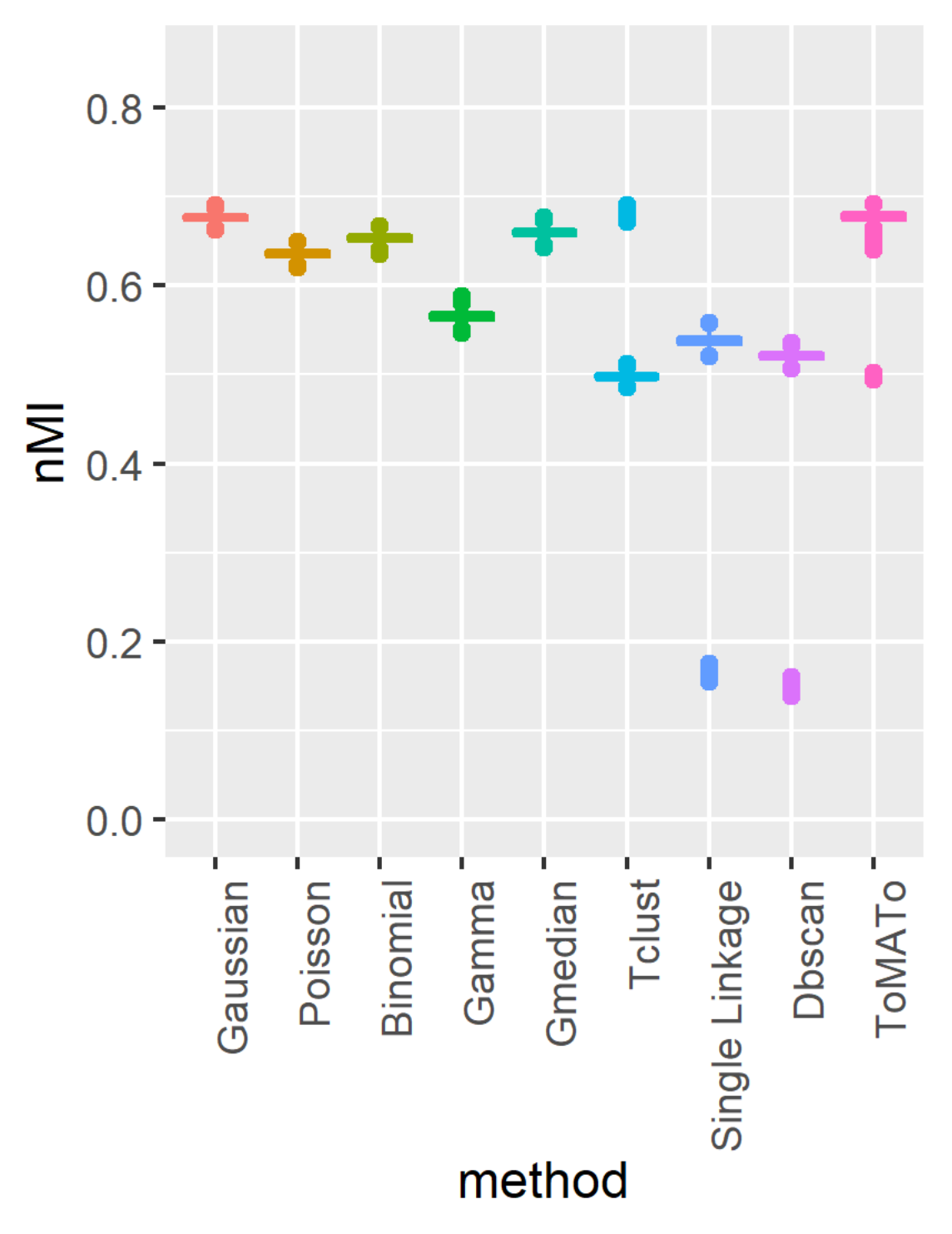
Poisson Refer to caption

Binomial Refer to caption

Gamma Refer to caption

Cauchy Refer to caption

Mixture Refer to caption

Figure 8: NMI for samples of 12000 points

For each clustering procedure, we decide to consider 11000 points as signal. The parameters for the different procedures are the same as described in Section 11.1.1, except for the ToMATo algorithm, we set the parameter m​0=200/12000m0=200/12000. As well, the number of nearest neighbors for the single linkage method is set to 200 and the parameter hh is set to 0.8 for Gaussian distribution, 0.8 for Poisson, 1.1 for Binomial, 0.6 for Gamma, 0.4 for Cauchy and 0.4 for the mixture of 3 different distributions. For dbscan, e​p​seps is the 11000-th smallest distance of a point to its third nearest neighbor.

The NMI over 1000 replications of the experiments are represented via boxplots in Figure 8. Algorithm 1 with the proper Bregman divergence systematically (slightly) outperforms other clustering schemes.

11.2 Discussion about the choice of the Bregman divergence

We consider three mixtures of Gaussian distributions ℒ⁡(c,σ)=13​𝒩​(c1,σ1​I2)+13​𝒩​(c2,σ2​I2)+13​𝒩​(c3,σ3​I2)\mathcal{L}(c,\sigma)=\frac{1}{3}\mathcal{N}(c_{1},\sigma_{1}I_{2})+\frac{1}{3}\mathcal{N}(c_{2},\sigma_{2}I_{2})+\frac{1}{3}\mathcal{N}(c_{3},\sigma_{3}I_{2}) with c=(c1,c2,c3)c=(c_{1},c_{2},c_{3}) for c1=(10,10)c_{1}=(10,10), c2=(25,25)c_{2}=(25,25) and c3=(40,40)c_{3}=(40,40), I2I_{2} the identity matrix on ℝ2\mathbb{R}^{2} and σ=(σ1,σ2,σ3)\sigma=(\sigma_{1},\sigma_{2},\sigma_{3}). The first distribution ℒ1\mathcal{L}_{1} corresponds to clusters with the same variance, with σ=(5,5,5)\sigma=(5,5,5), the second distribution ℒ2\mathcal{L}_{2} to clusters with increasing variance, with σ=(1,4,7)\sigma=(1,4,7), and the third distribution ℒ3\mathcal{L}_{3} to clusters with increasing and decreasing variance, with σ=(2,7,2)\sigma=(2,7,2). We cluster samples of 100 points from ℒ1\mathcal{L}_{1}, ℒ2\mathcal{L}_{2} and then ℒ3\mathcal{L}_{3}. We use Algorithm 1 with the Gaussian, Poisson, Binomial and Gamma Bregman divergences. Note that we set N=50N=50 for the Binomial divergence, so that we expect a clustering with clusters size symmetric with respect to 25. The performance of the clustering in terms of NMI is represented in Figure 9, after 1000 replications of the experiments.

Figure 9: Comparison of Bregman divergences efficiency for different clusters variances.

The corresponding clustering with the best suited Bregman divergence is represented in Figure 10. In particular, we used the Gaussian divergence for ℒ1\mathcal{L}_{1}, the Poisson divergence for ℒ2\mathcal{L}_{2} and the Binomial divergence for ℒ3\mathcal{L}_{3}.

Refer to caption

ℒ1\mathcal{L}_{1} – Gaussian divergence

Refer to caption

ℒ2\mathcal{L}_{2} – Poisson divergence

Refer to caption

ℒ3\mathcal{L}_{3} – Binomial divergence

Figure 10: Clustering with the best suited Bregman divergence

Since the sum of two Bregman divergences is a Bregman divergence, it is also possible to cluster data with Algorithm 1, with a different divergence on the different coordinates. For instance, we sample 100 points from 13​𝒩​(c1,Σ1)+13​𝒩​(c2,Σ2)+13​𝒩​(c3,Σ3)\frac{1}{3}\mathcal{N}(c_{1},\Sigma_{1})+\frac{1}{3}\mathcal{N}(c_{2},\Sigma_{2})+\frac{1}{3}\mathcal{N}(c_{3},\Sigma_{3}), with for every i∈[[1,3]]i\in[\![1,3]\!], Σi\Sigma_{i} diagonal with coefficients (σi(2),σi(3))(\sigma^{(2)}_{i},\sigma^{(3)}_{i}) with σ(2)=(1,4,7)\sigma^{(2)}=(1,4,7) and σ(3)=(2,7,2)\sigma^{(3)}=(2,7,2). In Figure 11, we represented the clustering obtained with Algorithm 1 with the Poisson divergence on the first coordinate and the Binomial divergence on the second coordinate. We observe that the shape of the clusters obtained correspond roughly to the shape of the sublevel sets of the sampling distribution.

Refer to caption
Figure 11: Clustering with hybrid Bregman divergence

11.3 Additional files for Stylometric author clustering

This section exposes the graphics and additional numerics that support several results from Section 4.6, for instance about the calibration of parameters.

Trimmed kk-median:

In Figure 12 we plot the cost and the NMI as a function of qq for different numbers of clusters kk, in Figure 13 we focus on the case k=4k=4. Finally, in Figure 14 we plot the best clusterings in terms of NMI for k=4k=4 and k=6k=6.

Figure 12: Cost and NMI for Author clustering with kk-Median method
Figure 13: Cost and NMI for Author clustering with kk-Median method – k=4k=4
Refer to caption
Refer to caption
Figure 14: Examples of Author clusterings obtained with kk-Median method

These graphics suggest that k=4k=4 and k=6k=6 are possible choices. The corresponding qq that minimize NMI’s are respectively q=202q=202 (N​M​I=0.4334372NMI=0.4334372), and q=208q=208 (N​M​I=0.4721967NMI=0.4721967).

tclust:

Figure 15 and 16 do not allow to select kk. If k=4k=4 is chosen, Figure 16 suggests that q≃184q\simeq 184 is a relevant choice. Figure 17 provides the associated clustering, whose N​M​INMI is 0.49125370.4912537.

Figure 15: Cost and NMI for Author clustering with tclust algorithm
Figure 16: Cost and NMI for Author clustering with tclust algorithm – k=4k=4
Refer to caption
Figure 17: Examples of Author clusterings obtained with tclust algorithm

Trimmed kk-means:

Figure 18 suggests the choice k=4k=4, and Figure 19 shows that q=190q=190 yields a slope jump and NMI peak. The associated clustering is depicted in Figure 20, its NMI is 0.53363080.5336308.

Figure 18: Cost and NMI for Author clustering with trimmed kk-means
Figure 19: Cost and NMI for Author clustering with trimmed kk-means – k=4k=4
Refer to caption
Figure 20: Examples of Author clusterings obtained with trimmed kk-means