Phase-field analysis of quenching and partitioning in a polycrystalline Fe-C system under constrained-carbon equilibrium conditionJournal: Computational Material Science

In the Q&P processing, quenching displacively decomposes austenite to martensite. This diffusionless transformation in a polycrystalline system is simulated by employing an elastic multiphase-field model. Although a comprehensive description of the model is presented elsewhere, Refs. [32, 33], a concise elucidation is rendered in this section.

In a polycrystalline system, the order parameter or phase field, which is introduced in addition to the other thermodynamic variables like concentration and temperature, is treated as an $N$-tuple variable, $\bm{\phi}(\bm{x},t)={(\phi_{1}(\bm{x},t),\phi_{2}(\bm{x},t)....,\phi_{\alpha}(\bm{x},t),\phi_{\beta}(\bm{x},t),...,\phi_{N})}$, where $N$ corresponds to the number of phases or grains in a polycrystalline system, respectively. Furthermore, $\phi_{\alpha}(\bm{x},t)$ is the state variable which assumes $\phi_{\alpha}(\bm{x},t)=1$ in the bulk region $\alpha$ and turns $\phi_{\alpha}(\bm{x},t)=0$ outside. Correspondingly, the phase-field variables represent the volume fraction of the individual phases or grains.

In the phase-field modelling, the transformation is dictated by the phenomenological change in the thermodynamically devised functional. In the present model, a Ginzburg-Landau type free-energy functional $\mathcal{F}(\mbox{{\bm{$\phi$}}},\bm{\nabla}\mbox{{\bm{$\phi$}}},\bar{\mbox{{\bm{$\varepsilon$}}}})$, which consists of interfacial, elastic and chemical contributions, is considered [34]. This free-energy functional is expressed as

where the interfacial free-energy density is the summation of the gradient and the potential energy density, $\bar{W}_{\text{intf}}(\mbox{{\bm{$\phi$}}},\bm{\nabla}\mbox{{\bm{$\phi$}}})=\epsilon a(\bm{\phi},\bm{\nabla}\bm{\phi})+\omega(\bm{\phi})/\epsilon$. The width of the diffuse interface is dictated by the length scale parameter $\varepsilon$. The gradient energy density involved in the interface contribution is expressed as

where $a(\mbox{{\bm{$\phi$}}},\bm{\nabla}\mbox{{\bm{$\phi$}}})$ imparts a form to the interface energy density $\gamma_{\alpha\beta}$, and the normal vector to the $\alpha\beta$-interface is $q_{\alpha\beta}={\phi_{\alpha}\bm{\nabla}{\phi}_{\beta}}-{\phi_{\beta}\bm{\nabla}{\phi}_{\alpha}}$. The potential energy density, formulated as an obstacle-type potential, reads

where the Gibbs simplex $\mathcal{G}=\left\{\bm{\phi}\in\mathbb{R}^{N}:\sum_{\alpha}\phi_{\alpha}=1,\phi_{\alpha}\geq 0\right\}$ assigns sharp minima to the bulk regions of phases, or grains respectively. The higher-order term $\gamma_{\alpha\beta\delta}\phi_{\alpha}\phi_{\beta}\phi_{\delta}$, in Eqn. 3, prevents the formation of non-physical spurious phase-field contributions in binary interface regions. The analytical consistency and computational efficiency of adopting the obstacle-type potential is elucidated in Refs. [35, 36, 37].

The elastic and chemical contribution from the bulk phases are expressed as the interpolation of phase-dependent free-energy densities,

and

From the variation of $\mathcal{F}(\mbox{{\bm{$\phi$}}},\bm{\nabla}\mbox{{\bm{$\phi$}}},\bar{\mbox{{\bm{$\varepsilon$}}}})$, the phase-field evolution is written as

In the above Eqn. 6, $\tilde{N}$ $(\leq N)$ is the number of active phase-fields and $M_{\alpha\beta}$ denotes the mobility of the $\alpha\beta$-interface. Furthermore, the nucleation is modelled through an additional noise term $\zeta$, which is active only in interfacial regions. Since the nucleation of the martensite is not a critical aspect of the present analysis, it is not extensively discussed here. However, the readers are directed to Ref. [33] for a comprehensive understanding on the formulation and consistency of the present nucleation approach.

Apart from the nucleation, the capillarity effect plays a subordinate role in martensite transformation when compared to the chemical and elastic driving forces. Therefore, the stability of the interface is retained through the isotropic gradient energy density term $\epsilon\hat{a}(\phi_{\alpha},\nabla\phi_{\alpha})=-\epsilon\gamma^{c}_{\alpha}\left(\Delta\phi_{\alpha}-|\nabla\phi_{\alpha}|\nabla\cdot\left(\nabla\phi_{\alpha}/|\nabla\phi_{\alpha}|\right)\right),$ which is scaled using an interface parameter, $\gamma^{c}_{\alpha}$ [33]. In Eqn. 6, the variational derivatives of the chemical and elastic driving forces, $\mathopen{}\mathclose{{\left(\delta/\delta\phi_{\beta}-\delta/\delta\phi_{\alpha}}}\right)\mathcal{F}_{\text{chem}}$ and $\mathopen{}\mathclose{{\left(\delta/\delta\phi_{\beta}-\delta/\delta\phi_{\alpha}}}\right)\mathcal{F}_{\text{el}}$, are represented as $\Delta^{\alpha\beta}_{\text{chem}}$ and $\Delta^{\alpha\beta}_{\text{el}}$, respectively. The stresses and driving forces, contributing to the elastic free-energy density, are solved by incorporating the mechanical jump conditions [38, 32].

Using the homogenised normal vector $\bm{n}$, which is determined from the scalar field through

the stresses and strains are expressed in an orthonormal basis $\bm{B}=\{\bm{n},\bm{t},\bm{s}\}$. In the Voigt notation, these stresses and strains are written as

With $\llbracket\cdot\rrbracket^{\alpha\beta}=(\cdot)^{\beta}-(\cdot)^{\alpha}$ representing the jump of the variable across the interface, according to the force balance and the Hadamard kinematic compatibility condition, the jump of $\bm{\sigma}_{n}$ and $\bm{\varepsilon}_{t}$ respectively vanishes ($\llbracket\bm{\sigma}_{n}\rrbracket=\bm{0}$ and $\llbracket\bm{\varepsilon}_{t}\rrbracket=\bm{0}$). Therefore, the continuous contribution of the stresses and strains, for an infinitesimal deformation on a singular plane, can be simplified as $\bm{\sigma}_{n}:={(\sigma_{nn},\sigma_{nt},\sigma_{ns})}$ and $\bm{\varepsilon}_{t}:={(\varepsilon_{tt},\varepsilon_{ss},2\varepsilon_{ts})}$. The discontinuous contributions of the stresses and strains are respectively summarized as $\bm{\sigma}^{\alpha}_{t}:={(\sigma_{tt}^{\alpha},\sigma_{ss}^{\alpha},\sigma_{ts}^{\alpha})}$ and $\bm{\varepsilon}_{n}^{\alpha}:={(\varepsilon_{nn}^{\alpha},2\varepsilon_{nt}^{\alpha},2\varepsilon_{ns}^{\alpha})}$.

The displacement-field gradient, using the Einstein summation convention, is written as $(\nabla\bm{u})_{ij}=\partial u_{i}/\partial x_{j}$. Accordingly, the local strain reads $\bm{\varepsilon}=(\bm{\nabla}\bm{u}+(\bm{\nabla}\bm{u})^{T})/2$.

The stiffness tensor is formulated in the orthonormal basis $\bm{B}$. For the ease of numerical treatment, this tensor is divided into blocks

where $\bm{\mathcal{C}}_{nn}$ and $\bm{\mathcal{C}}_{tt}$ are the symmetrical matrices of dimension $3\times 3$. Furthermore, the $3\times 3$ matrices $\bm{\mathcal{C}}_{nt}$ and $\bm{\mathcal{C}}_{tn}$ satisfy the condition $\bm{\mathcal{C}}_{tn}=\bm{\mathcal{C}}^{\mathsf{\!T}}_{nt}$. The compliance tensor $\bm{\mathcal{S}}^{\alpha}$ is constructed in a similar manner.

By exclusively considering continuous variables, the stresses are calculated by

In Eqn. 15, the normal and tangential components of the inelastic strains $\tilde{\bm{\varepsilon}}^{\alpha}$ are expressed as

respectively. The proportionality matrix, which relates the continuous and discontinuous variables, is locally averaged and is written as

The resulting stresses in the Voigt notations are transformed to the Cartesian coordinate system by $\bm{\bar{\sigma}}^{\text{v}}(\bm{\phi})=\bar{\bm{\mathcal{C}}}^{\text{v}}(\bm{\phi})\bar{\bm{\varepsilon}}^{\text{v}}+\tilde{\bm{\sigma}}^{\text{v}}(\bm{\phi})$, where $\bar{\bm{\mathcal{C}}}^{\text{v}}(\bm{\phi})$ and $\tilde{\bm{\sigma}}^{\text{v}}(\bm{\phi})$ are respectively expressed as $\bar{\bm{\mathcal{C}}}^{\text{v}}(\bm{\phi})=\bm{M}_{\varepsilon}^{\mathsf{\!T}}\bm{\mathcal{C}}^{\text{v}}_{B}(\bm{\phi})\bm{M}_{\varepsilon}$ and $\tilde{\bm{\sigma}}^{\text{v}}(\bm{\phi})=\bm{M}_{\sigma}^{\mathsf{\!T}}\tilde{\bm{\sigma}}_{B}(\bm{\phi})$. The transformation matrices $\bm{M}_{\varepsilon}$ and $\bm{M}_{\sigma}$ are adopted from Ref. [38]. Subsequently, the displacement field $\bm{u}$ is ascertained by solving the momentum balance $\bm{\nabla}\cdot\bar{\bm{\sigma}}(\bm{\phi})=\bm{0}$.

The stresses in the bulk phase ($\alpha$) are calculated by $\sigma_{ij}=(\bm{\mathcal{C}}^{\alpha}[\bm{\varepsilon}-\tilde{\bm{\varepsilon}}^{\alpha}])_{ij}=\mathcal{C}_{ijkl}^{\alpha}(\varepsilon_{kl}-\tilde{\varepsilon}^{\alpha}_{kl}).$ The derivative of the elastic free-energy density reads $\partial\bar{W}_{\text{el}}(\bm{\phi},\bm{\varepsilon}_{B})/\partial\phi_{\alpha}=\partial\sum_{\alpha}p^{\alpha}(\bm{\sigma}_{n},\bm{\varepsilon}_{t})\phi_{\alpha}/\partial\phi_{\alpha}$, wherein $p^{\alpha}(\bm{\sigma}_{n},\bm{\varepsilon}_{t})$ is expressed as

The proportionality matrix $\bm{\mathcal{T}}^{\alpha}$ in Eqn. 20 consists of the components

The consideration that the austenite-martensite $\gamma\alpha^{\prime}$-interface remains stationary during partitioning obviates the need for solving the phase-field evolution equation [9, 15]. Despite this simplification, the partitioning demands a thermodynamically-consistent diffusion of the carbon. Therefore, an established model, based on the grand-potential functional, is involved in the present work to exclusively simulate the partitioning of carbon. With the emphasis to avoid any contribution of the bulk phases to the interface, it has been shown that a more simplistic and a computationally efficient approach can be phenomenologically actualised, if the model is derived from the grand-potential functional with chemical potential as the dynamic variable [39]. An extensive description of present model for a multiphase multicomponent system has already been reported, wherein the sharp-interface solutions are recovered through asymptotic analysis [40, 41]. However, in this section, a brief and a contextual derivation of the phase-field model is extended. Since the current work analyses the evolution in a binary Fe-C system, as opposed to the previous derivations, the concentration and chemical potential are not represented using a vector notation [42, 43, 44]. Moreover, the notations are further simplified by not indicating their dependence of $T$, owing to the isothermal consideration in the present study.

The grand-potential functional, which governs the partitioning of carbon in a domain of volume $V$, is defined as

where $\bar{\Psi}_{\text{bulk}}$ and $\bar{\Psi}_{\text{intf}}$ represent the grand-potential density contribution from the bulk phases and the interfaces, respectively. The interface formulation in the elastic model is adopted here, i.e. $\bar{\Psi}_{\text{intf}}(\mbox{{\bm{$\phi$}}},\bm{\nabla}\mbox{{\bm{$\phi$}}})=\bar{W}_{\text{intf}}(\mbox{{\bm{$\phi$}}},\bm{\nabla}\mbox{{\bm{$\phi$}}})$ in Eqn. 1.

The grand-potential density of the bulk phases are expressed as an interpolation of the grand-potential densities of the individual phases

with $h_{\alpha}\left(\mbox{{\bm{$\phi$}}}\right)$ and $\mu$ representing the interpolation function and the chemical potential, respectively. The grand-potential density of the individual phase $\Psi_{\alpha}$ reads

where $c^{\alpha}$ corresponds to the carbon concentration in $\alpha$. The temporal evolution of the concentration, which dictates the partitioning kinetics, is written as

where $g_{\alpha}(\mbox{{\bm{$\phi$}}})$ interpolates the mobility $\bar{M_{\alpha}}$ [40]. Here, it is important to note that, while $c^{\alpha}$ represents the carbon concentration in $\alpha$, the continuous concentration variable is denoted by $\bar{c}$, which is subsequently introduced in Eqn. 30. Furthermore, the diffusivity $D^{\alpha}(\bar{c})$ in Eqn. 27 not only varies with the phases, but is also influenced by the concentration $\bar{c}$. This influence of concentration on diffusivity is discussed later (Sec. 2.4).

In this formulation, the Legendre transform of the free energy $f_{\alpha}(\bar{c})$, the grand-potential density $\Psi_{\alpha}$, replaces the conventional dynamic variable $\bar{c}$ with the chemical potential $\mu$ and yields the relation

By incorporating Eqn. 25 in the above relation (Eqn. 28), the concentration reads

which can be further simplified to

However, from the above Eqn. 30, the evolution of the concentration is written as

wherein $\dfrac{\partial\bar{c}(\mu,\mbox{{\bm{$\phi$}}})}{\partial\mu}$ and $\dfrac{\partial\bar{c}(\mu,\mbox{{\bm{$\phi$}}})}{\partial t}$ can be expressed as

and

respectively. By rearranging Eqn. 31, and substituting Eqns. 32 and 33, the evolution equation for the chemical potential reads

As elucidated in this section, two distinct functions, $h_{\alpha}\left(\mbox{{\bm{$\phi$}}}\right)$ and $g_{\alpha}\left(\mbox{{\bm{$\phi$}}}\right)$, are conventionally adopted to interpolate the continuous variables across the interface. However, it has recently been shown that the contribution from the bulk and interface can be efficiently decoupled in a chemo-elastic model by interpolating the variables through the phase field [45] In other words, replacing the interpolation functions with the phase field enhances the efficiency of the approach while retaining the thermodynamically consistency. Therefore, in this work, the concentration and the chemical potential are interpolated through the phase-field variable $\phi_{\alpha}$.

Subscribing to the consideration that the carbide formation and the interface migration is precluded during the partitioning of the Q&P treatment, a noticeable deviation from the CALPHAD based equilibrium condition is anticipated. Particularly, the composition of the constituent phases at the end of the partitioning, which directly governs the amount of retained austenite, is assumed to be consistent with the specific equilibrium condition, referred to as constrained carbon equilibrium (CCE). Therefore, by imposing the thermodynamical criterion that the chemical potential of the carbon is equal at the end of the partitioning, the respective concentration of the phases is determined. Correspondingly, equating the activity of carbon yields the relation

where $c^{\gamma}$ and $c^{\alpha^{\prime}}$ represent the respective mole fraction of carbon in austenite and martensite, which is employed for the calculation of the endpoints of the partitioning [46, 47].

The stationary nature of the interface indicates that carbon exclusively diffuses across the interface during the partitioning. Therefore, the number of iron atoms are conserved across the phases, which can be expressed

where $c^{\gamma}_{\text{CCE}}$ and $c^{\text{alloy}}$ represent the mole fraction of carbon after partitioning in austenite and the alloy composition, respectively. Furthermore, while $f^{\gamma}_{\text{CCE}}$ denotes the mole fraction of austenite after partitioning, the initial mole fraction of austenite is given by $f^{\gamma}_{i}$. Although the inequality between $f^{\gamma}_{\text{CCE}}$ and $f^{\gamma}_{i}$ apparently contradicts the assumption of the stationary interface, the negligible change in the volume fraction of the phases, during the extensive diffusion of carbon, accounts for the disparity. From Eqns. 35, 36 and the mass balance relations, expressed as

and

the parameters $c^{\alpha^{\prime}}_{\text{CCE}}$, $c^{\gamma}_{\text{CCE}}$, $f^{\gamma}_{\text{CCE}}$ and $f^{\alpha^{\prime}}_{\text{CCE}}$, which characterize CCE condition, are determined.

As opposed to the conventional incorporation of the CALPHAD data [41], the introduction of the CCE condition demands a certain degree of manipulation. To this end, the martensite is treated as supersaturated ferrite. Moreover, it has been conceded that the CCE condition focuses extensively on establishing the endpoints of the partitioning [4]. Therefore, the numerical manipulation, henceforth presented, is primarily aimed at establishing the characteristic CCE parameters, while being tangible with the CALPHAD data for the chemical driving-force.

In the binary Fe-C system, owing to the interstitial occupation of the carbon atoms, the free energy of a given phase $\Theta$, which can be $\gamma$ or $\alpha^{\prime}$, is expressed as

In this formulation, the dependence of the free energy on the concentration is expressed in terms of the site fraction $Y_{i}^{s}$, where $s$ denotes the sub-lattices ($1$ or $2$) and $i$ represents the component occupying the sub-lattice. The sub-lattice 1 is occupied by iron ($Fe$) and a fraction of the sub-lattice $2$ is occupied by carbon ($C$), based on the carbon concentration, leaving the remaining sites vacant ($Va$). The site-fraction is related to the mole fraction through the expression $c_{i}=\frac{{\underset{s}{\sum}}a^{s}Y_{i}^{s}}{{\underset{s}{\sum}}a^{s}(1-Y_{Va}^{s})}$, where $a^{s}$ is the number of sites in the sub-lattice $s$ per unit mole. Moreover, $f_{Fe:Va}$ and $f_{Fe:C}$ correspond to the free energy of pure iron and Fe-C steel, respectively. The constant $\tilde{a^{2}}$ varies with the crystal structure of the phases. For ferrite $\tilde{a^{2}}=3$, while for austenite $\tilde{a^{2}}=1$. $\bar{L}_{Fe:Va,C}$ denotes the interaction parameter with comma and colon separating the components and the sub-lattices, respectively. The extensive formulation of the free energy in Eqn. 39 can be simplified using mole fraction [45] and written as

Correspondingly, the first and second derivatives of the free energy are expressed as

and

where $V_{\text{m}}$ corresponds to the molar volume of the phases and $G^{\Theta}$ is the Gibbs free-energy which the CALPHAD database renders [48]. Though, the numerical co-coefficients $A^{\Theta}$, $B^{\Theta}$ and $D^{\Theta}$ do not posses any thermodynamic significance, a proper fitting facilitates the replication of the CALPHAD based free-energy plot through these parameters [45]. Furthermore, by appropriately manipulating these co-coefficients the CCE condition can be introduced into the simulation.

The numerical approach, which relates the co-coefficients with the CALPHAD data, begins by defining a concentration-step of finite magnitude, $\Delta c$ [41]. The Gibbs free-energy at a specific composition, which is considered to be the equilibrium composition ($c_{\text{eq}}$) here, and the neighbouring compositions defined by $\Delta c$ are determined from the database. Thus, the free energies $G^{\Theta}_{c_{\text{eq}}}$, $G^{\Theta}_{c_{\text{eq}}^{1}}$, $G^{\Theta}_{c_{\text{eq}}^{2}}$, $G^{\Theta}_{\tilde{{c_{\text{eq}}^{1}}}}$ and $G^{\Theta}_{\tilde{{c_{\text{eq}}^{2}}}}$ correspond to the composition $c_{\text{eq}}$, $c_{\text{eq}}+\Delta c$, $c_{\text{eq}}+2\Delta c$, $c_{\text{eq}}-\Delta c$ and $c_{\text{eq}}-2\Delta c$, respectively. An ‘environment ’ surrounding the equilibrium composition is re-created around the predetermined $c_{\text{CCE}}$ through the following consideration

and

wherein $G^{\Theta}_{c_{\text{CCE}}}$, the free energy of the phases at $c^{\Theta}_{\text{CCE}}$ is obtained from the CALPHAD database.

If $A^{\Theta}_{\text{CCE}}$, $B^{\Theta}_{\text{CCE}}$ and $D^{\Theta}_{\text{CCE}}$ are the modified co-coefficients which introduce the CCE conditions, the adapted free energy is represented by

By substituting Eqns 43-46 and adopting a five-point stencil scheme in finite-difference approximation [41, 45], the co-coefficients are determined by

and

Furthermore, the condition

is invoked in the Newton-Raphson iteration technique, to ensure that the modified free-energy formulation (Eqn. 47) yields equal chemical potential at the compositions $c^{\gamma}_{\text{CCE}}$ and $c^{\alpha^{\prime}}_{\text{CCE}}$. The thermodynamic data for the stoichiometric compounds are introduced by numerically fitting a sharp curve with its minima at the point rendered by the CALPHAD data [41]. Although the present approach is motivated by this methodology of introducing the stoichiometric compounds, the $\Delta c$ is appropriately chosen such that through Eqns 43-46 a tangibility with the CALPHAD data is attained.

The kinetics of the carbon diffusion, during the partitioning, is governed by its diffusivity in the corresponding phases. To encompass the influence of the carbon concentration on the diffusivity, the following formulations,

and

are incorporated in the model to account for the diffusion constant in austenite ($D^{\gamma}(c)$) and martensite ($D^{\alpha^{\prime}}$), respectively [49, 50, 51]. In Eqn. 51, the carbon concentration is incorporated as $y_{c}=c/(1-c)$. Owing to the difference in the diffusivities, it is shown that the carbon accumulates in the $\gamma\alpha^{\prime}$-interface during the partitioning [15, 30]. From Eqn. 51, it is conceivable that the accumulation of the carbon, particularly under CCE conditions, increases the diffusivity in austenite beyond $D^{\alpha^{\prime}}$. To preclude such nonphysical changes in the diffusivities, a cut-off is defined, which ensures that a minimum difference in the diffusion constants is retained at $10^{-3}$ at any stage of the transformation [31].

The 2-dimensional domain, considered in the present work, is spatially discretised through the finite-difference approach. This discretisation decomposes the domain into uniform grids of dimension $\Delta\text{x}=\Delta\text{y}=0.05\penalty\ \upmu\text{m}$. The domain size of dimension 800 $\times$ 800 cells, rendering 40 $\upmu$m $\times$ 40 $\upmu$m domain, is considered for all simulations. The evolution equations formulated in Sec. 2.1 and Sec. 2.2 are solved on the grid points using finite-difference algorithm with an explicit forward Euler scheme. The length parameter $\varepsilon$, which dictates the width of the diffuse interface, is fixed at $2.5\penalty\ \Delta\text{x}$ [40].

The numerical efficiency of the present approach is enhanced by incorporating the models to the in-house software package Pace3D (Parallel Algorithms for Crystal Evolution in 3D). Furthermore, the consumption of the computational resources is optimised through the domain decomposition using Message Passing Interface (MPI). The polycrystalline set-up is achieved through the Voronoi tessellation which yields 200 grains [52, 53]. In order to achieve a time-invariant normal distribution of the grains, which are devoid of any artifacts, the microstructure is allowed to evolve in an isotropic condition, till the total number of grains is reduced to 100.

The volume fraction of martensite ($f^{\alpha^{\prime}}$), which results from quenching, influences the amount of retained austenite both directly and indirectly. In a two phase system of martensite and austenite, $f^{\alpha^{\prime}}$ ascertains the amount of austenite available for any transformations. Furthermore, since the endpoints of the partitioning vary with the martensite volume-fraction, Eqns. 35- 38, $f^{\alpha^{\prime}}$ indirectly influences the amount of retained austenite.

To simulate a definite volume fraction of martensite, an Fe-C system with carbon concentration $c=0.009$ ($\text{C}=0.2\penalty\ \text{wt}\%$) is considered. The quenching temperature which yields the desired martensite volume-fraction is calculated from the Koistinen-Marburger equation [16]. This relation between the volume fraction $f^{\alpha^{\prime}}$ and temperature ($T$) is expressed as

where $M_{\text{s}}$ is the martensite start temperature. The $M_{\text{s}}$ temperature varies with the carbon content. From Ref. [54], $M_{\text{s}}$ temperature for a given concentration is calculated by

where $\alpha_{m}$, in Eqn. 53, is the rate parameter which is written as

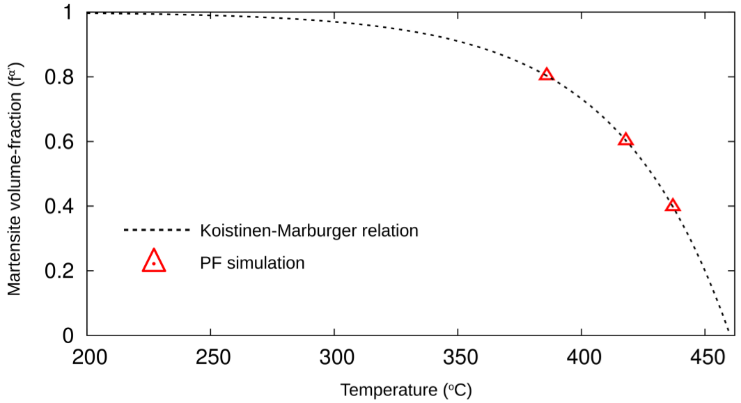
In the aforementioned Eqns. 53- 55, the concentration C is the weight percent of carbon, while the temperatures ($T$ and $M_{\text{s}}$) are considered in $\degree\text{C}$. Three different volume fractions of martensite are arbitrarily chosen: $f^{\alpha^{\prime}}$= 0.4, 0.6 and 0.8, and the corresponding quenching temperatures are determined from Eqn. 53. The chemical driving-forces pertaining to the quenching temperatures, which are deduced from the CALPHAD database, are presented in Table 1.

The diffusionless transformation of martensite is accompanied by the change in the crystal structure from Face-Centered Cubic (FCC-austenite) to Body-Centered Tetragonal (BCT-martensite). The transition in the crystal structure introduces strain owing to the difference in the lattice parameters. This strain, which is induced despite the absence of any external stresses, is conventionally referred to as stress-free transformation strain or eigenstrain. In the present work, the eigenstrains are introduced as phase-dependent Bain strains which are written as

The eigenstrains $\varepsilon_{1}$ and $\varepsilon_{3}$ which dictate the Bain strains are calculated from the crystal lattice parameter. The formulation used for determining the lattice parameter and its other implications in the present work are consolidated in the Appendix. Since the grains in a polycrystalline microstructure are rotated randomly, the eigenstrains are correspondingly rotated through the rotation matrix $Q$, in the $z-y^{\prime}-x^{\prime\prime}$ intrinsic rotation convention. Therefore, the elastic strains become $\tilde{\varepsilon}^{00}_{ij}=Q_{im}Q_{jn}\tilde{\varepsilon}^{000}_{mn}$, depending on the crystal orientation of the grain. Furthermore, the misfit strain relaxation at austenite grain boundaries [55] is included by

where the factor $0\leq\rho\leq 1$ determines the strength of the relaxation. In Eqn. 57, $\phi_{\alpha}^{t_{0}}$ and $\phi_{\beta}^{t_{0}}$ are the phase-field variables which are assigned once the diffuse interface is established between the grains (at time $t=0$). The misfit strain relaxation is accommodated in the eigenstrain matrix by $\tilde{\bm{\varepsilon}}^{0}=\Gamma(\bm{\phi}^{t_{0}})\tilde{\bm{\varepsilon}}^{00}$.

Although the Bain strains, which govern the martensite evolution, account for the elastic strains, experimental investigations indicate that the displacive transformation is additionally accompanied by plastic strains [56]. Since plasticity is not included in the current phase-field model, the components of the Bain strains are reduced by a prefactor $f_{\text{c}}$, which transforms the eigenstrains to $\varepsilon_{1}=\varepsilon_{1}^{0}f_{\text{c}}$ and $\varepsilon_{3}=\varepsilon_{3}^{0}f_{\text{c}}$. The prefactor avoids unphysically high elastic driving-forces [57]. The different prefactors, $f_{\text{c}}$, which vary with the temperature, are presented in Table 1. The material parameters, encompassing both elastic and interface parameter, which are incorporated in the model are tabulated in Table 2.

Since the martensite exhibits a rapid transformation rate, a refined time-step $\Delta t$ with no physical significance is considered, despite the consideration of the quantitative driving force. For all simulations, the noise term in Eq. 6 is applied every hundredth time step with a uniform distribution which is scaled to result in a fluctuation up to 0.2 in the phase fields. In the first time step, a three-fold higher noise is employed to stimulate first-time nucleation. It should be pointed out a noise of phase $\alpha$ is only activated in its respective parental grain.

The microstructural changes accompanying the diffusionless transformation of austenite in a polycrystalline set-up are presented in Fig. 2(a). Furthermore, the corresponding evolution of the von Mises stress ($\sigma_{\text{mises}}$), which signifies the accumulation of the elastic energy, is included. In the initial stages of the transformation, at $t=1200\Delta t$, it is evident that the mechanical strains are established during the displacive decomposition of austenite. However, since the chemical driving-force at these early stages are exceedingly high, compared to the mechanical forces, the martensite grows despite the build-up of the stress. As shown in Fig. 2(a) at $t=4000\Delta t$, with an increase in the volume fraction (size) of the martensite, the elastic strains increase visibly. Consequently, the elastic energy becomes comparable to the chemical driving-force and decreases the rate of the transformation considerably. When the mechanical stress, developed during the diffusionless decomposition, matches the chemical driving force, the transformation halts ($t=10000\Delta t$). This balance between the chemical and mechanical (elastic) forces yields a definite volume fraction of martensite. The amount of martensite emerging from the displacive transformation of the austenite is ascertained for the different temperatures considered in Table 1. The martensite volume-fractions are plotted along with the Koistinen-Marburger equation in Fig. 2(b). This representation reveals a noticeable agreement between the fraction of the decomposed austenite and the analytical prediction.

References

- [1] H.K.D.H. Bhadeshia and D.V. Edmonds. Tempered martensite embrittlement: Role of retained austenite and cemenite. Met. Sci., 13(6):325–334, 1979.
- [2] Y. Ojima, Y. Shiroi, Y. Taniguchi, and K. Kato. Application to body parts of high-strength steel sheet containing large volume fraction of retained austenite. Technical report, SAE Technical Paper, 1998.
- [3] G. Thomas. Retained austenite and tempered martensite embrittlement. Metallurgical Transactions A, 9(3):439–450, 1978.
- [4] J. Speer, D.K. Matlock, B.C. De Cooman, and J.G. Schroth. Carbon partitioning into austenite after martensite transformation. Acta materialia, 51(9):2611–2622, 2003.
- [5] J.G. Speer, D.V. Edmonds, F.C. Rizzo, and D.K. Matlock. Partitioning of carbon from supersaturated plates of ferrite, with application to steel processing and fundamentals of the bainite transformation. Current Opinion in Solid State and Materials Science, 8(3-4):219–237, 2004.
- [6] D.K. Matlock, V.E. Brautigam, and J.G. Speer. Application of the quenching and partitioning (q&p) process to a medium-carbon, high-si microalloyed bar steel. In Materials Science Forum, volume 426, pages 1089–1094. Trans Tech Publications Ltd., Zurich-Uetikon, Switzerland, 2003.
- [7] M.J. Santofimia, L. Zhao, and J. Sietsma. Microstructural evolution of a low-carbon steel during application of quenching and partitioning heat treatments after partial austenitization. Metallurgical and Materials Transactions A, 40(1):46, 2009.
- [8] M.J. Santofimia, L. Zhao, and J. Sietsma. Overview of mechanisms involved during the quenching and partitioning process in steels. Metallurgical and Materials Transactions A, 42(12):3620, 2011.
- [9] Y. Toji, H. Matsuda, M. Herbig, P.-P. Choi, and D. Raabe. Atomic-scale analysis of carbon partitioning between martensite and austenite by atom probe tomography and correlative transmission electron microscopy. Acta Materialia, 65:215–228, 2014.
- [10] M. Hillert and J. Agren. On the definitions of paraequilibrium and orthoequilibrium. Scripta Materialia, 50(5):697–699, 2004.
- [11] A.J. Clarke, J.G. Speer, M.K. Miller, R.E. Hackenberg, D.V. Edmonds, D.K. Matlock, F.C. Rizzo, K.D. Clarke, and E. De Moor. Carbon partitioning to austenite from martensite or bainite during the quench and partition (q&p) process: A critical assessment. Acta materialia, 56(1):16–22, 2008.
- [12] J.G. Speer, E. De Moor, and A.J. Clarke. Critical assessment 7: quenching and partitioning. Materials Science and Technology, 31(1):3–9, 2015.
- [13] T.D. Bigg, D.V. Edmonds, and E.S. Eardley. Real-time structural analysis of quenching and partitioning (q&p) in an experimental martensitic steel. Journal of Alloys and Compounds, 577:S695–S698, 2013.
- [14] T.D. Bigg, D.K. Matlock, J.G. Speer, and D. Edmonds. Dynamics of the quenching and partitioning (q&p) process. In Solid State Phenomena, volume 172, pages 827–832. Trans Tech Publ, 2011.
- [15] Y. Toji, G. Miyamoto, and D. Raabe. Carbon partitioning during quenching and partitioning heat treatment accompanied by carbide precipitation. Acta Materialia, 86:137–147, 2015.
- [16] D.P. Koistinen and R.E. Marburger. A general equation prescribing the extent of the austenite-martensite transformation in pure iron-carbon alloys and plain carbon steels. acta metallurgica, 7(1):59–60, 1959.
- [17] A.J. Clarke, J.G. Speer, D.K. Matlock, F.C. Rizzo, D.V. Edmonds, and M.J. Santofimia. Influence of carbon partitioning kinetics on final austenite fraction during quenching and partitioning. Scripta Materialia, 61(2):149–152, 2009.
- [18] M.J. Santofimia, J.G. Speer, A.J. Clarke, L. Zhao, and J. Sietsma. Influence of interface mobility on the evolution of austenite–martensite grain assemblies during annealing. Acta Materialia, 57(15):4548–4557, 2009.
- [19] N. Zhong, X. Wang, Y. Rong, and L. Wang. Interface migration between martensite and austenite during quenching and partitioning (q&p) process. Journal of Materials Science & Technology, 22(6):751–754, 2006.
- [20] J.G. Speer, R.E. Hackenberg, B.C. Decooman, and D.K. Matlock. Influence of interface migration during annealing of martensite/austenite mixtures. Philosophical magazine letters, 87(6):379–382, 2007.
- [21] M.J. Santofimia, L. Zhao, and J. Sietsma. Model for the interaction between interface migration and carbon diffusion during annealing of martensite–austenite microstructures in steels. Scripta Materialia, 59(2):159–162, 2008.
- [22] L.-Q. Chen. Phase-field models for microstructure evolution. Annual review of materials research, 32(1):113–140, 2002.
- [23] I. Steinbach. Phase-field model for microstructure evolution at the mesoscopic scale. Annual Review of Materials Research, 43:89–107, 2013.
- [24] Ramanathan Perumal, PG Kubendran Amos, Michael Selzer, and Britta Nestler. Phase-field study on the formation of first-neighbour topological clusters during the isotropic grain growth. Computational Materials Science, 140:209–223, 2017.
- [25] P.G. Kubendran Amos, L.T. Mushongera, T. Mittnacht, and B. Nestler. Phase-field analysis of volume-diffusion controlled shape-instabilities in metallic systems-ii: Finite 3-dimensional rods. Computational Materials Science, 144:374–385, 2018.
- [26] Tobias Mittnacht, PG Kubendran Amos, Daniel Schneider, and Britta Nestler. Understanding the influence of neighbours on the spheroidization of finite 3-dimensional rods in a lamellar arrangement: Insights from phase-field simulations. In Numerical Modelling in Engineering, pages 290–299. Springer, 2018.
- [27] G Caginalp. Stefan and hele-shaw type models as asymptotic limits of the phase-field equations. Physical Review A, 39(11):5887, 1989.
- [28] H. Garcke, B. Nestler, and B. Stoth. On anisotropic order parameter models for multi-phase systems and their sharp interface limits. Physica D: Nonlinear Phenomena, 115(1-2):87–108, 1998.
- [29] I. Steinbach, B. Böttger, J. Eiken, N. Warnken, and S.G. Fries. Calphad and phase-field modeling: a successful liaison. Journal of phase equilibria and diffusion, 28(1):101–106, 2007.
- [30] Y. Takahama, M.J. Santofimia, M.G. Mecozzi, L. Zhao, and J. Sietsma. Phase field simulation of the carbon redistribution during the quenching and partitioning process in a low-carbon steel. Acta Materialia, 60(6-7):2916–2926, 2012.
- [31] M.G. Mecozzi, J. Eiken, M.J. Santofimia, and J. Sietsma. Phase field modelling of microstructural evolution during the quenching and partitioning treatment in low-alloy steels. Computational Materials Science, 112:245–256, 2016.
- [32] D. Schneider, E. Schoof, O. Tschukin, A. Reiter, C. Herrmann, F. Schwab, M. Selzer, and B. Nestler. Small strain multiphase-field model accounting for configurational forces and mechanical jump conditions. Computational Mechanics, pages 1–19, 2017.
- [33] E. Schoof, D. Schneider, N. Streichhan, T. Mittnacht, M. Selzer, and B. Nestler. Multiphase-field modeling of martensitic phase transformation in a dual-phase microstructure. International Journal of Solids and Structures, 134:181–194, 2018.
- [34] V.I. Ginzburg. On the theory of superconductivity. Zh. eksper. teor. Fiz., 20:1064–1082, 1950.
- [35] H. Garcke, B. Nestler, and B. Stoth. A multiphase field concept: numerical simulations of moving phase boundaries and multiple junctions. SIAM Journal on Applied Mathematics, 60(1):295–315, 1999.
- [36] Y. Oono and S. Puri. Study of phase-separation dynamics by use of cell dynamical systems. i. modeling. Physical Review A, 38(1):434, 1988.
- [37] J. Hötzer, O. Tschukin, M. Ben Ben Said, M. Berghoff, M. Jainta, G. Barthelemy, N. Smorchkov, D. Schneider, M. Selzer, and B. Nestler. Calibration of a multi-phase field model with quantitative angle measurement. Journal of materials science, 51(4):1788–1797, 2016.
- [38] D. Schneider, O. Tschukin, A. Choudhury, M. Selzer, T. Böhlke, and B. Nestler. Phase-field elasticity model based on mechanical jump conditions. Computational Mechanics, 55(5):887–901, 2015.
- [39] M. Plapp. Unified derivation of phase-field models for alloy solidification from a grand-potential functional. Physical Review E, 84(3):031601, 2011.
- [40] A. Choudhury and B. Nestler. Grand-potential formulation for multicomponent phase transformations combined with thin-interface asymptotics of the double-obstacle potential. Physical Review E, 85(2):021602, 2012.
- [41] P.G. Kubendran Amos, L.T. Mushongera, and B. Nestler. Phase-field analysis of volume-diffusion controlled shape-instabilities in metallic systems-i: 2-dimensional plate-like structures. Computational Materials Science, 144:363–373, 2018.
- [42] PG Kubendran Amos, Avisor Bhattacharya, Britta Nestler, and Kumar Ankit. Mechanisms of pearlite spheroidization: Insights from 3d phase-field simulations. Acta Materialia, 161:400–411, 2018.
- [43] P.G. Kubendran Amos, E. Schoof, D. Schneider, and B. Nestler. On the globularization of the shapes associated with alpha-precipitate of two phase titanium alloys: Insights from phase-field simulations. Acta Materialia, 159:51–64, 2018.
- [44] PG Kubendran Amos, Ephraim Schoof, Daniel Schneider, and Britta Nestler. On the volume-diffusion governed termination-migration assisted globularization in two-phase solid-state systems: Insights from phase-field simulations. In Numerical Modelling in Engineering, pages 47–63. Springer, 2018.
- [45] P.G. Kubendran Amos, E. Schoof, D. Schneider, and B. Nestler. Chemo-elastic phase-field simulation of the cooperative growth of mutually-accommodating widmanstätten plates. Journal of Alloys and Compounds, 767:1141–1154, 2018.
- [46] Joseph A Lobo and Gordon H Geiger. Thermodynamics and solubility of carbon in ferrite and ferritic fe-mo alloys. Metallurgical Transactions A, 7(8):1347–1357, 1976.
- [47] Joseph A Lobo and Gordon H Geiger. Thermodynamics of carbon in austenite and fe-mo austenite. Metallurgical Transactions A, 7(8):1359–1364, 1976.
- [48] P. Gustafson. A thermodynamic evaluation of the fe–c system. Scand. J. Metall., 14(5):259–267, 1985.
- [49] J. Agren. Computer simulations of the austenite/ferrite diffusional transformations in low alloyed steels. Acta Metallurgica, 30(4):841–851, 1982.
- [50] J. Agren. A revised expression for the diffusivity of carbon in binary fe-c austenite. Scripta metallurgica, 20(11):1507–1510, 1986.
- [51] E.J. Seo, L. Cho, and B.C. De Cooman. Kinetics of the partitioning of carbon and substitutional alloying elements during quenching and partitioning (q&p) processing of medium mn steel. Acta Materialia, 107:354–365, 2016.
- [52] F. Aurenhammer. Voronoi diagrams—a survey of a fundamental geometric data structure. ACM Computing Surveys (CSUR), 23(3):345–405, 1991.
- [53] R. Perumal, P.G. Kubendran Amos, M. Selzer, and B. Nestler. Phase-field study of the transient phenomena induced by’abnormally’large grains during 2-dimensional isotropic grain growth. COMPUTATIONAL MATERIALS SCIENCE, 147:227–237, 2018.
- [54] S.M.C. Van Bohemen. Bainite and martensite start temperature calculated with exponential carbon dependence. Materials Science and Technology, 28(4):487–495, 2012.
- [55] T.W. Heo and L.-Q. Chen. Phase-field modeling of displacive phase transformations in elastically anisotropic and inhomogeneous polycrystals. Acta Materialia, 76:68–81, 2014.
- [56] G. Krauss. Martensite in steel: strength and structure. Materials science and engineering: A, 273:40–57, 1999.
- [57] C. Hüter, M. Lin, D. Schicchi, M. Hunkel, U. Prahl, and R. Spatschek. A multiscale perspective on the kinetics of solid state transformations with application to bainite formation. AIMS Materials Science, 2(4):319–345, 2015.
- [58] S. Samanta, S. Das, D. Chakrabarti, I. Samajdar, S.B. Singh, and A. Haldar. Development of multiphase microstructure with bainite, martensite, and retained austenite in a co-containing steel through quenching and partitioning (q&p) treatment. Metallurgical and Materials Transactions A, 44(13):5653–5664, 2013.
- [59] J. Hötzer, M. Jainta, P. Steinmetz, B. Nestler, A. Dennstedt, A. Genau, M. Bauer, H. Köstler, and U. Rüde. Large scale phase-field simulations of directional ternary eutectic solidification. Acta Materialia, 93:194–204, 2015.
- [60] L.T. Mushongera, P.G. Kubendran Amos, B. Nestler, and K. Ankit. Phase-field simulations of pearlitic divergence in fe-c-mn steels. Acta Materialia, 150:78–87, 2018.
- [61] N.N. Rammo and O.G. Abdulah. A model for the prediction of lattice parameters of iron–carbon austenite and martensite. Journal of alloys and compounds, 420(1-2):117–120, 2006.