Single-shot quantum memory advantage in the simulation of stochastic processes
Stochastic processes underlie a vast range of natural and social phenomena Book-Duan2015; Book-Jacobs2010. Some processes such as atomic decay feature intrinsic randomness, whereas other complex processes, e.g. traffic congestion, are effectively probabilistic because we cannot track all relevant variables. To simulate a stochastic system’s future behaviour, information about its past must be stored Crutchfield1989; Shalizi2001and thus memory is a key resource. Quantum information processing promises a memory advantage for stochastic simulation Gu2012; Mahoney2016; Riechers2016; Cabello2016; Thompson2017; Suen2017; Elliott2018; Aghamohammadi2018; Cabello2018; Binder2018; Thompson2018 that has been validated in recent proof-of-concept experiments Palsson2017; Ghafari2017. Yet, in all past works, the memory saving would only become accessible in the limit of a large number of parallel simulations Schumacher1995; Mahoney2016, because the memory registers of individual quantum simulators had the same dimensionality as their classical counterparts. Here, we report the first experimental demonstration that a quantum stochastic simulator can encode the relevant information in fewer dimensions than any classical simulator, thereby achieving a quantum memory advantage even for an individual simulator. Our photonic experiment thus establishes the potential of a new, practical resource saving in the simulation of complex systems.
Here we realise the first experimental demonstration of a single-shot memory advantage for simulating stochastic processes. By “single-shot” we mean that any individual simulator obtains an advantage, rather than requiring an asymptotically large array of simulators. We investigate a specific stochastic process, while noting that it is theoretically known that the advantage holds for a range of other simulation tasksBinder2018. The process we simulate here can be understood as the output of a biased perturbed coin after post-processing Thompson2018(see Fig. 1a): at each discrete time step, the state of the coin provides a probabilistic binary outcome, which depends on the parameters and that are defined by the process. Over multiple time steps, this produces a string of ‘zero’s and ‘one’s. Then, in post-processing, every ‘0’ that precedes a ‘1’ is replaced by a ‘2’. For classical simulation, this post-processing markedly increases the amount of past information that needs to be stored in order to generate future predictions. This is not so for quantum processors.
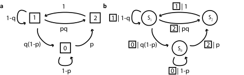
It is known that for the provably optimal simulators Thompson2018 in each class (classical or quantum) of this stochastic process (Fig. 1b), it suffices to classify any possible past into three different states called causal states Shalizi2001; Gu2012. To this end, the classical processor must have three distinguishable states, , as its memory. By contrast, as we experimentally demonstrate, the quantum processor works with the three required quantum states, , compressed into a two-dimensional quantum system.
Generally, as illustrated in Fig. 2a, a quantum simulator of a stochastic process, henceforth simply referred to as a quantum simulator, accepts a memory system and an ancilla system as inputs to a unitary transformation Gu2012; Mahoney2016; Binder2018 for each simulation step. Of the two, only the memory system contains information about the past, while the ancilla system carries no information. The unitary transformation produces an entangled state of the output memory system and a second system. Measurement of the latter provides the output of the stochastic process, and collapses the memory system to the appropriate quantum state for the next simulation step. Importantly, the memory register enters and exits the quantum processor (W) as a two-dimensional system, unlike its classical counterpart in Fig. 2b, where the memory register is a three-dimensional system.

For the stochastic process of Fig. 1, the quantum memory required is a single qubit, in which the three causal states are encoded as three, non-mutually-orthogonal, pure quantum states, as described in Methods. We implement our simulator in a photonic quantum information processor. The memory qubit is encoded in the polarisation degree of freedom of a single photon. The non-trivial unitary transformations in our experiment include a mapping from the memory qubit to a qutrit space of three spatial modes (paths), followed by a controlled-NOT (C-NOT) O'Brien2003; Langford2005 and a controlled-rotation (C-rotation) gate, as detailed in Fig. 2c. The path measurement of this photon corresponds to measuring the qutrit in the logical basis, which provides the classical output (0, 1 or 2) of that step of the stochastic process. This collapses the output memory qubit, encoded in the polarisation state of another photon, to the correct conditional state, which can be characterised by quantum state tomography.
We overcome constraints in the nondeterministic photonic implementation of consecutive quantum gates by introducing a non-destructive measurement realised by an additional C-NOT gate Pryde2004; Ralph2006 and a corresponding ancilla photon. The photons are generated via spontaneous parametric downconversion (SPDC) and four-fold coincidences (three photons for the experiment and one “spare” photon to herald the presence of its pair) are detected using superconducting nanowire single-photon detectors (SNSPDs Baek2011) and coincidence logic modules. The detailed experimental setup is shown in Fig 3, and additional details are in Methods.
The first goal of the experiment is to verify that the quantum simulator is performing the intended simulation. For this, two criteria must be fulfilled: i) After initialisation in each of the three possible causal states, the conditional output statistics, obtained through the qutrit measurement, should match the transition probabilities that determine the stochastic process (see Fig. 1). ii) Conditioned on the qutrit measurement outcome, the correct memory state should be produced, to allow the possibility of further simulation steps.

To check the first criterion, we prepare each of the three causal states, whose definitions in terms of and are provided in the Methods section. For each input causal state there is a probability distribution over the three possible outputs of the stochastic process. Comparing the measured distributions with the theoretical ones, we consistently obtain (classical) fidelities Book-Nielsen2010 above . For the second criterion, the collapsed output memory state is reconstructed by quantum state tomography, given each of the input causal states. The (quantum) fidelities of our experimental stationary states (see Methods) with the ideal stationary states are all above .
The second goal of the experiment is to demonstrate the quantum advantage in memory requirements. A stochastic simulator can be used in different ways, with correspondingly different ways of analysing the memory use. The most straightforward use is as a single simulator. In this scenario, the memory size, in bits, is measured by the max-entropy, which is simply , where is the dimensionality of the memory system Schumacher1995; Mahoney2016. Since the information about the past is encoded in the polarisation of a single photon, both at the beginning and at the end of the simulated step, the memory system that connects steps is obviously confined to a qubit space. In contrast to this two-level quantum system, the optimal classical simulator requires a three-level systemThompson2018. Thus, there is a clear single-shot quantum advantage in memory.
If multiple simulations are run in parallel, the required memory is no longer determined by the dimensionality of the memory system alone. In the limit of a very large number () of parallel simulations (the independent and identically distributed (i.i.d.) case Schumacher1995; Mahoney2016), the minimum required memory to replicate the process faithfully is given by , where is called the statistical complexity Crutchfield1989. The classical statistical complexity Crutchfield1989, , is the Shannon entropy of the stationary distribution over causal states, while the quantum statistical complexity Gu2012, , is the von Neumann entropy of the quantum stationary state (see Methods for mathematical definitions).
Fig. 4a illustrates the theoretically-expected statistical complexities and for all possible values of and , showing the potential for a significant quantum advantage over a large region of the parameter space. We perform the simulation for sets of values along several cross-sections. The experimental values of , shown in Fig. 4b-e, are determined from the density matrices of the output memory system and the transition probabilities (see Methods). The slight deviations of the experimental data compared to the theoretical curves arises from experimental imperfections such as reduced qubit purity from imperfect nonclassical interference, small imperfections and setting errors in polarisation-dependent elements, and a minor imbalance in detector efficiencies. These results nevertheless demonstrate a substantial quantum advantage in the required memory for simulation in the i.i.d. case.

Thus, our quantum simulator has an advantage over its classical counterpart both for the single-shot and i.i.d. cases. Remarkably, we even simulate processes, marked by the shaded regions in Fig. 4b-e, where the classical statistical complexity exceeds one bit. In these cases, we have a gap between both quantum measures and both classical measures: . (Note that always forms an upper bound on the Shannon or von Neumann entropy.)
The present experiment allows us to study both the statistical complexity and the dimensionality of the memory system. However, for more complex processes that entail high-dimensional memory systems, the quantum state tomography required for the estimation of the statistical complexity would require increased resources (such as photons, modes, detectors), and could become prohibitively time-consuming. In contrast, verifying a dimensionality advantage remains straightforward, because it is based on counting dimensions of a Hilbert space rather than characterising quantum states. We perform a single step of the simulation in our experiment, which is already sufficient for demonstrating a quantum advantage. In the future, it would be interesting to perform multiple simulation steps with a single-shot quantum advantage.
A natural question is to ask: what is the prevalence of such dimensionality advantage? While this remains an open question, its existence is certainly not isolated to the stochastic process in this experiment. Indeed, such advantage arises naturally in the context of processes that exhibit causal asymmetry—a memory overhead (in both dimensional and entropic memory costs) between predicting the future versus retrodicting the past Crutchfield2009. All such processes lead to dimensionality advantage, and there exist families of processes where this advantage can grow without bound Thompson2018.
In conclusion, we have shown that quantum information processing enables the simulation of a stochastic process with a memory that is smaller both in terms of its dimensionality (the number of orthogonal states it can support) and its von Neumann entropy, compared to the optimal classical simulator, measured by the number of states it uses and the Shannon entropy, respectively. The demonstrated decrease in the dimensionality of the memory system establishes a new type of memory saving— namely a single-shot memory advantage. This advantage becomes possible when the system being simulated has at least three causal states, in contrast to previous works with only two causal states Palsson2017; Ghafari2017. Finally, we note that although our current realisation uses nondeterministic gates, this does not affect the definition of single-shot advantage. This advantage is about the fact that multiple parallel simulators are not required, but rather that the advantage can be achieved in principle at the scale of a single simulator.
Methods
Stochastic processes.
A stochastic process evolving in discrete time is a collection of random variables , where the previously observed variables are considered the past of the process, i.e. the list of past outputs. A faithful simulator is one that correctly generates the process’s future statistical behaviour based on a given configuration of its past. The memory system of the simulator must store sufficient information about the past configuration to enable this faithful simulation Shalizi2001. Then, a processor acts on the memory, generating a new classical output and updating the memory to be ready for the next step.
For optimal simulation of the process that we study here Thompson2018, the most recent output, , is sufficient for determining the memory state for step Crutchfield1989. The possible memory states are called causal statesCrutchfield1989; Shalizi2001, and there are three of them for this process. The classical causal states are perfectly distinguishable states, . The quantum causal states, , can be similarly defined as
| (1) |
However, by choosing a different basis, these states can be mapped to a single qubit space Thompson2018:
| (2) |
where form an orthogonal basis.
Experimental details.
Four photons are generated via SPDC, as shown in Fig. 3. For this, two SPDC sources are realised using a 775 nm Ti-sapphire picosecond-pulse-length pump laser and ppKTP (46.20 m poling period) crystals cut for type-II collinear degenerate phase matching Weston2016; Tischler2018. The photons are not entangled in polarisation. The crystal temperature is controlled at C by a temperature controller. The bandpass filter is centred at 1550 nm and has a FWHM of 8.8 nm.
To run the simulator, the causal states in equation (2) are encoded in the polarisation degree of freedom of a single photon acting as the memory system. We use polarisation modes such that and , where and are horizontal and vertical polarisations, respectively.
The fan-out transformation implements the basis change from equation (2) to (1), so that the three paths correspond to orthogonal states , , and . The experimental setup contains non-deterministic two-qubit gates. The C-NOT gates 1 and 2 are realised with a HWP, a PBS, and post-selective detection. This simplified version (compared to a universal photonic C-NOT gate O'Brien2003) is adequate, since the photons in the two input spatial modes always have a fixed polarisation. The controlled-rotation gate is comprised of two single-qubit rotation gates, , and a two-qubit controlled-Z gate. This controlled-Z gate is based on the scheme in Ref. Langford2005, which uses three partially polarising beam splitters (PPBSs). However, we only require two because of the fixed polarisation in one of the input spatial modes. Four-fold coincidences are detected in a 5 ns coincidence window, using SNSPDs and fast counting electronics.
The detection channels have slightly different efficiencies, which may affect the probabilities determined from the various coincidence detection combinations and thus the inferred transition probabilities. The possible four-fold detection combinations are formed by coincidence detections between detectors from each of the following four sets (see Fig. 2c): , , and . This implies that the detectors within each set should ideally have the same efficiencies. In the experiment, the detectors are installed in such a way as to match this criterion as closely as possible.
Statistical complexity.
The statistical complexity Crutchfield1989; Shalizi2001; Crutchfield2009 is the minimal memory a model needs to generate future statistics correctly using only information from past observations. The classical statistical complexity is
| (3) |
where is the probability of each causal state in the stationary stochastic process, i.e. in the limit of a long evolution. The quantum statistical complexity is defined as Gu2012:
| (4) |
where is the quantum stationary state.
Our simulator implements the provably optimal model, the so-called quantum epsilon machine Crutchfield1989; Gu2012; Thompson2018. Therefore, we can measure by inputting the causal states described in equation (2) for a given set of and values. The stationary state, , is calculated as:
| (5) |
where are the eigenvalues of the experimentally measured transition matrix:
| (6) |
is the probability of classical output when the input causal state is . Moreover, is the reconstructed polarisation state of the output memory system when the input causal state is .
Data availability
The datasets generated during and analysed in the current study are available from the corresponding author on reasonable request.
References
- (1) Duan, J. An Introduction to Stochastic Dynamics, vol. 51 (Cambridge University Press, 2015).
- (2) Jacobs, K. Stochastic Processes for Physicists: Understanding Noisy Systems (Cambridge University Press, 2010).
- (3) Crutchfield, J. P. & Young, K. Inferring statistical complexity. Phys. Rev. Lett. 63, 105 (1989).
- (4) Shalizi, C. R. & Crutchfield, J. P. Computational mechanics: Pattern and prediction, structure and simplicity. J. Stat. Phys. 104, 817–879 (2001).
- (5) Gu, M., Wiesner, K., Rieper, E. & Vedral, V. Quantum mechanics can reduce the complexity of classical models. Nat. Commun. 3, 762 (2012).
- (6) Mahoney, J. R., Aghamohammadi, C. & Crutchfield, J. P. Occam’s quantum strop: Synchronizing and compressing classical cryptic processes via a quantum channel. Sci. Rep. 6, 20495 (2016).
- (7) Riechers, P. M., Mahoney, J. R., Aghamohammadi, C. & Crutchfield, J. P. Minimized state complexity of quantum-encoded cryptic processes. Phys. Rev. A 93, 052317 (2016).
- (8) Cabello, A., Gu, M., Gühne, O., Larsson, J. Å. & Wiesner, K. Thermodynamical cost of some interpretations of quantum theory. Phys. Rev. A 94, 052127 (2016).
- (9) Thompson, J., Garner, A. J. P., Vedral, V. & Gu, M. Using quantum theory to simplify input–output processes. npj Quantum Inf. 3, 6 (2017).
- (10) Suen, W. Y., Thompson, J., Garner, A. J. P., Vedral, V. & Gu, M. The classical-quantum divergence of complexity in modelling spin chains. Quantum 1, 25 (2017).
- (11) Elliott, T. J. & Gu, M. Superior memory efficiency of quantum devices for the simulation of continuous-time stochastic processes. npj Quantum Inf. 4, 18 (2018).
- (12) Aghamohammadi, C., Loomis, S. P., Mahoney, J. R. & Crutchfield, J. P. Extreme quantum memory advantage for rare-event sampling. Phys. Rev. X 8, 011025 (2018).
- (13) Cabello, A., Gu, M., Gühne, O. & Xu, Z. P. Optimal classical simulation of state-independent quantum contextuality. Phys. Rev. Lett. 120, 130401 (2018).
- (14) Binder, F. C., Thompson, J. & Gu, M. Practical unitary simulator for non-markovian complex processes. Phys. Rev. Lett. 120, 240502 (2018).
- (15) Thompson, J. et al. Causal asymmetry in a quantum world. Phys. Rev. X 8, 031013 (2018).
- (16) Palsson, M. S., Gu, M., Ho, J., Wiseman, H. M. & Pryde, G. J. Experimentally modeling stochastic processes with less memory by the use of a quantum processor. Sci. Adv. 3, e1601302 (2017).
- (17) Ghafari, F. et al. Observing the ambiguity of simplicity via quantum simulations of an ising spin chain. arXiv:1711.03661 (2017).
- (18) Schumacher, B. Quantum coding. Phys. Rev. A 51, 2738–2747 (1995).
- (19) O’Brien, J. L., Pryde, G. J., White, A. G., Ralph, T. C. & Branning, D. Demonstration of an all-optical quantum controlled-Not gate. Nature 426, 264–267 (2003).
- (20) Langford, N. K. et al. Demonstration of a simple entangling optical gate and its use in Bell-state analysis. Phys. Rev. Lett. 95, 210504 (2005).
- (21) Pryde, G. J., O’Brien, J. L., White, A. G., Bartlett, S. D. & Ralph, T. C. Measuring a photonic qubit without destroying it. Phys. Rev. Lett. 92, 190402 (2004).
- (22) Ralph, T. C., Bartlett, S. D., O’Brien, J. L., Pryde, G. J. & Wiseman, H. M. Quantum nondemolition measurements for quantum information. Phys. Rev. A 73, 012113 (2006).
- (23) Baek, B., Lita, A. E., Verma, V. & Nam, S. W. Superconducting a-WxSi1-x nanowire single-photon detector with saturated internal quantum efficiency from visible to 1850 nm. Appl. Phys. Lett. 98, 251105 (2011).
- (24) Nielsen, M. A. & Chuang, I. L. Quantum Computation and Quantum Information (Cambridge University Press, 2010).
- (25) Crutchfield, J. P., Ellison, C. J. & Mahoney, J. R. Time’s barbed arrow: Irreversibility, crypticity, and stored information. Phys. Rev. Lett. 103, 094101 (2009).
- (26) Weston, M. M. et al. Efficient and pure femtosecond-pulse-length source of polarization-entangled photons. Opt. Express 24, 10869–10879 (2016).
- (27) Tischler, N. et al. Conclusive experimental demonstration of one-way Einstein-Podolsky-Rosen steering. Phys. Rev. Lett. 121, 100401 (2018).
Acknowledgements
The authors would like to thank Thomas Elliott and Chengran Yang for useful discussions. This research was funded, in part, by the Australian Research Council (project no. DP160101911 and project no. CE170100012) F.G. acknowledges support by the Australian Government Research Training Program (RTP) scholarship. This work was partly supported by the National Research Foundation of Singapore and, in particular, NRF Awards no. NRF-NRFF2016-02, no. NRF-CRP14-2014-02, and no. RF2017-NRF-ANR004 VanQuTe, the Singapore Ministry of Education Tier 1 RG190/17 and the John Templeton Foundation Grant no. 54914. We acknowledge the traditional owners of the land on which this work was undertaken at Griffith University, the Yuggera people.
Author contributions
F.G. and N.T., with contributions from R.B.P., performed the experiment, acquired the data and analysed them. L.K.S. assisted with the source design. G.J.P. supervised the experiment. N.T., F.G., G.J.P., and H.M.W. conceived the experiment, based on theoretical work by M.G. and J.T. SNSPDs were fabricated by V.B.V. and S.W.N. The manuscript was written by F.G., N.T., J.T., M.G., R.B.P., H.M.W., and G.J.P. with contributions from L.K.S., V.B.V., and S.W.N.
Additional information
Competing financial interests
The authors declare no competing financial interests.