Out-of-time-ordered correlators of the Hubbard model: SYK strange metal in the spin freezing crossover region
Abstract
The Sachdev-Ye-Kitaev (SYK) model describes a strange metal that shows peculiar non-Fermi liquid properties without quasiparticles. It exhibits a maximally chaotic behavior characterized by out-of-time-ordered correlators (OTOCs), and is expected to be a holographic dual to black holes. While a faithful realization of the SYK model in condensed matter systems may be involved, a striking similarity between the SYK model and the Hund-coupling induced spin-freezing crossover in multi-orbital Hubbard models has recently been pointed out. To further explore this connection, we study OTOCs for fermionic single-orbital and multi-orbital Hubbard models, which are prototypical models for strongly correlated electrons in solids. We introduce an imaginary-time four-point correlation function with an appropriate time ordering, which by means of the spectral representation and the out-of-time-order fluctuation-dissipation theorem can be analytically continued to real-time OTOCs. Based on this approach, we numerically evaluate real-time OTOCs for Hubbard models in the thermodynamic limit, using the dynamical mean-field theory in combination with a numerically exact continuous-time Monte Carlo impurity solver. The results for the single-orbital model show that a certain spin-related OTOC captures local moment formation in the vicinity of the metal-insulator transition, while the self-energy does not show SYK-like non-Fermi liquid behavior. On the other hand, for the two- and three-orbital models with nonzero Hund coupling we find that the OTOC exhibits a rapid damping at short times and an approximate power-law decay at longer times in the spin-freezing crossover regime characterized by fluctuating local moments and a non-Fermi liquid self-energy . These results are in a good agreement with the behavior of the SYK model, providing firm evidence for the close relation between the spin-freezing crossover physics of multi-orbital Hubbard models and the SYK strange metal.
I Introduction
The strange-metal state found by Sachdev and Ye Sachdev and Ye 1993 in a random all-to-all interacting Heisenberg spin model shows a peculiar non-Fermi liquid behavior without quasiparticle excitations, which is reminiscent of the unconventional electronic and magnetic properties of high-temperature superconductors above the superconducting dome. The model exhibits various unusual properties Sachdev and Ye 1993; Georges et al. 2000; Georges et al. 2001, including the absence of magnetic ordering (in the fermionic representation) and a residual entropy down to zero temperature, and an approximate scale invariance at low energies. In particular, the resulting self-energy has a characteristic frequency dependence of at low frequencies. The Sachdev-Ye model has been generalized to a --like model with spins coupled to fermions Parcollet et al. 1998; Parcollet and Georges 1999, which exhibits a wide doping range with similar properties.
Recently, a related fermionic model with random all-to-all interactions and no single-particle hopping has been introduced by Kitaev Kit; Sachdev 2015; Polchinski and Rosenhaus 2016; Maldacena and Stanford 2016. This model, dubbed Sachdev-Ye-Kitaev (SYK) model, not only retains the non-Fermi liquid properties of the Sachdev-Ye model but also allows for semi-analytic calculations of out-of-time-ordered correlators (OTOCs) Larkin and Ovchinnikov 1969. OTOCs are a novel type of four-point correlation functions such as that ignore the usual time-ordering rule. They are used to describe quantum chaotic properties and information scrambling of quantum many-body systems Shenker and Stanford 2014a; Shenker and Stanford 2014b; Shenker and Stanford 2015; Maldacena et al. 2016; Hosur et al. 2016; Swingle et al. 2016, and allow for experimental observations Gärttner et al. 2017; Li et al. 2017; Mei. The SYK model has been shown to be maximally chaotic in the large- limit Kit; Maldacena and Stanford 2016, in the sense that OTOCs grow exponentially () at early time with the growth rate Maldacena et al. 2016; Tsuji et al. 2018a ( is the Boltzmann constant, is the temperature, and is the Planck constant). This property is shared with black holes in Einstein gravity Shenker and Stanford 2014a; Shenker and Stanford 2014b; Shenker and Stanford 2015; Maldacena et al. 2016, which supports expectations that the SYK model may be the holographic dual to gravitational theories. As shown in Ref. Bagrets et al. 2017, the initial exponential growth of OTOCs in the SYK model crosses over to an exponential decay at intermediate times, and eventually to a power-law relaxation in the long-time limit. In the mean time, the SYK model has been generalized to lattice models in which each site represents an SYK atom Gu et al. 2017; Davison et al. 2017; Song et al. 2017; Chowdhury et al. 2018.


While the SYK model shows intriguing universal properties, a question that is of particular interest here is: where can we find a concrete realization of the SYK strange-metal state in condensed matter systems? A faithful implementation of the random all-to-all interaction without single-particle hopping in fermion systems may be involved. Despite its difficulty, there have been several proposals for the realization of the SYK model in condensed-matter systems Danshita et al. 2017; García-Álvarez et al. 2017; Pikulin and Franz 2017; Chen et al. 2018. On the other hand, as pointed out in Ref. Wer, there is a striking similarity between the SYK strange metal and the spin-freezing crossover regime of multi-orbital Hubbard models with nonzero Hund coupling Werner et al. 2008; Ishida and Liebsch 2010; de’ Medici et al. 2011; Hoshino and Werner 2015, which are prototypical models of strongly correlated electron materials. In these multi-orbital lattice systems, there is a competition between the Hund effect that favors the formation of local magnetic moments and the Kondo effect that screens local magnetic moments. When the two effects are balanced, there emerges a fluctuating moment state with non-Fermi liquid properties (Fig. 1). This so-called spin-freezing crossover regime separates a Fermi liquid metal from a spin-moment-frozen metal. A schematic phase diagram of the two-orbital Hubbard model with Hund coupling in the space of the Coulomb interaction and the filling per orbital and spin is shown in Fig. 2, where the ratio between the Hund coupling and is fixed. The crossover from the Fermi liquid to an incoherent metal state with frozen magnetic moments occurs in the region of the doped half-filled Mott insulator. Near the crossover line (red curve), the self-energy shows a non-Fermi-liquid frequency dependence over a significant energy range, and a spin-spin correlation function which decays on the imaginary-time axis as Werner et al. 2008. This is exactly the same non-Fermi liquid behavior as realized in the Sachdev-Ye and SYK models. At low enough temperature, there is a crossover to the Fermi liquid scaling () Stadler et al. 2015, similar to what is found in lattice generalizations of the SYK model Chowdhury et al. 2018.
There are similarities and differences at the level of the Hamiltonian. The local interaction term of multi-orbital Hubbard models with nonzero Hund coupling can be written in the form , where denotes the interaction matrix element, labels the spin and orbital, and () is the electron creation (annihilation) operator. Although the pattern of in realistic systems may be complicated, does not in general resemble a Gaussian random distribution. Furthermore, there are additional single-particle hopping terms in the Hubbard models, which can be a relevant or irrelevant perturbation depending on the strength García-García et al. 2018. Hence it is a nontrivial question whether or not the spin-freezing crossover regime in multi-orbital Hubbard models can be regarded as a realization of the SYK strange metal.
In this work, we calculate out-of-time-ordered correlators for single-orbital and multi-orbital Hubbard models in the thermodynamic limit. Since OTOCs are dynamical (real-time) four-point correlation functions with an unusual ordering of operator sequences, which often requires a formidable effort of summing all the relevant diagrams and solving a Bethe-Salpeter equation, it is numerically challenging to evaluate OTOCs for correlated many-body systems. Previously, the exponential growth of OTOCs has been calculated analytically by summing ladder diagrams for the SYK and several related models Kit; Maldacena and Stanford 2016; Banerjee and Altman 2017; García-García et al. 2018. For single-particle problems, OTOCs have been numerically calculated for the quantum kicked rotor model Rozenbaum et al. 2017 and the quantum stadium billiard Roz. For many-body problems, OTOCs have been studied by using field theoretic approaches Aleiner et al. 2016; Stanford 2016; Patel and Sachdev 2017; Patel et al. 2017; Chowdhury and Swingle 2017; Liao and Galitski 2018. OTOCs have also been numerically evaluated for relatively small-size systems using exact diagonalization Che; Fan et al. 2017; Fu and Sachdev 2016; He and Lu 2017; Huang et al. 2016; Shen et al. 2017; Yao; Bohrdt et al. 2017; Dóra and Moessner 2017; Dóra et al. 2017. For interacting fermion lattice models, which are typically studied in condensed matter physics, a useful approach is provided by the dynamical mean-field theory (DMFT) Georges et al. 1996, which can be directly applied to the thermodynamic limit, and becomes an exact treatment in the limit of large lattice dimension Metzner and Vollhardt 1989. It involves a self-consistent mapping of the lattice model to an effective quantum impurity model. DMFT has been generalized to deal with nonequilibrium states by switching from the imaginary-time Matsubara formalism to the real-time Kadanoff-Baym or Keldysh formalism defined on the singly-folded time contour Aoki et al. 2014. To calculate OTOCs, nonequilibrium DMFT can be further extended to a doubly folded time-contour formalism, with which OTOCs have been evaluated for the Falicov-Kimball model Tsuji et al. 2017, an integrable lattice fermion model that can be exactly solved within DMFT Freericks and Zlatić 2003. The application of this method to Hubbard models, however, is difficult due to the lack of reliable and versatile impurity solvers that can be used within the doubly folded time-contour formalism.
As an alternative approach, we develop a general method to derive real-time OTOCs from imaginary-time four-point correlation functions through an analytic continuation and the use of the recently formulated out-of-time-order fluctuation-dissipation theorem Tsuji et al. 2018b, in an analogous way as the retarded Green’s function is obtained by analytic continuation from the imaginary-time Matsubara Green’s function. The advantage of this method is that the imaginary-time four-point function can be accurately evaluated numerically for general quantum many-body systems by using an appropriate continuous-time quantum Monte Carlo (QMC) method Gull et al. 2011. This is in contrast to the direct application of QMC methods to the calculation of real-time correlation functions, which usually suffers from a sign problem Werner et al. 2009, that is exacerbated in the OTOC case by the doubling of the real-time contour. We use the proposed method to evaluate OTOCs of single-orbital and multi-orbital Hubbard models within the framework of DMFT using a QMC impurity solver.
The results show that accurate real-time OTOCs can be obtained up to a few hopping times, and also the general long-time behavior can be approximately captured, while the details of the oscillations at intermediate and long times cannot be resolved. For the half-filled single-orbital Hubbard model, we evaluate several different types of OTOCs in the vicinity of the metal-insulator transition. We show that although these functions capture nontrivial correlations in the strongly interacting metallic regime, there is no evidence for the non-Fermi liquid behavior with SYK-like exponents due to the dominance of the Kondo effect. We then turn to the doped Mott insulating phase of the two- and three-orbital Hubbard models with nonzero Hund coupling, for which we focus on a spin-related OTOC that has a counterpart in the SYK model and is sensitive to fluctuating magnetic moments. We find that the OTOC in the spin-freezing crossover regime damps quickly (roughly exponentially) at short times, and decays as a power law at longer times. We confirm that this behavior agrees qualitatively with that of the OTOC for the SYK model with a finite number of orbitals obtained from exact diagonalization. The power-law exponents agree almost quantitatively if we identify the variance of the SYK interaction with the square of the Hund coupling, as suggested in Ref. Wer. Our analysis of OTOCs thus establishes a close connection between the spin-freezing crossover regime of multi-orbital Hubbard models and the SYK strange metal.
The paper is organized as follows: In Sec. II, we define the imaginary-time four-point correlation functions and discuss their general properties. In Sec. III, we prove that these imaginary-time four-point functions can be analytically continued to real-time OTOCs by introducing the spectral representation and using the out-of-time-order fluctuation-dissipation theorem. In Sec. IV, we present numerical results for OTOCs of the single-, two- and three-orbital Hubbard models, and compare them with the SYK model. Section V contains a summary and conclusions.
II Imaginary-time four-point functions
In this section, we define imaginary-time four-point correlation functions, which we prove in the next section to be analytically continuable to real-time OTOCs, and discuss their general properties. For arbitrary operators and , we define
| (1) |
Here is the inverse temperature, represents the statistical average, is the Hamiltonian of the system, is the partition function, and is the Heisenberg representation for the imaginary-time evolution. We use the label ‘’ for the imaginary-time four-point function because of the analogy with the Matsubara Green’s function defined by
| (2) |
where the sign is taken when both and are fermionic (i.e., Grassmann odd) and the sign is taken when either or is bosonic (i.e., Grassmann even). In Eq. (2) the function is defined for , while in Eq. (1) the function is defined for . Note that the definition (1) does not have a sign change, independent of the statistical nature (bosonic or fermionic) of and , since the order of and is exchanged twice for in Eq. (1).
An important property of the imaginary-time four-point function is its time periodicity,
| (3) |
The proof for (3) follows straightforwardly from the definition (1):
| (4) |
We can extend the region of the definition of from to by repeatedly applying (3) for (). In this way, can be considered as a periodic function of with period . This allows us to Fourier transform into
| (5) |
where takes the discrete values
| (6) |
Let us compare this situation with the one for the usual imaginary-time two-point function , which is (anti)periodic,
| (7) |
with period . In Eq. (7), the minus sign is taken when both and are fermionic, and plus otherwise. Due to the (anti)periodicity, one can Fourier transform into
| (8) |
with the Matsubara frequency given by
| (9) |
The period for (1) is half of that for (2). Due to this difference, the frequency step changes between (5) and (8).
III Analytic continuation to real-time OTOCs
In the previous section, we have introduced the imaginary-frequency four-point function (5). Let us recall that the Matsubara Green’s function (8) can be analytically continued to the retarded Green’s function via the replacement . Here is the Fourier transform of
| (10) |
with representing the anticommutator () when both and are fermionic and the commutator () otherwise. It is thus natural to ask what kind of function corresponds to the analytic continuation of .
Below we show that the analytic continuation of through is given by what we call the retarded OTOC , which is defined by the Fourier transform of
| (11) |
Here is the step function defined by () and (), and we used the notation of the bipartite statistical average
| (12) |
(with being the density matrix), which has previously appeared in the study of OTOCs Maldacena et al. 2016; Yao; Patel and Sachdev 2017; Patel et al. 2017; Tsuji et al. 2018b; Liao and Galitski 2018. In terms of the bipartite statistical average, the imaginary-time four-point function introduced in the previous section can be written as
| (13) |
If we introduce the commutator-anticommutator representation of OTOCs,
| (14) |
can be written in the form
| (15) |
The original motivation to employ this form was that the squared commutator might be ill-defined in the context of quantum field theory, because two operators can approach each other arbitrarily close in time, which may cause divergences. In this situation, one usually needs to regularize the squared commutator. One prescription to regularize it is to take the bipartite statistical average, , with which the two commutators are separated in the imaginary-time direction Maldacena et al. 2016. There is an information-theoretic meaning of the difference between the usual and bipartite statistical averages, which is given by the Wigner-Yanase (WY) skew information Wigner and Yanase 1963,
| (16) |
for a quantum state and an observable (which is a hermitian operator). It represents the information content of quantum fluctuations of the observable contained in the quantum state (for further details on the WY skew information in the present context, we refer to Refs. Tsuji et al. 2018b; Luo 2005). If quantum fluctuations are suppressed (e.g., in the semiclassical regime), one expects that OTOCs in the form of the usual and bipartite statistical averages would share common semiclassical features such as the chaotic exponential growth in the short-time regime (butterfly effect). It has also recently been pointed out that OTOCs in the form of the usual statistical average may involve scattering processes that contribute to the exponential growth but are not relevant to many-body chaos, while OTOCs with the bipartite statistical average correctly capture chaotic properties Liao and Galitski 2018. Hereafter we focus on OTOCs in the form of the bipartite statistical average.
The relation between and is most clearly seen in the spectral representation. To obtain the spectral representation for , we expand it in the basis of eigenstates of denoted by with eigenenergies ,
| (17) |
From the first to the second line, we inserted , where is the delta function. By Fourier transforming , we obtain
| (18) |
Motivated by the above expression, let us define the spectral function for the OTOC by
| (19) |
Note that takes real values when , since . However, in this case is not necessarily positive semidefinite for . One exception is the low-temperature limit, where becomes positive semidefinite for . To see this, let us denote the ground state as with the eigenenergy . In the zero-temperature limit, the spectral function approaches
| (20) |
The spectral sum is given by
| (21) |
Using the spectral function , the imaginary-frequency function can be written as
| (22) |
This is analogous to the Lehmann representation for the Matsubara Green’s function,
| (23) |
where is the spectral function for the Matsubara Green’s function defined by
| (24) |
Here the sign is taken when both and are fermionic and the sign is taken otherwise.
In a similar manner, we can obtain the spectral representation of the retarded OTOC, which is expanded in the eigenbasis of the Hamiltonian as
| (25) |
We permute the summation labels for the second term in Eq. (25) as to obtain
| (26) |
By using the expression for the Fourier transformation of the step function
| (27) |
with a positive infinitesimal constant , we can Fourier transform the retarded OTOC as
| (28) |
One notices that the same form of the spectral function (19) has appeared in the above expression. Thus, we find that the retarded OTOC has a spectral representation
| (29) |
One can see that is analytic in the upper half of the complex plane. In the limit of , it behaves as
| (30) |
By comparing Eq. (22) and (29), we prove that the imaginary-frequency function can be analytically continued to the retarded OTOC through ,
| (31) |
Since is analytic in the upper half plane and uniformly decays to zero as in Eq. (30) for , it should satisfy the Kramers-Kronig relation,
| (32) | ||||
| (33) |
We also define the advanced OTOC as
| (34) |
In the same way as for the retarded OTOC, the advanced OTOC has the spectral representation
| (35) |
Hence the advanced OTOC is analytic in the lower half plane. By comparing Eq. (22) and Eq. (35), we can see that is obtained by analytic continuation from via . The retarded and advanced OTOCs are related via
| (36) |
In the case of , the spectral function (which is real in this case) is given by the imaginary part of the retarded OTOC,
| (37) |
So far, we have explained how to obtain the retarded and advanced OTOCs by analytic continuation of the imaginary-time four-point function . This allows us to access [see Eqs. (11) and (34)]. In order to get the full information on OTOCs, we also need to calculate the complementary part, . This can be done by using the out-of-time-order fluctuation-dissipation theorem, which is the out-of-time-order extension of the conventional fluctuation-dissipation theorem, expressed as
| (38) |
Here we have defined the Keldysh Green’s function
| (39) |
with the sign taken if either or are bosonic and the sign taken if both and are fermionic. Following the analogy between the Green’s functions and OTOCs, let us define the “Keldysh” component of OTOCs as
| (40) |
One can see that is exactly the complementary part that we needed to reconstruct OTOCs from the imaginary-time data. The out-of-time-order fluctuation-dissipation theorem has an analogous form to the conventional one,
| (41) |
Note that the argument of the cotangent factor () is just half of that for the conventional fluctuation-dissipation theorem (38). The out-of-time-order fluctuation-dissipation theorem takes the same form for arbitrary statistics (bosonic or fermionic) for the operators and . In Table 1, we list the definitions and properties of the Green’s function and OTOC. One can see a clear parallelism between the two types of correlation functions.
| Green’s function | Out-of-time-ordered correlator (OTOC) | |
|---|---|---|
| Matsubara (time) | ||
| () | () | |
| () | () | |
| periodicity | ||
| Matsubara (frequency) | ||
| retarded | ||
| advanced | ||
| Keldysh | ||
| analytic continuation | ||
| () | () | |
| FDT | ||

By using the out-of-time-order fluctuation-dissipation theorem, we obtain from and . Finally, we perform the inverse Fourier transformation of and to derive . We summarize the procedure of deriving real-time OTOCs from the measurement of the imaginary-time four-point function in Fig. 3.
IV Numerical results for the Hubbard model
IV.1 Observables and numerical procedure
We consider the single-orbital, two-orbital, and three-orbital Hubbard models on an infinitely-connected Bethe lattice, which can be solved exactly within DMFT Georges et al. 1996. In this case, the noninteracting density of states is semicircular with bandwidth , for which there exists a simplified DMFT self-consistency condition between the hybridization function of the DMFT impurity problem and the local (impurity) Green’s function :
| (42) |
with the orbital and the spin index. We will use as the unit of energy and measure time in units of .
Three different types of imaginary-time four-point functions of the form of Eq. (1) with , and are calculated in the interval :
| (43) | |||||
| (44) | |||||
| (45) |
where () are the fermionic creation (annihilation) operators for spin (and orbital in the multi-orbital case), is the corresponding spin-dependent density operator, and the total density operator. Note that in all the three cases above we have . We measure these local correlation functions in the impurity model using a hybridization expansion continuous-time Monte Carlo algorithm (CT-HYB) Werner et al. 2006. In this algorithm, the two-particle Green’s functions of the type (43) can be measured by removing two hybridization lines, i.e., from the elements of the inverse hybridization matrix, while the density-density correlation functions can be easily measured either by insertion of density operators (matrix formalism) Werner and Millis 2006 or by reading off the occupation of the orbitals at the four time points in the segment implementation Werner et al. 2006. We use the latter algorithm since we consider only density-density interactions. The values at the end-points and reduce to standard density-density correlation functions, which in the case of Eq. (43) are measured separately.
We perform the analytic continuation to the real-frequency axis using the Maximum Entropy method Jarrell and Gubernatis 1996; Lew with a bosonic kernel. This yields the imaginary part of the retarded correlator . When (which is the case for ), we have . At half filling, the particle-hole symmetry furthermore ensures . Thus, in all the cases considered in this study, the retarded OTOC has the symmetry property . Using this, as well as the out-of-time-order fluctuation-dissipation theorem discussed in the previous section, we can obtain the real-time OTOC from the following inverse Fourier transformation,
| (46) | ||||
| (47) |
for , and .


As a check of our procedure, we first compare the results for the noninteracting model, for which an exact solution of the OTOC is available Tsuji et al. 2017. It is a nontrivial task to measure the noninteracting two-particle Green’s function in CT-HYB, and to analytically continue by the Maximum Entropy method. The results for the inverse temperature are plotted in Fig. 4. One can see that the OTOC oscillates for about one cycle, and quickly decays to zero. The analytically continued data show a good agreement with the exact solution. In particular, for short times (up to about two inverse hoppings) the dynamics is accurately reproduced, while deviations appear at longer times. It is known that for the noninteracting fermion system the OTOC decays as a power law at long time () Tsuji et al. 2017. The analytical continuation method cannot reproduce the details of the oscillations at intermediate or long times, but it roughly captures the long-time decay, which is controlled by low-frequency spectral features. Usually, analytic continuation is unreliable for high frequency components, because high-frequency information is suppressed by the kernel in the transformation from the spectral function to the (bosonic) Matsubara correlation function [ with ]. On the other hand, the low frequency components can be rather accurately determined. As a result, in Fig. 4 we more or less recover the low-frequency features of the time-dependent correlation function, while the details of rapid oscillations are not captured. The accurate result at short times can be understood from the fact that this region is close to the imaginary time axis in the complex time plane, where the original QMC data are available. At higher temperatures, the Maximum Entropy method becomes less reliable, so that the resulting OTOCs are expected to be less accurate.
IV.2 Single-orbital Hubbard model
In this section, we calculate the OTOCs (43)-(45) for the interacting single-orbital Hubbard model with the Hamiltonian
| (48) |
where is the hopping amplitude, represents the nearest-neighbor site pairs, is the chemical potential, and is the on-site interaction. In this section, we focus on the half-filled case (i.e., ). The DMFT solution for the simplified self-consistency (42) is the exact solution for an infinitely connected Bethe lattice Georges et al. 1996. Let us briefly recall the paramagnetic phase diagram for the single-orbital Hubbard model on this lattice Blu. At half-filling, there is a metal-insulator crossover at high temperature and a first-order Mott transition below a temperature corresponding to with a coexistence region between and . The finite-temperature critical endpoint is at , while the zero-temperature Mott transition occurs at . At low temperature, the self-energy shows the Fermi liquid behavior [] in the weakly correlated metallic phase, while it shows an insulating behavior [] in the Mott phase Georges et al. 1996. In the correlated metallic phase, as the temperature is increased, deviations from the Fermi liquid behavior become apparent, but an scaling as in the SYK model is not observed. In the following, we will start the DMFT iterations from the noninteracting solution, which means that the finite-temperature Mott transition occurs at . From now on, we set .



In Fig. 5, we show the results of for the interacting single-orbital Hubbard model at . The top panels present the real and imaginary parts of the OTOC. One can see that the oscillations become more pronounced as one increases the interaction. In the bottom left panel of Fig. 5, we show the corresponding spectral function multiplied by . The Mott transition, which occurs between and at , manifests itself by the opening of a gap in the spectral function . This translates into more weakly damped oscillations in the real-time evolution in the Mott phase. The bottom right panel of Fig. 5 plots the modulus of the OTOC (normalized at time , i.e., ) on a log-log scale. Due to the oscillations and the limited accuracy of the analytic continuation procedure, it is hard to clearly identify the nature of the long-time decay of the OTOC, but the results indicate that the OTOC decays much faster (possibly exponentially) in the Mott phase than in the metallic phase. This is consistent with the results for the spectral functions of the OTOC. The comparison to the noninteracting case (dashed curve in the bottom right panel of Fig. 5) suggests that the correlated metallic phase has a similar (possibly power-law) decay behavior of the OTOC as in the noninteracting case.



In Fig. 6, we plot the OTOC for the single-orbital Hubbard model in a similar manner as in Fig. 5. Since at half filling this correlation function approaches at long times and at sufficiently low temperature, we perform the analytical continuation procedure for . The top panels of Fig. 6 show the real and imaginary parts of this shifted OTOC. Contrary to the case of , the amplitude of the OTOC is suppressed as one increases the interaction, which reflects the reduced charge fluctuations in the Mott insulator. The bottom left panel in Fig. 6 shows the analytically continued spectral function multiplied by . Again we notice the opening of a gap in the Mott phase, and a corresponding shift of the spectral weight to higher energies. This results in more rapid oscillations of the OTOC in the Mott state. The bottom right panel in Fig. 6 plots the modulus of the OTOC (normalized at ) on a log-log scale. The long-time behavior of the OTOC is consistent with a power-law decay in the metallic phase, and an exponential decay in the Mott insulating phase.


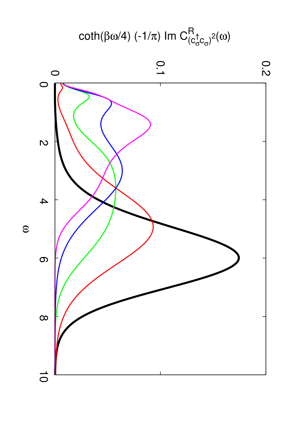
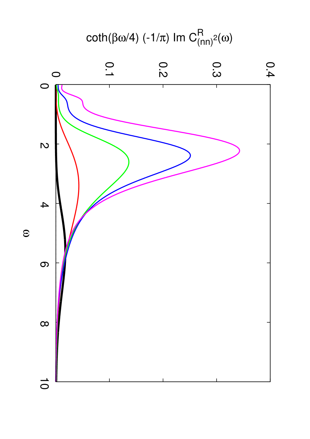
Figure 7 shows the results of the OTOC for the single-orbital Hubbard model. At half filling, this correlation function approaches in the long-time limit and at sufficiently low temperature, so that we perform the analytical continuation procedure for . The top panels of Fig. 7 show the real and imaginary parts of this shifted OTOC. Here, we only present results for the metallic phase, because resolving the very sharp low-energy feature of the OTOC spectrum in the half-filled Mott state is challenging. One can see that coherent oscillations are not observed for this type of OTOC, and that the incoherent part becomes dominant compared to the other two OTOCs shown in Figs. 5 and 6. The amplitude of the OTOC is enhanced as increases. As we argue below, this is related to the enhancement of spin fluctuations and local moment formation close to the Mott transition.
The bottom left panel in Fig. 7 plots the analytically continued spectral function multiplied by . We can see that the spectral weight is concentrated in the low-energy region as we approach the Mott transition point. The inset in the bottom left panel of Fig. 7 shows the imaginary-time four-point function , with the black line corresponding to a Mott insulating solution (). For , the imaginary-time four-point function does not decay to zero but remains relatively large near . This behavior is reminiscent of the spin-freezing physics seen in the correlated Hund metal phase of multi-orbital Hubbard models, where the dynamical spin correlation function is trapped at a finite value at long Werner et al. 2008. In fact, the OTOC measures spin correlations (in addition to charge correlations) through . Physically, the trapping of signals the formation of frozen local magnetic moments. In the metal-insulator crossover region, the scattering induced by these magnetic moments results in incoherent metal states. Intuitively, one might expect fast scrambling in the corresponding regions of the phase diagram. Although there is some resemblance with the spin freezing crossover, the self-energy does not exhibit a square-root frequency dependence in the single-orbital case, and a spin-freezing crossover in the sense of Ref. Werner et al. 2008 does not exist.
The bottom right panel of Fig. 7 plots the modulus of the OTOC (normalized at ) on a log-log scale. The dynamics of is quite distinct from that of . As the Mott transition is approached, we observe a slow-down in the decay of the modulus, which indicates the presence of slowly fluctuating local moments. The long-time behavior may be consistent with a power-law, although slow oscillations make it difficult to determine the long-time asymptotic form from the numerics.

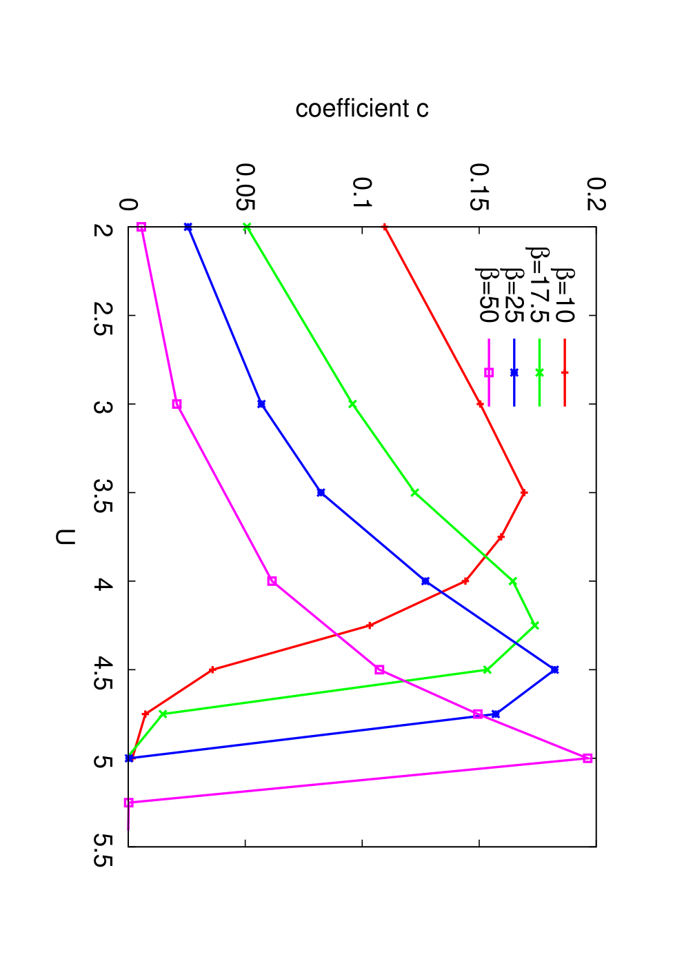
For large enough and small enough , the OTOC (44) factorizes into . On the real-time axis, this corresponds to the decoupling , that is, the OTOC is reduced to a product of ordinary density-density correlation functions. In order to see whether nontrivial correlations are captured beyond the decoupled form by the OTOC function, we consider the difference and fit the short-time behavior of this function to , as illustrated in the left panel of Fig. 8. The coefficients and serve as indicators of the nontrivial correlations that cannot be attributed to the decoupled form of the OTOC. The coefficient is plotted as a function of and for different in the right hand panel. The coefficient (not shown) exhibits a similar trend. We notice that the OTOC picks up nontrival correlations near the metal-insulator transition, and in particular at intermediate temperatures, while the Mott phase shows no such correlations. The crossover region associated with the emergence of local moments corresponds, roughly, to the interaction range where the nontrivial correlations start to become significant.
IV.3 Two-orbital Hubbard model
In this section, we investigate OTOCs in the two-orbital Hubbard model with Hund coupling and density-density interactions. (Three-orbital results are presented in Appendix A.) The Hamiltonian is given by
| (49) |
with being the intra-orbital interaction , the inter-orbital antiparallel-spin interaction, and the inter-orbital parallel-spin interaction. This is the simplest model that shows a crossover from a spin-frozen metal to a Fermi-liquid metal as one dopes the half-filled Mott insulator, with the self-energy scaling as over a significant energy range in the crossover regime Hafermann et al. 2012. The sketch of the phase diagram is shown in Fig. 2. As we have seen in the previous section, the spin-related OTOC of the type (44) is relevant for the analysis of the spin-freezing crossover, so that we concentrate on this OTOC here. In the following calculations, we choose , , and compute as a function of filling at (dashed lines in Fig. 2).
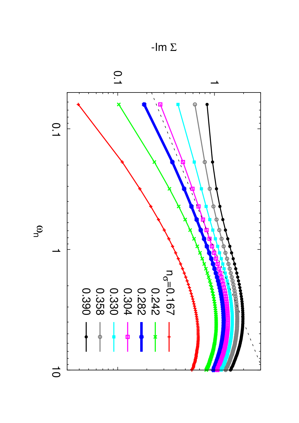

The left panel of Fig. 9 plots the imaginary part of the self-energy as a function of Matsubara frequency in order to identify the filling corresponding to the spin-freezing crossover Werner et al. 2008. An approximate square-root scaling is observed over a wide range of frequencies near (blue line). In the right panel of Fig. 9, we present the coefficient obtained from a similar analysis as presented in Fig. 8, but with a fitting range . Again, we find that the OTOC detects nontrivial correlations in the spin-freezing crossover (blue arrow) and spin-frozen metal regime, but not in the Fermi liquid or the Mott insulating phase.


The top panels of Fig. 10 show the real and imaginary parts of the OTOC for the two-orbital Hubbard model. In the spin-frozen phase (), both components exhibit highly incoherent oscillations, which get suppressed as the filling is reduced. As one moves across the crossover point (), the oscillations completely disappear, and the real part of the OTOC starts to overshoot to the negative side in the Fermi liquid regime. The bottom left panel in Fig. 10 presents the analytically continued spectral function multiplied by . In the spin-frozen regime () a sharp peak appears at low energy, which originates from the saturation of the imaginary-time four point function at large (see the inset of the bottom left panel of Fig. 10). This low-energy peak represents the slow dynamics of the frozen spins, and translates into a slow long-time decay of , as shown in the bottom right panel of Fig. 10 on a log-log scale. Again, it is difficult to clearly resolve the long-time behavior of the OTOC due to the limited accuracy of the analytic continuation, but in the spin-freezing crossover regime (thick blue curves) the decay of the OTOC is consistent with a power law at least for . The shorter-time behavior () is instead well fitted by an exponential decay with a decay constant . This exponent exhibits a strong dependence on the Hund coupling. In fact, the OTOCs in the spin-freezing regime for and can be approximately collapsed by plotting them as a function of (see the inset in the bottom right panel of Fig. 10), which indicates that the Hund coupling is the parameter which controls the dynamics in this regime. This is distinct from the Lyapunov behavior in which the exponential decay scales with Bagrets et al. 2017. A possible reason is that we are still far from the large limit (where corresponds to the number of orbitals times the number of spin degrees of freedom) so that the large behavior such as the Lyapunov growth is not observed in our calculations. In fact, the strong dependence of the time scale on and weak dependence on is consistent with the behavior of the finite SYK model in Ref. Fu and Sachdev 2016. In the spin-frozen regime () the decay is much slower than near the crossover point, while in the Fermi liquid regime the decay is accelerated, approaching the free fermion behavior of as shown in Fig. 3. Qualitatively similar results for this OTOC are obtained for the three-orbital Hubbard model (see Appendix A).
The time dependence of the modulus of in the spin-freezing crossover regime of multi-orbital Hubbard models (exponential decay crossing over into a power-law) bears a close resemblance to a (different) OTOC for the SYK model discussed in Ref. Bagrets et al. 2017. Also, a recent study of yet another type of OTOCs for the finite- SYK model found a qualitatively similar decay as observed here in the spin-freezing crossover regime Fu and Sachdev 2016. In the following section, we will make the connection to the SYK dynamics more quantitative.
IV.4 Comparison to the SKY model
In this section, we compare the results of the multi-orbital Hubbard models to the SYK model. We consider the particle-hole symmetric SYK model of complex fermions Fu and Sachdev 2016, whose Hamiltonian is given by
| (50) |
The coupling constant is a gaussian random variable, satisfying , and
| (51) | ||||
| (52) |
where the overline represents an average over each realization of . The parameter () defines the unit of energy (time) in the following calculations. The system is particle-hole symmetric when , which fixes the total number of fermions as . We take the particle-hole symmetric form of the SYK model because it has been well studied previously Fu and Sachdev 2016 and avoids the effect of the filling drift. We numerically solve the model by exact diagonalization for finite , and evaluate the density-density OTOC and its imaginary-time counterpart.


In the left panel of Fig. 11, we plot the imaginary-time four-point function for the SYK model with and . At low temperature, we expect that is decoupled into . To see whether nontrivial correlations beyond the decoupled form are present, we fit the difference with a function in the interval , in the same manner as for the Hubbard models. The obtained coefficient is plotted as a function of the temperature in the right panel of Fig. 11. One can see that nontrivial correlations exist in a wide range of temperature. Especially, they are enhanced in the intermediate temperature regime. This is because in the zero-temperature limit the four-point function is decoupled as , while in the high-temperature limit () the imaginary-time dependence is washed out.


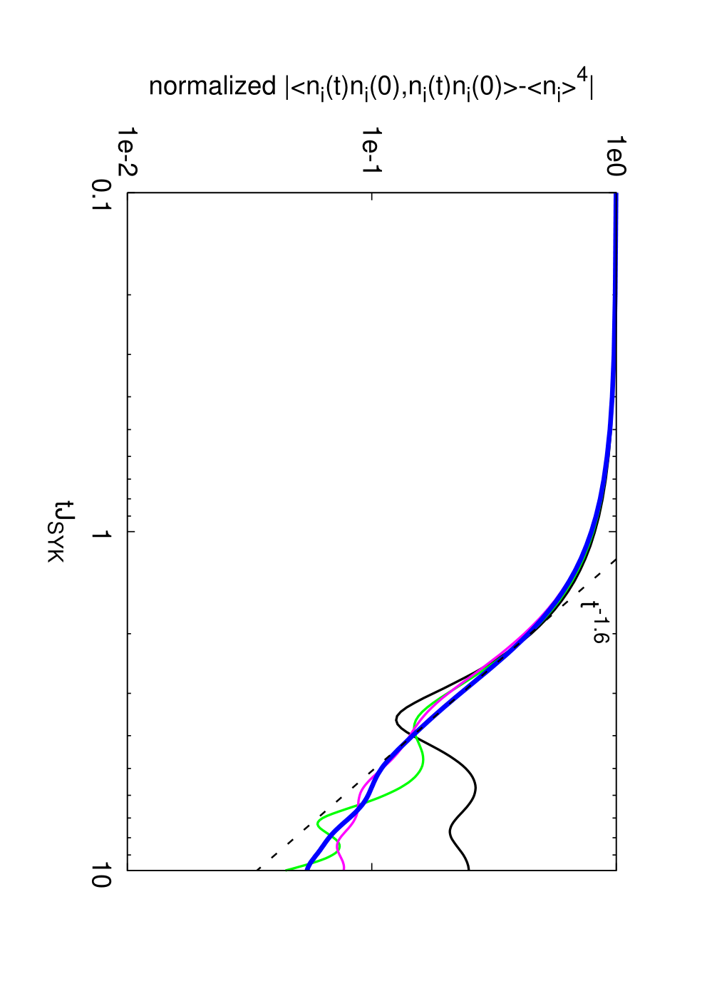
In Fig. 12, we show the numerical results of the density-density OTOC for . The real part of the OTOC rapidly drops from the initial value within the time scale of , and slowly decays to zero in the long time limit. As one increases , the oscillations that appear at longer time tend to be suppressed. One can see that the result for in the top panels of Fig. 12 closely resembles the OTOC in the spin-freezing crossover regime of the two-orbital Hubbard model shown by the blue curve in the top panels of Fig. 10, while it differs from the single-orbital result shown in the top panels of Fig. 7. Due to the limitation of our calculations to small system sizes (), we do not clearly observe an exponential growth () at short times or an exponential decay () at intermediate times. However, we find that for the OTOC decays approximately in a power law with (see bottom right panel in Fig. 12). The time interval exhibiting the power-law decay becomes longer as we increase . The temperature dependence of the OTOC for the SYK model is shown in Fig. 13. The time scale of the initial drop is more or less independent of the temperature, while the power-law-like decay is only visible in the low-temperature regime.


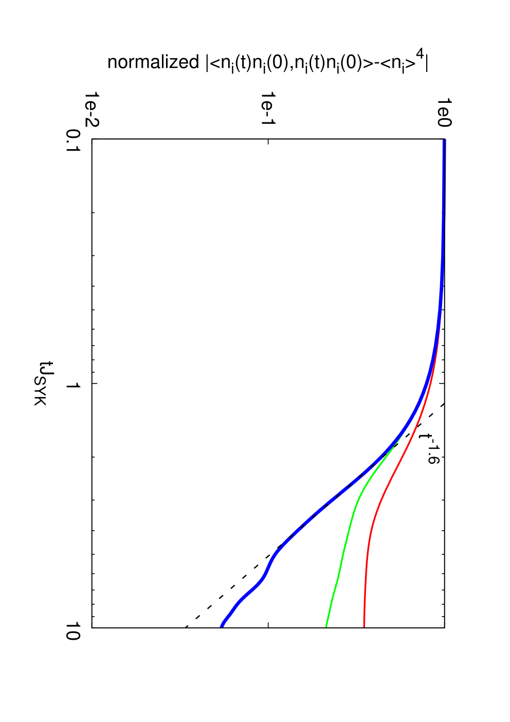
In Ref. Wer, it has been argued that the spin-freezing crossover regime of multi-orbital Hubbard models is effectively described by the SYK model in which is replaced by the Hund coupling . The results in Fig. 10 are for the two-orbital Hubbard model with , and , corresponding to , which means that it is meaningful to directly compare the blue lines in Fig. 10 with the blue lines in Figs. 12 and 13. Not only is the qualitative agreement remarkable, even the power-law exponent measured for the two-orbital Hubbard model () is very close to the exponent extracted from the finite- SYK calculation. The power-law decay in the three-orbital case is approximately (see Appendix A), and thus also in semi-quantitative agreement with the SYK model behavior. This nontrivial result provides further support for the identification of the spin-freezing crossover regime of multi-orbital Hubbard systems with an SYK strange metal.
In the large- and low- limit of the SYK model, we expect that the power-law behavior approaches , since in this limit the OTOC is decoupled as and the decay of is dominated by what corresponds to the slow spin relaxation in the Sachdev-Ye model.
V Conclusions
We have studied out-of-time-ordered correlators for single- and multi-orbital Hubbard models on the infinitely connected Bethe lattice using DMFT simulations combined with an analytical continuation procedure. The basis for this approach is the fact that real-time OTOCs and suitably defined imaginary-time four-point correlation functions are analytically connected through the spectral representation and the out-of-time-order fluctuation-dissipation theorem. We showed that it allows to accurately compute the short-time dynamics of OTOCs (up to a few inverse hopping times), as well as the rough decay at long times, which is controlled by low-energy spectral features. The details of oscillations at intermediate and long times can, however, not be accurately captured by the analytical continuation method.
We have used this novel procedure to explore OTOCs in the correlated metal phase, with a particular focus on the spin-related OTOC which detects the formation of local moments. In the context of the recently proposed connection between the spin-freezing crossover regime of multi-orbital Hubbard models and the SYK model, it is particularly interesting to investigate the doped Mott regime of multi-orbital systems with nonzero Hund coupling. We found that the spin-freezing crossover regime, which is characterized by a behavior of the self-energy and a decay of the spin correlations, is reflected in a qualitative change of the short-time decay of the spin-related OTOC. More specifically, the real part of this OTOC changes from a slowly decaying function in the weakly doped bad metal phase with frozen magnetic moments to a fast decaying and overshooting function in the strongly doped Fermi liquid phase. In the spin-freezing crossover region, the modulus of the OTOC exhibits an approximately exponential short-time decay, which crosses over into a power-law at , and the results for different can be approximately collapsed by plotting the OTOC as a function of . The power-law exponents are similar for the two- and three-orbital models ( and 1.75, respectively), and in almost quantitative agreement with the result for the finite- SYK model ().
Our results provide further evidence that the spin-freezing crossover regime of multi-orbital Hubbard models is effectively described by the SYK model, and that in this context can be identified with the Hund coupling parameter, which differentiates between the energies of same-spin and opposite spin inter-orbital interactions. The SYK model is thus relevant for the description of an important class of correlated materials, the so-called Hund metals Georges et al. 2013, which includes a broad range of unconventional superconductors, such as Sr2RuO4 and iron-based superconductors. Via a suitable mapping, it also becomes relevant for the description of optimally doped cuprates Werner et al. 2016.
In a broader context, our work demonstrates a general strategy for calculating real-time OTOCs of interacting lattice models in the thermodynamic limit. This opens the door to systematic explorations of strange metal physics and information scrambling based on OTOCs in models that are relevant for the description of condensed matter systems.
Acknowledgements.
The DMFT calculations were performed on the Beo04 cluster at the University of Fribourg, using a code based on ALPS Albuquerque et al. 2007. N.T. is supported by JSPS KAKENHI Grant No. JP16K17729. P.W. thanks the Aspen Center for Physics for its hospitality. Most of the numerical work was carried out during the 2017 summer workshop on “Correlations and Entanglement in and out of Equilibrium: from Cold Atoms to Electrons” and the 2018 workshop on “Topological Phases and Excitations of Quantum Matter.”Appendix A Results for the three-orbital Hubbard model


We show the results for the self-energy and the modulus of the OTOC for the three-orbital Hubbard model with , , and in Fig. 14. The spin-freezing crossover roughly occurs at the filling (blue lines), where we observe an approximate power-law decay of the modulus of the OTOC (44) at longer times, with .
References
- Sachdev and Ye (1993) S. Sachdev and J. Ye, “Gapless Spin-Fluid Ground State in a Random Quantum Heisenberg Magnet,” Phys. Rev. Lett. 70, 3339 (1993).
- Georges et al. (2000) A. Georges, O. Parcollet, and S. Sachdev, “Mean Field Theory of a Quantum Heisenberg Spin Glass,” Phys. Rev. Lett. 85, 840 (2000).
- Georges et al. (2001) A. Georges, O. Parcollet, and S. Sachdev, “Quantum fluctuations of a nearly critical Heisenberg spin glass,” Phys. Rev. B 63, 134406 (2001).
- Parcollet et al. (1998) O. Parcollet, A. Georges, G. Kotliar, and A. Sengupta, “Overscreened multichannel Kondo model: Large- solution and conformal field theory,” Phys. Rev. B 58, 3794 (1998).
- Parcollet and Georges (1999) O. Parcollet and A. Georges, “Non-Fermi-liquid regime of a doped Mott insulator,” Phys. Rev. B 59, 5341 (1999).
- (6) A. Kitaev, “A simple model of holography”, KITP Program: Entanglement in Strongly-Correlated Quantum Matter (2015): http://online.kitp.ucsb.edu/online/entangled15/kitaev/, http://online.kitp.ucsb.edu/online/entangled15/kitaev2/.
- Sachdev (2015) S. Sachdev, “Bekenstein-Hawking Entropy and Strange Metals,” Phys. Rev. X 5, 041025 (2015).
- Polchinski and Rosenhaus (2016) J. Polchinski and V. Rosenhaus, “The spectrum in the Sachdev-Ye-Kitaev model,” J. High Energy Phys. 04, 001 (2016).
- Maldacena and Stanford (2016) J. Maldacena and D. Stanford, “Remarks on the Sachdev-Ye-Kitaev model,” Phys. Rev. D 94, 106002 (2016).
- Larkin and Ovchinnikov (1969) A. I. Larkin and Y. N. Ovchinnikov, “Quasiclassical method in the theory of superconductivity,” Sov. Phys. JETP 28, 1200 (1969).
- Shenker and Stanford (2014a) S. H. Shenker and D. Stanford, “Black holes and the butterfly effect,” J. High Energy Phys. 03, 067 (2014a).
- Shenker and Stanford (2014b) S. H. Shenker and D. Stanford, “Multiple shocks,” J. High Energy Phys. 12, 046 (2014b).
- Shenker and Stanford (2015) S. H. Shenker and D. Stanford, “Stringy effects in scrambling,” J. High Energy Phys. 05, 132 (2015).
- Maldacena et al. (2016) J. Maldacena, S. H. Shenker, and D. Stanford, “A bound on chaos,” J. High Energy Phys. 08, 106 (2016).
- Hosur et al. (2016) P. Hosur, X.-L. Qi, D. A. Roberts, and B. Yoshida, “Chaos in quantum channels,” J. High Energy Phys. 02, 004 (2016).
- Swingle et al. (2016) B. Swingle, G. Bentsen, M. Schleier-Smith, and P. Hayden, “Measuring the scrambling of quantum information,” Phys. Rev. A 94, 040302(R) (2016).
- Gärttner et al. (2017) M. Gärttner, J. G. Bohnet, A. Safavi-Naini, M. L. Wall, J. J. Bollinger, and A. M. Rey, “Measuring Out-of-time-order Correlations and Multiple Quantum Spectra in a Trapped-ion Quantum Magnet,” Nat. Phys. 13, 781 (2017).
- Li et al. (2017) J. Li, R. Fan, H. Wang, B. Ye, B. Zeng, H. Zhai, X. Peng, and J. Du, “Measuring Out-of-Time-Order Correlators on a Nuclear Magnetic Resonance Quantum Simulator,” Phys. Rev. X 7, 031011 (2017).
- (19) E. J. Meier, J. Ang’ong’a, F. A. An, and B. Gadway, arXiv:1705.06714.
- Tsuji et al. (2018a) N. Tsuji, T. Shitara, and M. Ueda, “Bound on the exponential growth rate of out-of-time-ordered correlators,” Phys. Rev. E 98, 012216 (2018a).
- Bagrets et al. (2017) D. Bagrets, A. Altland, and A. Kamenev, “Power-law out of time order correlation functions in the SYK model,” Nucl. Phys. B 921, 727 – 752 (2017).
- Gu et al. (2017) Y. Gu, X.-L. Qi, and D. Stanford, “Local criticality, diffusion and chaos in generalized Sachdev-Ye-Kitaev models,” J. High Energy Phys. 05, 125 (2017).
- Davison et al. (2017) R. A. Davison, W. Fu, A. Georges, Y. Gu, K. Jensen, and S. Sachdev, “Thermoelectric transport in disordered metals without quasiparticles: The Sachdev-Ye-Kitaev models and holography,” Phys. Rev. B 95, 155131 (2017).
- Song et al. (2017) X.-Y. Song, C.-M. Jian, and L. Balents, “Strongly Correlated Metal Built from Sachdev-Ye-Kitaev Models,” Phys. Rev. Lett. 119, 216601 (2017).
- Chowdhury et al. (2018) D. Chowdhury, Y. Werman, E. Berg, and T. Senthil, “Translationally Invariant Non-Fermi-Liquid Metals with Critical Fermi Surfaces: Solvable Models,” Phys. Rev. X 8, 031024 (2018).
- Danshita et al. (2017) I. Danshita, M. Hanada, and M. Tezuka, “Creating and probing the Sachdev-Ye-Kitaev model with ultracold gases: Towards experimental studies of quantum gravity,” Prog. Theor. Exp. Phys. 2017, 083I01 (2017).
- García-Álvarez et al. (2017) L. García-Álvarez, I. L. Egusquiza, L. Lamata, A. del Campo, J. Sonner, and E. Solano, “Digital Quantum Simulation of Minimal ,” Phys. Rev. Lett. 119, 040501 (2017).
- Pikulin and Franz (2017) D. I. Pikulin and M. Franz, “Black Hole on a Chip: Proposal for a Physical Realization of the Sachdev-Ye-Kitaev model in a Solid-State System,” Phys. Rev. X 7, 031006 (2017).
- Chen et al. (2018) A. Chen, R. Ilan, F. de Juan, D. I. Pikulin, and M. Franz, “Quantum Holography in a Graphene Flake with an Irregular Boundary,” Phys. Rev. Lett. 121, 036403 (2018).
- (30) P. Werner, A. Kim, and S. Hoshino, “Spin freezing and the Sachdev-Ye model”, arXiv:1805.04102.
- Werner et al. (2008) P. Werner, E. Gull, M. Troyer, and A. J. Millis, “Spin Freezing Transition and Non-Fermi-Liquid Self-Energy in a Three-Orbital model,” Phys. Rev. Lett. 101, 166405 (2008).
- Ishida and Liebsch (2010) H. Ishida and A. Liebsch, “Fermi-liquid, non-Fermi-liquid, and Mott phases in iron pnictides and cuprates,” Phys. Rev. B 81, 054513 (2010).
- de’ Medici et al. (2011) L. de’ Medici, J. Mravlje, and A. Georges, “Janus-Faced Influence of Hund’s Rule Coupling in Strongly Correlated Materials,” Phys. Rev. Lett. 107, 256401 (2011).
- Hoshino and Werner (2015) S. Hoshino and P. Werner, “Superconductivity from Emerging Magnetic Moments,” Phys. Rev. Lett. 115, 247001 (2015).
- Stadler et al. (2015) K. M. Stadler, Z. P. Yin, J. von Delft, G. Kotliar, and A. Weichselbaum, “Dynamical Mean-Field Theory Plus Numerical Renormalization-Group Study of Spin-Orbital Separation in a Three-Band Hund Metal,” Phys. Rev. Lett. 115, 136401 (2015).
- García-García et al. (2018) A. M. García-García, B. Loureiro, A. Romero-Bermúdez, and M. Tezuka, “Chaotic-Integrable Transition in the Sachdev-Ye-Kitaev Model,” Phys. Rev. Lett. 120, 241603 (2018).
- Banerjee and Altman (2017) S. Banerjee and E. Altman, “Solvable model for a dynamical quantum phase transition from fast to slow scrambling,” Phys. Rev. B 95, 134302 (2017).
- Rozenbaum et al. (2017) E. B. Rozenbaum, S. Ganeshan, and V. Galitski, “Lyapunov Exponent and Out-of-Time-Ordered Correlator’s Growth Rate in a Chaotic System,” Phys. Rev. Lett. 118, 086801 (2017).
- (39) E. B. Rozenbaum, S. Ganeshan, and V. Galitski, “Universal Level Statistics of the Out-of-Time-Ordered Operator”, arXiv:1801.10591.
- Aleiner et al. (2016) I. L. Aleiner, L. Faoro, and L. B. Ioffe, “Microscopic model of quantum butterfly effect: Out-of-time-order correlators and traveling combustion waves,” Ann. Phys. 375, 378 (2016).
- Stanford (2016) D. Stanford, “Many-body chaos at weak coupling,” J. High Energy Phys. 10, 009 (2016).
- Patel and Sachdev (2017) A. A. Patel and S. Sachdev, “Quantum chaos on a critical fermi surface,” Proc. Natl. Acad. Sci. U.S.A. 114, 1844 (2017).
- Patel et al. (2017) A. A. Patel, D. Chowdhury, S. Sachdev, and B. Swingle, “Quantum butterfly effect in weakly interacting diffusive metals,” Phys. Rev. X 7, 031047 (2017).
- Chowdhury and Swingle (2017) D. Chowdhury and B. Swingle, “Onset of many-body chaos in the model,” Phys. Rev. D 96, 065005 (2017).
- Liao and Galitski (2018) Y. Liao and V. Galitski, “Nonlinear sigma model approach to many-body quantum chaos: Regularized and unregularized out-of-time-ordered correlators,” Phys. Rev. B 98, 205124 (2018).
- (46) X. Chen, T. Zhou, D. A. Huse, and E. Fradkin, “Out-of-time-order correlations in many-body localized and thermal phases”, Ann. Phys. 529, 1600332 (2016).
- Fan et al. (2017) R. Fan, P. Zhang, H. Shen, and H. Zhai, “Out-of-time-order correlation for many-body localization,” Sci. Bull. 62, 707 (2017).
- Fu and Sachdev (2016) W. Fu and S. Sachdev, “Numerical study of fermion and boson models with infinite-range random interactions,” Phys. Rev. B 94, 035135 (2016).
- He and Lu (2017) R.-Q. He and Z.-Y. Lu, “Characterizing many-body localization by out-of-time-ordered correlation,” Phys. Rev. B 95, 054201 (2017).
- Huang et al. (2016) Y. Huang, Y.-L. Zhang, and X. Chen, “Out-of-time-ordered correlators in many-body localized systems,” Ann. Phys. 529, 1600318 (2016).
- Shen et al. (2017) H. Shen, P. Zhang, R. Fan, and H. Zhai, “Out-of-time-order correlation at a quantum phase transition,” Phys. Rev. B 96, 054503 (2017).
- (52) N. Y. Yao, F. Grusdt, B. Swingle, M. D. Lukin, D. M. Stamper-Kurn, J. E. Moore, and E. Demler, “Interferometric Approach to Probing Fast Scrambling”, arXiv:1607.01801.
- Bohrdt et al. (2017) A. Bohrdt, C. B. Mendl, M. Endres, and M. Knap, “Scrambling and thermalization in a diffusive quantum many-body system,” New J. Phys. 19, 063001 (2017).
- Dóra and Moessner (2017) B. Dóra and R. Moessner, “Out-of-Time-Ordered Density Correlators in Luttinger Liquids,” Phys. Rev. Lett. 119, 026802 (2017).
- Dóra et al. (2017) B. Dóra, M. A. Werner, and C. P. Moca, “Information scrambling at an impurity quantum critical point,” Phys. Rev. B 96, 155116 (2017).
- Georges et al. (1996) A. Georges, G. Kotliar, W. Krauth, and M. J. Rozenberg, “Dynamical mean-field theory of strongly correlated fermion systems and the limit of infinite dimensions,” Rev. Mod. Phys. 68, 13 (1996).
- Metzner and Vollhardt (1989) W. Metzner and D. Vollhardt, “Correlated Lattice Fermions in Dimensions,” Phys. Rev. Lett. 62, 324 (1989).
- Aoki et al. (2014) H. Aoki, N. Tsuji, M. Eckstein, M. Kollar, T. Oka, and P. Werner, “Nonequilibrium dynamical mean-field theory and its applications,” Rev. Mod. Phys. 86, 779 (2014).
- Tsuji et al. (2017) N. Tsuji, P. Werner, and M. Ueda, “Exact out-of-time-ordered correlation functions for an interacting lattice fermion model,” Phys. Rev. A 95, 011601(R) (2017).
- Freericks and Zlatić (2003) J. K. Freericks and V. Zlatić, “Exact dynamical mean-field theory of the Falicov-Kimball model,” Rev. Mod. Phys. 75, 1333 (2003).
- Tsuji et al. (2018b) N. Tsuji, T. Shitara, and M. Ueda, “Out-of-time-order fluctuation-dissipation theorem,” Phys. Rev. E 97, 012101 (2018b).
- Gull et al. (2011) E. Gull, A. J. Millis, A. I. Lichtenstein, A. N. Rubtsov, M. Troyer, and P. Werner, “Continuous-time Monte Carlo methods for quantum impurity models,” Rev. Mod. Phys. 83, 349 (2011).
- Werner et al. (2009) P. Werner, T. Oka, and A. J. Millis, “Diagrammatic Monte Carlo simulation of nonequilibrium systems,” Phys. Rev. B 79, 035320 (2009).
- Wigner and Yanase (1963) E. P. Wigner and M. M. Yanase, “Information contents of distributions,” Proc. Natl. Acad. Sci. U.S.A. 49, 910 (1963).
- Luo (2005) S. L. Luo, “Quantum versus classical uncertainty,” Theor. Math. Phys. 143, 681 (2005).
- Werner et al. (2006) P. Werner, A. Comanac, L. de’ Medici, M. Troyer, and A. J. Millis, “Continuous-Time Solver for Quantum Impurity Models,” Phys. Rev. Lett. 97, 076405 (2006).
- Werner and Millis (2006) P. Werner and A. J. Millis, “Hybridization expansion impurity solver: General formulation and application to Kondo lattice and two-orbital models,” Phys. Rev. B 74, 155107 (2006).
- Jarrell and Gubernatis (1996) M. Jarrell and J. E. Gubernatis, “Bayesian inference and the analytic continuation of imaginary-time quantum Monte Carlo data,” Phys. Rep. 269, 133 (1996).
- (69) https://bitbucket.org/lewinboehnke/maxent.
- (70) N. Blümer, PhD Thesis, Universität Augsburg, (2002).
- Hafermann et al. (2012) H. Hafermann, K. R. Patton, and P. Werner, “Improved estimators for the self-energy and vertex function in hybridization-expansion continuous-time quantum Monte Carlo simulations,” Phys. Rev. B 85, 205106 (2012).
- Georges et al. (2013) A. Georges, L. de’ Medici, and J. Mravlje, “Strong Correlations from Hund’s Coupling,” Ann. Rev. Condens. Matter Phys. 4, 137 (2013).
- Werner et al. (2016) P. Werner, S. Hoshino, and H. Shinaoka, “Spin-freezing perspective on cuprates,” Phys. Rev. B 94, 245134 (2016).
- Albuquerque et al. (2007) A. F. Albuquerque, F. Alet, P. Corboz, P. Dayal, A. Feiguin, S. Fuchs, L. Gamper, E. Gull, S. Guertler, A. Honecker, R. Igarashi, M. Koerner, A. Kozhevnikov, A. Laeuchli, S. R. Manmana, M. Matsumoto, I. P. McCulloch, F. Michel, R. M. Noack, G. Pawowski, L. Pollet, T. Pruschke, U. Schollwoeck, S. Todo, S. Trebst, M. Troyer, P. Werner, and S. Wessel, “The ALPS project release 1.3: Open-source software for strongly correlated systems,” J. Magn. Magn. Mater. 310, 1187 (2007).