跳到论文正文
W Papers独立论文阅读器 arXiv:1812.04212 论文正文 计算阅读时间 · 0%
引用这篇论文根据当前论文元数据生成,正式投稿前建议核对。


License: arXiv.org perpetual non-exclusive license
arXiv:1812.04212v1 [nlin.SI] 11 Dec 2018

Multi-breathers and high order rogue waves for the nonlinear Schrödinger equation on the elliptic function background

Bao-Feng Feng Address: School of Mathematical and Statistical Sciences, The University of Texas Rio Grande Valley Edinburg TX, 78541-2999, USA Email address: baofeng.feng@utrgv.edu , Liming Ling Address: School of Mathematics, South China University of Technology, Guangzhou, 510641, China Email address: linglm@scut.edu.cn; lingliming@qq.com and Daisuke A. Takahashi Address: Research and Education Center for Natural Sciences, Keio University, Hiyoshi 4-1-1, Yokohama, Kanagawa 223-8521, Japan Email address: daisuke.takahashi@keio.jp
Date: August 11, 2026
Abstract.

We construct the multi-breather solutions of the focusing nonlinear Schrödinger equation (NLSE) on the background of elliptic functions by the Darboux transformation, and express them in terms of the determinant of theta functions. The dynamics of the breathers in the presence of various kinds of backgrounds such as dn, cn, and non-trivial phase-modulating elliptic solutions are presented, and their behaviors dependent on the effect of backgrounds are elucidated. We also determine the asymptotic behaviors for the multi-breather solutions with different velocities in the limit t→±∞t\to\pm\infty, where the solution in the neighborhood of each breather tends to the simple one-breather solution. Furthermore, we exactly solve the linearized NLSE using the squared eigenfunction and determine the unstable spectra for elliptic function background. By using them, the Akhmediev breathers arising from these modulational instabilities are plotted and their dynamics are revealed. Finally, we provide the rogue-wave and higher-order rogue-wave solutions by taking the special limit of the breather solutions at branch points and the generalized Darboux transformation. The resulting dynamics of the rogue waves involves rich phenomena: depending on the choice of the background and possessing different velocities relative to the background. We also provide an example of the multi- and higher-order rogue wave solution.

1. Introduction

As a universal model in the description of the propagation of a quasi-monochromatic wave in a weakly nonlinear medium, the nonlinear Schrödinger equation (NLSE) has played a central role in mathematical physics and integrable partial differential equations [18]. It is relevant in numerous applications of natural sciences such as water waves, nonlinear optics, plasmas, Bose-Einstein condensates. For the zero background, a variety of methods either for the analysis of the Cauchy problem or the systematic construction of the multi-soliton solutions has been well established for a long time. A nonzero with plane wave background can be unstable under the perturbation, and this modulation instability (MI) is considered as the main cause for the formation of rogue waves (RWs) in nature. The integrable nature of the NLSE allows one to construct a family of exact solutions corresponding to this nonzero plane wave background by different methods such as the generalized Darboux transformation method, the dressing method, the inverse scattering method and Hirota bilinear method. Since the 70s, there are lots of works on the integrable NLSE model; giving a complete account of the reference on the relative subject is out of the scope of this introduction.

Recent study by Grinevich and Santini [19] (equations (48)-(49) ) shows finite-gap soliton solutions of genius-1 or genius-2 may be developed from a Cauchy problem of the NLSE with a very small perturbation. For the genius-1 case, a nonzero background expressed by elliptic function is formed before the rogue wave solution or the Akhmediev breather solution is formed. In this sense, the rogue wave or Akhmediev breather solutions with complicated backgrounds such as elliptic functions are more natural and are expected to occur in experiments. Actually, Akhmediev et al. have studied this kind of solution in a simple setting [24]. Due to the mathematical difficulty, the study of constructing soliton solutions with elliptic function background is much less and nontrivial. In this paper, one aim is to construct general breathers and rogue waves of the NLSE with the elliptic function background systematically.

From the theoretical point of view, the systematic construction of the multi-soliton solutions on the elliptic function background can be broadly classified into two categories. The first method is to take the limit in the higher-genus solutions constructed by the algebro-geometric method [3] or the Riemann-Hilbert method. The other way is using the inverse scattering method or the Darboux transformation [7, 9, 15, 20, 21, 30] to construct the breathers by the linear algebra. However, both methods have different difficulties. For the first way, it is hard to analyze the different limitation and deal with lots of elliptic integration, while for the second way, the obtained formula by the linear algebra is easy, but it is difficult to analyze the properties for the determinant.

Firstly, we review several known results on this aspect. In the section 4.5 of monograph [3], the authors considered the degenerate finite-gap solution—multi-phase modulations of the cnoidal wave for the defocusing NLSE by taking the limit and used the complex coordinate transformation x→i​xx\to\mathrm{i}x to derive multi Akhmediev breathers on the dn{\rm dn} function background [3]. Recently, Shin considered the single soliton dynamics in phase-modulated lattices by Darboux transformation by modified squared wavefunction approach [34]. A compact formula for the single breather solution was not, however, given explicitly, and hence the shift of the crest and phase was not analyzed. The exact solitons on the elliptic function background are constructed by the eigenfunction symmetry method [13, 32]. Breathers, rogue waves and higher order rogue waves on the dn and cn background are obtained by numerically solving the Lax pair equation and Darboux transformation [2, 24]. The solitons for the defocusing NLSE on the elliptic function background was obtained by the inverse scattering method [36], where the seed eigenfunction of the Lax pair was obtained using the result of [37], and the solution was expressed by the determinant of theta function. The rogue waves for the focusing NLSE on the cn and dn background are obtained by combining the Darboux transformation with nonlinearization of the Lax pair [12]. Meanwhile, there are some relevant works on the rogue waves on the higher genus solutions [4], in which the analytical criterion to generalized rogue waves are obtained by the Riemann-Hilbert method. The bounded ultra-elliptic solutions for the defocusing NLSE are considered by the effective integration method [38]. The various initial data for the semiclassical NLSE are related with the rogue-wave phenomena [33, 5, 17].

Even though there are some contributions on this subject, there is not systematic theory to construct the breathers and rogue waves on the elliptic function background. What is more important is that there is no method to analyze the solutions generated by the Darboux transformation. In this work, we would like to address these issues. The key step to generate the solution by the Darboux transformation is solving the Lax pair equation with the seed solution. Once it can be obtained, plugging the vector solutions of the Lax pair into the Bäcklund transformation induced by the Darboux transformation, we get the new solutions. Since the formula of the Bäcklund transformation is algebraic, the new solutions are obtained exactly, and furthermore, this operation can be iterated as many times as desired. Therefore, the family of the multi-fold and higher-order solutions can be obtained recursively. The closed-form multi-breather solutions can be easily plotted by just setting the parameters, and no numerical computation is necessary.

However, since the solutions generated by the Darboux transformation involve lots of free non-trivial parameters, if we want to understand their effect precisely, the formulas found from the Bäcklund transformation are not always useful for observation of the general laws of the dynamics. Thus we need to reduce the formula in a proper form, so that the dynamics of solutions can be analyzed. In this work, we use the addition formulas of theta functions to rewrite the expressions of the multi-soliton solutions. In this way, the general dynamics can be analyzed directly through the asymptotic analysis of the determinant formula.

It is well known that the breather solutions in the focusing NLSE involve the special and important limiting cases, which have a close relation to the modulational instability. The elliptic-function solutions for the focusing NLSE are also known to be unstable [16]. It is therefore natural to construct the exact solutions to describe the unstable process. Thus, the second aim in this work is to construct the Akhmediev breathers on the elliptic function background, which is helpful to understand the mechanism of modulational instability.

Finally, for the rogue waves, it is also related with the modulational instability with infinite period. The comprehensive construction for higher order rogue waves with the closed expressions has been open so far. In this work, we prove that the formulas of higher order rogue waves can be represented as a rational functions of xx, tt, the Jacobi elliptic functions sn{\rm sn}, cn{\rm cn}, dn{\rm dn} and the second type of elliptic integral.

The rest of this paper is organized as the follows. In section 2 we solve the Lax pair with the elliptic function by combining the algebro-geometric method and the modified squared wavefunction approach. As a byproduct of the modified squared wavefunction approach, we also solve the linearized NLSE directly, which is useful for the analysis of the modulational instability. In section 3, we construct the breathers and multi-breathers on the elliptic function background. Furthermore, with the aid of the addition formula for the theta function, we rewrite them in a determinant form. Their dynamics are also investigated for various backgrounds. In section 4, we determine the unstable spectra for the linearized NLSE, and analyze the corresponding Akhmediev breathers on the elliptic-function background, which is related with the modulational instability. In section 5, we provide the rogue waves and high order rogue waves. We further discuss the effect of the choice of backgrounds to the dynamics of rogue waves. Section 6 is devoted to the conclusion and discussion.

2. The elliptic function solution of NLSE and its Lax pair

In this section, we derive the elliptic function solution for NLSE firstly and then the corresponding solutions for the Lax pair are solved with the aid of algebraic geometry method. The scheme is given in details in the monograph [3]. Here we just focus on the genus one case, in which we can use the elliptic functions and integrals to represent these solutions instead of the Abel map and Riemann theta function. In the following, we give the details to construct the solutions.

The NLSE reads

(2.1) i​ψt+12​ψx​x+|ψ|2​ψ=0,{\rm i}\psi_{t}+\frac{1}{2}\psi_{xx}+|\psi|^{2}\psi=0,

which admits the following Lax pair:

(2.2) Φx=𝐔(𝐐;λ)Φ,𝐔(𝐐;λ)=−iλσ3+i𝐐,Φt=𝐕(𝐐;λ)Φ,𝐕(𝐐;λ)=−iλ2σ3+λi𝐐+𝐕0,𝐕0=12σ3(i𝐐2−𝐐x),\begin{split}{\Phi}_{x}&=\mathbf{U}(\mathbf{Q};\lambda){\Phi},\,\,\mathbf{U}(\mathbf{Q};\lambda)=-{\rm i}\lambda\sigma_{3}+{\rm i}\mathbf{Q},\\ {\Phi}_{t}&=\mathbf{V}(\mathbf{Q};\lambda){\Phi},\,\,\mathbf{V}(\mathbf{Q};\lambda)=-{\rm i}\lambda^{2}\sigma_{3}+\lambda{\rm i}\mathbf{Q}+\mathbf{V}_{0},\,\,\,\,\mathbf{V}_{0}=\frac{1}{2}\sigma_{3}({\rm i}\mathbf{Q}^{2}-\mathbf{Q}_{x}),\end{split}

where

σ3=[100−1],𝐐=[0ψψ∗0].\sigma_{3}=\begin{bmatrix}1&0\\ 0&-1\end{bmatrix},\,\,\,\,\,\,\mathbf{Q}=\begin{bmatrix}0&\psi\\ \psi^{*}&0\end{bmatrix}.

In other words, the compatibility condition Φx​t=Φt​x\Phi_{xt}=\Phi_{tx} or the zero curvature condition 𝐔t−𝐕x+[𝐔,𝐕]=0\mathbf{U}_{t}-\mathbf{V}_{x}+[\mathbf{U},\mathbf{V}]=0 yields the NLSE (2.1). It is readily to see the symmetry for the potential function 𝐔\mathbf{U} and 𝐕\mathbf{V}: 𝐔†​(𝐐,λ∗)=−𝐔⁡(𝐐,λ)\mathbf{U}^{{\dagger}}(\mathbf{Q};\lambda^{*})=-\mathbf{U}(\mathbf{Q};\lambda) and 𝐕†​(𝐐,λ∗)=−𝐕⁡(𝐐,λ)\mathbf{V}^{{\dagger}}(\mathbf{Q};\lambda^{*})=-\mathbf{V}(\mathbf{Q};\lambda), where † denotes the hermitian conjugate. Based on the above symmetry, if Φ⁡(x,t,λ)\Phi(x,t;\lambda) is a matrix solution for Lax pair (2.2), then Φ†​(x,t,λ∗)\Phi^{{\dagger}}(x,t;\lambda^{*}) is a matrix solution for the adjoint Lax pair of (2.2). As a general symmetry, if Φ⁡(x,t,λ)\Phi(x,t;\lambda) satisfies the Lax pair (2.2), then (i​σ2)​Φ​(x,t,λ)T​(−i​σ2)({\rm i}\sigma_{2})\Phi(x,t;\lambda)^{\mathrm{T}}(-{\rm i}\sigma_{2}) satisfies the adjoint Lax pair of (2.2), where σ2\sigma_{2} is a Pauli matrix:

σ2=[0−ii0].\sigma_{2}=\begin{bmatrix}0&-\mathrm{i}\\ \mathrm{i}&0\end{bmatrix}.

We define a new matrix function 𝐋⁡(x,t,λ)=−12​Φ​(x,t,λ)​σ3​(i​σ2)​Φ​(x,t,λ)T​(−i​σ2)\mathbf{L}(x,t;\lambda)=-\frac{1}{2}\Phi(x,t;\lambda)\sigma_{3}({\rm i}\sigma_{2})\Phi(x,t;\lambda)^{\mathrm{T}}(-{\rm i}\sigma_{2}) which satisfies the following stationary zero curvature equations:

(2.3) 𝐋x=[𝐔,𝐋],𝐋t=[𝐕,𝐋].\begin{split}\mathbf{L}_{x}&=[\mathbf{U},\mathbf{L}],\\ \mathbf{L}_{t}&=[\mathbf{V},\mathbf{L}].\end{split}

It should be stressed that the compatibility condition for the above stationary zero curvature conditions also give the NLSE (2.1) by the compatibility condition of the Lax pair and Jacobi identity.

2.1. Linearized NLSE and its solution

The above stationary zero curvature equation (2.3) can be used to construct the solutions of linearized nonlinear Schrödinger equation:

(2.4) i​pt+12​px​x+2​|ψ|2​p+ψ2​p∗=0,{\rm i}p_{t}+\frac{1}{2}p_{xx}+2|\psi|^{2}p+\psi^{2}p^{*}=0,

where p⁡(x,t)p(x,t) is a perturbed function. To give the exact solution from the stationary zero curvature equations, we rewrite the matrix function 𝐋⁡(x,t,λ)\mathbf{L}(x,t;\lambda) with in the form:

(2.5) 𝐋⁡(x,t,λ)=[−i​f​(x,t,λ)g⁡(x,t,λ)h⁡(x,t,λ)i​f​(x,t,λ)],\mathbf{L}(x,t;\lambda)=\begin{bmatrix}-{\rm i}{f}(x,t;\lambda)&{g}(x,t;\lambda)\\ {h}(x,t;\lambda)&{\rm i}{f}(x,t;\lambda)\end{bmatrix},

where

(2.6) f⁡(x,t,λ)=−i2​[ϕ1​(x,t,λ)​φ2​(x,t,λ)+φ1​(x,t,λ)​ϕ2​(x,t,λ)],g⁡(x,t,λ)=ϕ1(x,t;λ)ϕ2(x,t;λ),h(x,t;λ)=−φ1(x,t;λ)φ2(x,t;λ),\begin{split}{f}(x,t;\lambda)&=-\frac{{\rm i}}{2}\left[\phi_{1}(x,t;\lambda)\varphi_{2}(x,t;\lambda)+\varphi_{1}(x,t;\lambda)\phi_{2}(x,t;\lambda)\right],\\ {g}(x,t;\lambda)&=\phi_{1}(x,t;\lambda)\phi_{2}(x,t;\lambda),\,\,\,\,\,{h}(x,t;\lambda)=-\varphi_{1}(x,t;\lambda)\varphi_{2}(x,t;\lambda),\end{split}

and

Φ⁡(x,t,λ)=[ϕ1​(x,t,λ)ϕ2​(x,t,λ)φ1​(x,t,λ)φ2​(x,t,λ)],\Phi(x,t;\lambda)=\begin{bmatrix}\phi_{1}(x,t;\lambda)&\phi_{2}(x,t;\lambda)\\ \varphi_{1}(x,t;\lambda)&\varphi_{2}(x,t;\lambda)\end{bmatrix},

[ϕi,φi]T[\phi_{i},\varphi_{i}]^{\rm T} are two vector solutions for Lax pair (2.2). Then we write the stationary zero curvature equation in more details as

(2.7) fx=ψ∗​g−ψ​h,gx=−2​(ψ​f+i​λ​g),hx=2​(ψ∗​f+i​λ​h),ft=(λ​ψ∗−i2​ψx∗)​g−(ψ​λ+i2​ψx)​h,gt=−2​[(λ​ψ+i2​ψx)​f+(i​λ2−i2​|ψ|2)​g],ht=2​[(λ​ψ∗−i2​ψx∗)​f+(i​λ2−i2​|ψ|2)​h].\begin{split}f_{x}=&\psi^{*}g-\psi h,\,\,\,\,g_{x}=-2(\psi f+{\rm i}\lambda g),\,\,\,\,h_{x}=2(\psi^{*}f+{\rm i}\lambda h),\\ f_{t}=&\left(\lambda\psi^{*}-\frac{{\rm i}}{2}\psi^{*}_{x}\right)g-\left(\psi\lambda+\frac{{\rm i}}{2}\psi_{x}\right)h,\,\,\,\,\,g_{t}=-2\left[\left(\lambda\psi+\frac{\rm i}{2}\psi_{x}\right)f+\left({\rm i}\lambda^{2}-\frac{\rm i}{2}|\psi|^{2}\right)g\right],\\ h_{t}=&2\left[\left(\lambda\psi^{*}-\frac{\rm i}{2}\psi_{x}^{*}\right)f+\left({\rm i}\lambda^{2}-\frac{\rm i}{2}|\psi|^{2}\right)h\right].\\ \end{split}

From the above equations, we obtain

−i2​[12​gx​x+ψ⁡(ψ∗​g−ψ​h)]=12​(i​ψx+2​λ​ψ)​f+i​λ2​g,-\frac{\rm i}{2}[\frac{1}{2}g_{xx}+\psi(\psi^{*}g-\psi h)]=\frac{1}{2}({\rm i}\psi_{x}+2\lambda\psi)f+{\rm i}\lambda^{2}g,

then we find that

(2.8) i​gt+12​gx​x+2​|ψ|2​g−ψ2​h=0.{\rm i}g_{t}+\frac{1}{2}g_{xx}+2|\psi|^{2}g-\psi^{2}h=0.

Similarly, we have

(2.9) −i​ht+12​hx​x+2​|ψ|2​h−ψ∗2​g=0.-{\rm i}h_{t}+\frac{1}{2}h_{xx}+2|\psi|^{2}h-\psi^{*2}g=0.

If h=−g∗h=-g^{*}, then the above equation turns into the linearized NLSE (2.4). But in general, hh does not equals to −g∗-g^{*} in the above setting. To satisfy this requirement, we use the symmetry to construct the combination of solution. Since [ϕi​(λ),φi​(λ)]T[\phi_{i}(\lambda),\varphi_{i}(\lambda)]^{\rm T}, i=1,2i=1,2 is a solution for Lax pair (2.2), then [−φi∗​(λ),ϕi∗​(λ)]T[-\varphi_{i}^{*}(\lambda),\phi_{i}^{*}(\lambda)]^{\rm T} is a solution for Lax pair (2.2) by replacing λ\lambda with λ∗\lambda^{*}. Thus, we find that the function g⁡(λ∗)=φ1∗​(x,t,λ)​φ2∗​(x,t,λ)g(\lambda^{*})=\varphi_{1}^{*}(x,t;\lambda)\varphi_{2}^{*}(x,t;\lambda) and h⁡(λ∗)=−ϕ1∗​(x,t,λ)​ϕ2∗​(x,t,λ)h(\lambda^{*})=-\phi_{1}^{*}(x,t;\lambda)\phi_{2}^{*}(x,t;\lambda) satisfy the linearized equation (2.8) and (2.9) respectively. Then we conclude that the exact solution for the linearized NLSE (2.4) is p=ϕ1​(x,t,λ)​ϕ2​(x,t,λ)+φ1∗​(x,t,λ)​φ2∗​(x,t,λ).p=\phi_{1}(x,t;\lambda)\phi_{2}(x,t;\lambda)+\varphi_{1}^{*}(x,t;\lambda)\varphi_{2}^{*}(x,t;\lambda). This solution is useful to analyze the spectral stability of the background solution.

2.2. Elliptic function solution for NLSE and the corresponding solution of Lax pair

Starting from the stationary zero curvature equations, we set the solution 𝐋\mathbf{L} as the polynomial of λ\lambda. For the genus one solution, we assume that the matrix function 𝐋\mathbf{L} is a quadratic polynomials of λ\lambda:

(2.10) 𝐋=𝐋0​(x,t)​λ2+𝐋1​(x,t)​λ+𝐋2​(x,t).\mathbf{L}=\mathbf{L}_{0}(x,t)\lambda^{2}+\mathbf{L}_{1}(x,t)\lambda+\mathbf{L}_{2}(x,t).

Plugging the above equation (2.10) into equation (2.3) and comparing the coefficient of λ\lambda, we obtain that: for the xx-equation

(2.11) σ3​𝐋0off=0,𝐋0,x+2​i​σ3​𝐋1off−i⁡[𝐐,𝐋0]=0,𝐋1,x+2​i​σ3​𝐋2off−i⁡[𝐐,𝐋1]=0,𝐋2,x−i⁡[𝐐,𝐋2]=0,\begin{split}&\sigma_{3}\mathbf{L}_{0}^{\rm off}=0,\\ &\mathbf{L}_{0,x}+2{\rm i}\sigma_{3}\mathbf{L}_{1}^{\rm off}-{\rm i}[\mathbf{Q},\mathbf{L}_{0}]=0,\\ &\mathbf{L}_{1,x}+2{\rm i}\sigma_{3}\mathbf{L}_{2}^{\rm off}-{\rm i}[\mathbf{Q},\mathbf{L}_{1}]=0,\\ &\mathbf{L}_{2,x}-{\rm i}[\mathbf{Q},\mathbf{L}_{2}]=0,\\ \end{split}

which infers that 𝐋=−i​σ3​α0​λ2+(−i​σ3​α1+i​α0​𝐐)​λ+α0​𝐕0+i​α1​𝐐+α2​(−i​σ3)\mathbf{L}=-{\rm i}\sigma_{3}\alpha_{0}\lambda^{2}+(-{\rm i}\sigma_{3}\alpha_{1}+{\rm i}\alpha_{0}\mathbf{Q})\lambda+\alpha_{0}\mathbf{V}_{0}+{\rm i}\alpha_{1}\mathbf{Q}+\alpha_{2}(-{\rm i}\sigma_{3}); for the tt-equation

(2.12) σ3​𝐋0off=0,2​i​σ3​𝐋1off−i⁡[𝐐,𝐋0]=0,𝐋0,t+2​i​σ3​𝐋2off−i⁡[𝐐,𝐋1]−[𝐕0,𝐋0]=0,𝐋1,t−i⁡[𝐐,𝐋2]−[𝐕0,𝐋1]=0,𝐋2,t−[𝐕0,𝐋2]=0,\begin{split}&\sigma_{3}\mathbf{L}_{0}^{\rm off}=0,\\ &2{\rm i}\sigma_{3}\mathbf{L}_{1}^{\rm off}-{\rm i}[\mathbf{Q},\mathbf{L}_{0}]=0,\\ &\mathbf{L}_{0,t}+2{\rm i}\sigma_{3}\mathbf{L}_{2}^{\rm off}-{\rm i}[\mathbf{Q},\mathbf{L}_{1}]-[\mathbf{V}_{0},\mathbf{L}_{0}]=0,\\ &\mathbf{L}_{1,t}-{\rm i}[\mathbf{Q},\mathbf{L}_{2}]-[\mathbf{V}_{0},\mathbf{L}_{1}]=0,\\ &\mathbf{L}_{2,t}-[\mathbf{V}_{0},\mathbf{L}_{2}]=0,\\ \end{split}

from which we obtain that α0,t=α1,t=α2,t=0\alpha_{0,t}=\alpha_{1,t}=\alpha_{2,t}=0 and

(2.13) 𝐐t−2​i​α2​σ3​𝐐+α1​𝐐x=0.\mathbf{Q}_{t}-2{\rm i}\alpha_{2}\sigma_{3}\mathbf{Q}+\alpha_{1}\mathbf{Q}_{x}=0.

On the other hand, suppose that the matrix solution 𝐋⁡(x,t,λ)\mathbf{L}(x,t;\lambda) can be solved formally with the form:

𝐋⁡(x,t,λ)=exp⁡[∫(x0,t0)(x,t0)𝐔⁡(x′,t′,λ)​d​x′+∫(x,t0)(x,t)𝐕⁡(x′,t′,λ)​d​t′]​𝐌​(λ)exp[−∫(x0,t0)(x,t0)𝐔(x′,t′;λ)dx′−∫(x,t0)(x,t)𝐕(x′,t′;λ)dt′]\begin{split}\mathbf{L}(x,t;\lambda)=&\exp\left[\int_{(x_{0},t_{0})}^{(x,t_{0})}\mathbf{U}(x^{\prime},t^{\prime};\lambda){\rm d}x^{\prime}+\int_{(x,t_{0})}^{(x,t)}\mathbf{V}(x^{\prime},t^{\prime};\lambda){\rm d}t^{\prime}\right]\mathbf{M}(\lambda)\\ &\,\,\,\,\,\,\,\,\,\,\,\,\,\,\,\,\,\,\,\,\,\,\,\,\,\,\,\,\,\,\,\,\,\,\,\,\,\,\,\,\exp\left[-\int_{(x_{0},t_{0})}^{(x,t_{0})}\mathbf{U}(x^{\prime},t^{\prime};\lambda){\rm d}x^{\prime}-\int_{(x,t_{0})}^{(x,t)}\mathbf{V}(x^{\prime},t^{\prime};\lambda){\rm d}t^{\prime}\right]\end{split}

which is non-degenerate if the constant matrix 𝐌⁡(λ)\mathbf{M}(\lambda) is non-singular. Thus, combining with the above ansatz (2.10), the determinant of the matrix 𝐋⁡(x,t,λ)\mathbf{L}(x,t;\lambda) can take the following form

(2.14) det(𝐋⁡(x,t,λ))=f​(x,t,λ)2−g⁡(x,t,λ)​h​(x,t,λ)=P⁡(λ),P⁡(λ):=∏i=14(λ−λi)=λ4−s1​λ3+s2​λ2−s3​λ+s4,\begin{split}\det(\mathbf{L}(x,t;\lambda))=f(x,t;\lambda)^{2}-g(x,t;\lambda)h(x,t;\lambda)=P(\lambda),\\ P(\lambda):=\prod_{i=1}^{4}(\lambda-\lambda_{i})=\lambda^{4}-s_{1}\lambda^{3}+s_{2}\lambda^{2}-s_{3}\lambda+s_{4},\end{split}

where λi\lambda_{i}s are zeros of the polynomial which characterize the genus one solution. Here we see that α0=1\alpha_{0}=1. By the symmetry relationship and the existence and uniqueness of ordinary differential equation, we know that the solution satisfies 𝐋⁡(x,t,λ)=−𝐋†​(x,t,λ∗).\mathbf{L}(x,t;\lambda)=-\mathbf{L}^{{\dagger}}(x,t;\lambda^{*}). Moreover, through the determinant relation (2.14), we obtain that ∏i=14(λ−λi)=∏i=14(λ−λi∗).\prod_{i=1}^{4}(\lambda-\lambda_{i})=\prod_{i=1}^{4}(\lambda-\lambda_{i}^{*}). In this way, we can suppose λj=λj+2∗\lambda_{j}=\lambda_{j+2}^{*}, j=1,2.j=1,2. In summary, the functions f⁡(x,t,λ)f(x,t;\lambda), g⁡(x,t,λ)g(x,t;\lambda) and h⁡(x,t,λ)h(x,t;\lambda) are given by:

(2.15) f⁡(x,t,λ)=λ2+α1​λ+(α2−12​|ψ|2),g⁡(x,t,λ)=−h∗​(x,t,λ∗)=i​λ​ψ−12​ψx+i​α1​ψ=i​ψ​(λ−μ)f(x,t;\lambda)=\lambda^{2}+\alpha_{1}\lambda+(\alpha_{2}-\frac{1}{2}|\psi|^{2}),\,\,\,g(x,t;\lambda)=-h^{*}(x,t;\lambda^{*})={\rm i}\lambda\psi-\frac{1}{2}\psi_{x}+{\rm i}\alpha_{1}\psi=\mathrm{i}\psi(\lambda-\mu)

where we introduced μ⁡(x,t):=−i2​(ln⁡ψ)x−α1\mu(x,t):=-\frac{{\rm i}}{2}(\ln\psi)_{x}-\alpha_{1} in the last expression. Now we give the relationship between the coefficients s1≤i≤4s_{1\leq i\leq 4} and functions ψ⁡(x,t)\psi(x,t), μ⁡(x,t)\mu(x,t), ν=|ψ|2\nu=|\psi|^{2}, α2.\alpha_{2}. By comparing the equation (2.14), we find that

(2.16) 2​α1=−s1,α12+2α2=s2,2​α1​(α2−12​ν)−ν⁡(μ+μ∗)=−s3,(α2−12ν)2+νμμ∗=s4.\begin{split}2\alpha_{1}&=-s_{1},\,\,\,\,\,\alpha_{1}^{2}+2\alpha_{2}=s_{2},\\ 2\alpha_{1}(\alpha_{2}-\frac{1}{2}\nu)-\nu(\mu+\mu^{*})&=-s_{3},\,\,\,\,\,\,\,(\alpha_{2}-\frac{1}{2}\nu)^{2}+\nu\mu\mu^{*}=s_{4}.\\ \end{split}

Moreover, from the latter two equations of (2.16), we obtain the algebraic relation between μ\mu, μ∗\mu^{*} and ν\nu:

(2.17) μ+μ∗=s12−qν,μ​μ∗=−1ν​(ν2−2​p​ν+p2−4​s4),\mu+\mu^{*}=\frac{s_{1}}{2}-\frac{q}{\nu},\,\,\,\,\,\,\mu\mu^{*}=-\frac{1}{\nu}(\nu^{2}-2p\nu+p^{2}-4s_{4}),

where q=s12​(s2−s124)−s3q=\frac{s_{1}}{2}(s_{2}-\frac{s_{1}^{2}}{4})-s_{3}, p=s2−s124.p=s_{2}-\frac{s_{1}^{2}}{4}. Then μ\mu, μ∗\mu^{*} can be solved exactly:

(2.18) μ,μ∗=s14−q±i​−R⁡(ν)2​ν,\mu,\mu^{*}=\frac{s_{1}}{4}-\frac{q\pm{\rm i}\sqrt{-R(\nu)}}{2\nu},

where

(2.19) R⁡(ν)=ν3+(s12/4−2​p)​ν2−(s1​q+4​s4)​ν+q2.R(\nu)=\nu^{3}+(s_{1}^{2}/4-2p)\nu^{2}-(s_{1}q+4s_{4})\nu+q^{2}.

If there exists a root ν1\nu_{1} such that R⁡(ν1)=0R(\nu_{1})=0, then the polynomials (2.14) det(𝐋⁡(x,t,λ))\det(\mathbf{L}(x,t;\lambda)) can be decomposed into

(2.20) [λ2+(α1+i​ν1)​λ+(α2−ν1/2)−i​ν1​μ]​[λ2+(α1−i​ν1)​λ+(α2−ν1/2)+i​ν1​μ].[\lambda^{2}+(\alpha_{1}+{\rm i}\sqrt{\nu_{1}})\lambda+(\alpha_{2}-\nu_{1}/2)-{\rm i}\sqrt{\nu_{1}}\mu][\lambda^{2}+(\alpha_{1}-{\rm i}\sqrt{\nu_{1}})\lambda+(\alpha_{2}-\nu_{1}/2)+{\rm i}\sqrt{\nu_{1}}\mu].

Based on the relation between the roots and coefficients in equations (2.14) and (2.20), we know that

α1+i​ν1=−λ1−λ3,α1−i​ν1=−λ2−λ4.\alpha_{1}+{\rm i}\sqrt{\nu_{1}}=-\lambda_{1}-\lambda_{3},\,\,\,\,\,\alpha_{1}-{\rm i}\sqrt{\nu_{1}}=-\lambda_{2}-\lambda_{4}.

Furthermore, we have the relation

(2.21) ν1=−14​(λ1+λ3−λ2−λ4)2.\nu_{1}=-\frac{1}{4}(\lambda_{1}+\lambda_{3}-\lambda_{2}-\lambda_{4})^{2}.

In a similar procedure, for the other two roots ν2\nu_{2} and ν3\nu_{3}, we have

(2.22) ν2=−14​(λ1+λ4−λ2−λ3)2,ν3=−14​(λ1+λ2−λ3−λ4)2.\nu_{2}=-\frac{1}{4}(\lambda_{1}+\lambda_{4}-\lambda_{2}-\lambda_{3})^{2},\,\,\,\,\,\,\nu_{3}=-\frac{1}{4}(\lambda_{1}+\lambda_{2}-\lambda_{3}-\lambda_{4})^{2}.

Here, we take advantage of the effective integration technique in [23]. In what follows, we will see that the parameters ν1\nu_{1}, ν2\nu_{2} and ν3\nu_{3} will determine the dynamics of solution ψ\psi. Because of the above relationship between νi\nu_{i} (i=1,2,3)(i=1,2,3) and λj\lambda_{j} (j=1,2,3,4)(j=1,2,3,4), the parameters λj\lambda_{j} also determine the dynamics of solution.

Next we derive the Dubrovin type equation for the root μ⁡(x,t)\mu(x,t). Since gx=−2​(ψ​f+i​λ​g)g_{x}=-2(\psi f+{\rm i}\lambda g) and g=i​ψ​(λ−μ)g={\rm i}\psi(\lambda-\mu) [equations (2.7) and (2.15)], by taking λ=μ\lambda=\mu, it follows that

(2.23) μx=−2​i​f​(μ)=−2​i​P⁡(μ),\mu_{x}=-2{\rm i}f(\mu)=-2{\rm i}\sqrt{P(\mu)},

and

(2.24) μt=−2​i​(μ+i2​(ln⁡ψ)x)​P⁡(μ)=−i​s1​P⁡(μ).\mu_{t}=-2{\rm i}\left(\mu+\frac{\rm i}{2}(\ln\psi)_{x}\right)\sqrt{P(\mu)}=-{\rm i}s_{1}\sqrt{P(\mu)}.

Furthermore, from equations (2.13) and (2.18) and the relation μ−μ∗=−i2​νxν\mu-\mu^{*}=-\frac{{\rm i}}{2}\frac{\nu_{x}}{\nu}, we know that

(2.25) νt=s12​νx=s1​−R⁡(ν).\nu_{t}=\frac{s_{1}}{2}\nu_{x}=s_{1}\sqrt{-R(\nu)}.

Introduce the notations λ1,3=α±i​γ\lambda_{1,3}=\alpha\pm{\rm i}\gamma, λ2,4=β±i​δ\lambda_{2,4}=\beta\pm{\rm i}\delta, then it follows from formulas (2.21) and (2.22) that

(2.26) ν1=−(α−β)2,ν2=(γ−δ)2,ν3=(γ+δ)2.\nu_{1}=-(\alpha-\beta)^{2},\,\,\,\nu_{2}=(\gamma-\delta)^{2},\,\,\,\nu_{3}=(\gamma+\delta)^{2}.

We can see that ν1≤0≤ν2<ν3\nu_{1}\leq 0\leq\nu_{2}<\nu_{3}. By simple mathematical analysis on the differential equation (2.25), we find that ν\nu is a periodic function on the interval [ν2,ν3][\nu_{2},\nu_{3}], which is indeed written by an elliptic function:

(2.27) ν⁡(x+s12​t)=ν3+(ν2−ν3)​sn2​(ν3−ν1​(x+s12​t)|m)\nu(x+\frac{s_{1}}{2}t)=\nu_{3}+(\nu_{2}-\nu_{3}){\rm sn}^{2}(\sqrt{\nu_{3}-\nu_{1}}(x+\frac{s_{1}}{2}t)|m)

where m=(ν3−ν2)/(ν3−ν1).m=(\nu_{3}-\nu_{2})/(\nu_{3}-\nu_{1}). Moreover, from equations (2.13), (2.18), and (2.25), we know that

(2.28) ψx=2​i​(μ−s1/2)​ψ=−i⁡(s12+2​q+i​νx2​ν)​ψ,ψt=i⁡(s2−s12/4)​ψ+s12​ψx.\psi_{x}=2{\rm i}(\mu-s_{1}/2)\psi=-{\rm i}\left(\frac{s_{1}}{2}+\frac{2q+{\rm i}\nu_{x}}{2\nu}\right)\psi,\,\,\,\,\psi_{t}={\rm i}(s_{2}-s_{1}^{2}/4)\psi+\frac{s_{1}}{2}\psi_{x}.

When ν2>0\nu_{2}>0, the function ψ⁡(x,t)\psi(x,t) can integrate exactly

(2.29) ψ=ν⁡(x+s12​t)​exp⁡[−i2​s1​(x+s1​t)−i​q​∫0x+s12​td​sν⁡(s)+i​s2​t].\psi=\sqrt{\nu(x+\frac{s_{1}}{2}t)}\exp\left[-\frac{{\rm i}}{2}s_{1}(x+s_{1}t)-{\rm i}q\int_{0}^{x+\frac{s_{1}}{2}t}\frac{{\rm d}s}{\nu(s)}+{\rm i}s_{2}t\right].

When ν2=0\nu_{2}=0, since there is a singularity located at ν3−ν1​(x+s1​t)=0mod2​K\sqrt{\nu_{3}-\nu_{1}}(x+s_{1}t)=0\mod 2K in equations (2.28), (K≡K⁡(m)K\equiv K(m) is the complete elliptic integral of the first kind), the function ψ⁡(x,t)\psi(x,t) can be represented as

(2.30) ψ=(γ+δ)​cn​((α−β)​(x+s12​t)|m)​exp⁡[−i2​s1​(x+s1​t)+i​s2​t].\psi=(\gamma+\delta){\rm cn}\left((\alpha-\beta)(x+\frac{s_{1}}{2}t)|m\right)\exp\left[-\frac{{\rm i}}{2}s_{1}(x+s_{1}t)+{\rm i}s_{2}t\right].
Remark 1.

We consider the Galilean transformation to conceal the parameter s1s_{1}, using the symmetry of the NLSE ψ⁡(x,t)→ψ⁡(x−s12​t,t)​ei​θ2,\psi(x,t)\rightarrow\psi(x-\frac{s_{1}}{2}t,t){\rm e}^{{\rm i}\frac{\theta}{2}}, θ=s1​(x−s14​t)\theta=s_{1}(x-\frac{s_{1}}{4}t). We also apply a similar transformation on the Lax pair to achieve the symmetry (λ,Φ)→(λ^,Φ^)(\lambda,\Phi)\rightarrow(\widehat{\lambda},\widehat{\Phi}), where λ^=λ−s14\widehat{\lambda}=\lambda-\frac{s_{1}}{4}, Φ^=ei2​θ​σ3​Φ​(x−s12​t,t)\widehat{\Phi}={\rm e}^{\frac{\rm i}{2}\theta\sigma_{3}}\Phi(x-\frac{s_{1}}{2}t,t). Thus we have the correpsponce between the spectral curve for λ\lambda and λ^\widehat{\lambda}, where the new spectral curve is given by P^​(λ^):=λ^4−s^1​λ^3+s^2​λ^2−s^3​λ^+s^4\widehat{P}(\widehat{\lambda}):=\widehat{\lambda}^{4}-\hat{s}_{1}\widehat{\lambda}^{3}+\hat{s}_{2}\widehat{\lambda}^{2}-\hat{s}_{3}\widehat{\lambda}+\hat{s}_{4} with s^1=0\hat{s}_{1}=0, s^2=s2−38​s12\hat{s}_{2}=s_{2}-\frac{3}{8}s_{1}^{2}, s^3=s138−s1​s22+s3\hat{s}_{3}=\frac{s_{1}^{3}}{8}-\frac{s_{1}s_{2}}{2}+s_{3}, and s^4=−3​s14256+s12​s216−s1​s34+s4\hat{s}_{4}=-\frac{3s_{1}^{4}}{256}+\frac{s_{1}^{2}s_{2}}{16}-\frac{s_{1}s_{3}}{4}+s_{4}. The variables ν1≤i≤3\nu_{1\leq i\leq 3} are invariant under the transformation. So is the parameter q=−ν1​ν2​ν3q=\sqrt{-\nu_{1}\nu_{2}\nu_{3}}. Thus, under the Galilean transformation, the solution (2.29) can convert into a stationary solution which is better to analyze the dynamics without loss the generality:

(2.31) ψ=ν⁡(x)exp[−iq∫0xd​sν⁡(s)+is^2t]=(γ+δ)cn((α−β)x|m)exp[is^2t].\psi=\sqrt{\nu(x)}\exp\left[-{\rm i}q\int_{0}^{x}\frac{{\rm d}s}{\nu(s)}+{\rm i}\hat{s}_{2}t\right]=(\gamma+\delta){\rm cn}\left((\alpha-\beta)x|m\right)\exp\left[{\rm i}\hat{s}_{2}t\right].

So in the following, we set the parameter s1=0s_{1}=0 based on the above analysis.

Remark 2.

We give the Weierstrass elliptic function representation. Set ν⁡(x)=4​(s26−℘⁡(2​x+ω3))\nu(x)=4(\frac{s_{2}}{6}-\wp(2x+\omega_{3})), then ℘⁡(2​x+ω3)\wp(2x+\omega_{3}) satisfies [d​℘​(2​x+ω3)d​x]2=16×[4​℘​(2​x+ω3)−g2​℘​(2​x+ω3)−g3]=64​(℘⁡(2​x+ω3)−e1)​(℘⁡(2​x+ω3)−e2)​(℘⁡(2​x+ω3)−e3)[\frac{{\rm d}\wp(2x+\omega_{3})}{{\rm d}x}]^{2}=16\times\left[4\wp(2x+\omega_{3})-g_{2}\wp(2x+\omega_{3})-g_{3}\right]=64(\wp(2x+\omega_{3})-e_{1})(\wp(2x+\omega_{3})-e_{2})(\wp(2x+\omega_{3})-e_{3}), where g2=s2212+s4g_{2}=\frac{s_{2}^{2}}{12}+s_{4} and g3=s23216+s3216−s2​s46g_{3}=\frac{s_{2}^{3}}{216}+\frac{s_{3}^{2}}{16}-\frac{s_{2}s_{4}}{6}, e1=112​(ν2+ν3−2​ν1)e_{1}=\frac{1}{12}(\nu_{2}+\nu_{3}-2\nu_{1}), e2=112​(ν1+ν3−2​ν2)e_{2}=\frac{1}{12}(\nu_{1}+\nu_{3}-2\nu_{2}), e3=112​(ν1+ν2−2​ν3)e_{3}=\frac{1}{12}(\nu_{1}+\nu_{2}-2\nu_{3}). And ℘⁡(ωi)=ei\wp(\omega_{i})=e_{i}, i=1,2,3,i=1,2,3, ω1\omega_{1} and ω3\omega_{3} are the half-period of the ℘\wp function. This is consistent with the Jacobi elliptic function representation since it takes the maximum at x=0x=0.

We now proceed to find the solutions of the corresponding Lax pair. Let us introduce the notation y2=det(𝐋⁡(x,t,λ))y^{2}=\det(\mathbf{L}(x,t;\lambda)), i.e. det(i​y​𝕀−𝐋⁡(x,t,λ))=0\det({\rm i}y\mathbb{I}-\mathbf{L}(x,t;\lambda))=0. So the kernel of matrix i​y​𝕀−𝐋⁡(x,t,λ){\rm i}y\mathbb{I}-\mathbf{L}(x,t;\lambda) are K1​(x,t,λ)=(1,r1​(x,t,λ))TK_{1}(x,t;\lambda)=(1,r_{1}(x,t;\lambda))^{\rm T} and K2​(x,t,λ)=(1,r2​(x,t,λ))T,K_{2}(x,t;\lambda)=(1,r_{2}(x,t;\lambda))^{\rm T}, where

r1​(x,t,λ)=i​f⁡(x,t,λ)+yg⁡(x,t,λ)=i​h⁡(x,t,λ)f⁡(x,t,λ)−y,r2​(x,t,λ)=i​f⁡(x,t,λ)−yg⁡(x,t,λ)=i​h⁡(x,t,λ)f⁡(x,t,λ)+y.r_{1}(x,t;\lambda)={\rm i}\frac{f(x,t;\lambda)+y}{g(x,t;\lambda)}={\rm i}\frac{h(x,t;\lambda)}{f(x,t;\lambda)-y},\,\,\,\,r_{2}(x,t;\lambda)={\rm i}\frac{f(x,t;\lambda)-y}{g(x,t;\lambda)}={\rm i}\frac{h(x,t;\lambda)}{f(x,t;\lambda)+y}.

Suppose there exists a fundamental matrix solution for the Lax pair (2.2): Φ^​(x,t,λ)\widehat{\Phi}(x,t;\lambda) with the initial data Φ^​(0,0,λ)=𝕀\widehat{\Phi}(0,0;\lambda)=\mathbb{I}, and the solution matrix Φ^​(x,t,λ)​𝐋​(0,0,λ)\widehat{\Phi}(x,t;\lambda)\mathbf{L}(0,0;\lambda) is also a matrix solution for the Lax pair (2.2). On the other hand, we know that 𝐋⁡(x,t,λ)​Φ^​(x,t,λ)\mathbf{L}(x,t;\lambda)\widehat{\Phi}(x,t;\lambda) is also a matrix solution for the Lax pair (2.2). By the uniqueness and existence of ordinary differential equation, we arrive at Φ^​(x,t,λ)​𝐋​(0,0,λ)=𝐋⁡(x,t,λ)​Φ^​(x,t,λ).\widehat{\Phi}(x,t;\lambda)\mathbf{L}(0,0;\lambda)=\mathbf{L}(x,t;\lambda)\widehat{\Phi}(x,t;\lambda). Now we again consider the solution Φ⁡(x,t,λ)≡(Ψ1​(x,t,λ),Ψ2​(x,t,λ))\Phi(x,t;\lambda)\equiv(\Psi_{1}(x,t;\lambda),\Psi_{2}(x,t;\lambda)). Since the Lax pair is linear, we can normalized the first component of the vector solutions Ψ1​(0,0,λ),\Psi_{1}(0,0;\lambda), Ψ2​(0,0,λ)\Psi_{2}(0,0;\lambda) to be unity, and set their second components as ψ1​(0,0,λ)\psi_{1}(0,0;\lambda) and ψ2​(0,0,λ)\psi_{2}(0,0;\lambda), respectively. In other words,

Φ⁡(x,t,λ)=Φ^​(x,t,λ)​(K1​(0,0,λ),K2​(0,0,λ)).\Phi(x,t;\lambda)=\widehat{\Phi}(x,t;\lambda)(K_{1}(0,0;\lambda),K_{2}(0,0;\lambda)).

Based on this, we have [i​y​𝕀−𝐋⁡(x,t,λ)]​Φ​(x,t,λ)=0,[{\rm i}y\mathbb{I}-\mathbf{L}(x,t;\lambda)]\Phi(x,t;\lambda)=0, which yields ri​(x,t,λ)=φi​(x,t,λ)ϕi​(x,t,λ)r_{i}(x,t;\lambda)=\frac{\varphi_{i}(x,t;\lambda)}{\phi_{i}(x,t;\lambda)}, i=1,2.i=1,2.

Since f⁡(x,t,λ)f(x,t;\lambda) and g⁡(x,t,λ)g(x,t;\lambda) are known, then the functions ψi​(x,t,λ)\psi_{i}(x,t;\lambda), i=1,2i=1,2 can be exactly obtained. The left unknown variables for Lax pair are ϕi​(x,t,λ)\phi_{i}(x,t;\lambda), i=1,2.i=1,2. Indeed, based on the previous known variables, ϕi​(x,t,λ)\phi_{i}(x,t;\lambda), i=1,2i=1,2 can be derived from the integration:

(2.32) ϕ1,x=(−i​λ+i​ψ​r1)​ϕ1,ϕ1,t=[−i​λ2+i2​ν+(i​λ​ψ−12​ψx)​r1]​ϕ1.\phi_{1,x}=(-{\rm i}\lambda+{\rm i}\psi r_{1})\phi_{1},\,\,\,\,\,\phi_{1,t}=\left[-{\rm i}\lambda^{2}+\frac{\rm i}{2}\nu+({\rm i}\lambda\psi-\frac{1}{2}\psi_{x})r_{1}\right]\phi_{1}.

Inserting equation (2.15) into above equation (2.32), we have

(2.33) ϕ1​(x,t,λ)=ν⁡(x)−β1ν⁡(0)−β1​exp⁡(θ1),θ1=i​∫0xC1​d​sν⁡(s)−β1+i​λ​x+i⁡(s22+y)​t,\phi_{1}(x,t;\lambda)=\sqrt{\frac{\nu(x)-\beta_{1}}{\nu(0)-\beta_{1}}}\exp(\theta_{1}),\,\,\,\theta_{1}={\rm i}\int_{0}^{x}\frac{C_{1}{\rm d}s}{\nu(s)-\beta_{1}}+{\rm i}\lambda x+{\rm i}(\frac{s_{2}}{2}+y)t,

where β1=2​(λ2+s22−y)\beta_{1}=2(\lambda^{2}+\frac{s_{2}}{2}-y), C1=2​λ​β1−s3.C_{1}=2\lambda\beta_{1}-s_{3}. By using a similar integration, we obtain

(2.34) ϕ2​(x,t,λ)=ν⁡(x)−β2ν⁡(0)−β2​exp⁡(θ2),θ2=i​∫0xC2​d​sν⁡(s)−β2+i​λ​x+i⁡(s22−y)​t,\phi_{2}(x,t;\lambda)=\sqrt{\frac{\nu(x)-\beta_{2}}{\nu(0)-\beta_{2}}}\exp(\theta_{2}),\,\,\,\,\,\theta_{2}={\rm i}\int_{0}^{x}\frac{C_{2}{\rm d}s}{\nu(s)-\beta_{2}}+{\rm i}\lambda x+{\rm i}(\frac{s_{2}}{2}-y)t,

where β2=2​(λ2+s22+y)\beta_{2}=2(\lambda^{2}+\frac{s_{2}}{2}+y) and C2=2​λ​β2−s3.C_{2}=2\lambda\beta_{2}-s_{3}. We also have φi=ϕi​ri,\varphi_{i}=\phi_{i}r_{i}, i=1,2.i=1,2. Thus, the solution for the Lax pair with the elliptic potential function are determined uniquely.

Remark 3.

Though the expressions (2.33) and (2.34) seem to have singularities on the points ν⁡(x)−βi=0\nu(x)-\beta_{i}=0, i=1,2i=1,2, they in fact have no singularity. Here we check it for, e.g., ϕ1\phi_{1}. Let ℘(ω±)=−λ2/2−s2/12±P/2\wp(\omega_{\pm})=-\lambda^{2}/2-s_{2}/12\pm\sqrt{P}/2, then C1=∓4​i​℘′​(ω+)C_{1}=\mp 4{\rm i}\wp^{\prime}(\omega_{+}) and C2=∓4​i​℘′​(ω−)C_{2}=\mp 4{\rm i}\wp^{\prime}(\omega_{-}) since [℘′​(ω±)]2=4​℘​(ω±)−g2​℘​(ω±)−g3.[\wp^{\prime}(\omega_{\pm})]^{2}=4\wp(\omega_{\pm})-g_{2}\wp(\omega_{\pm})-g_{3}. Now we can expand at the neighborhood of (ω+−ω3)/2(\omega_{+}-\omega_{3})/2: ν⁡(x)−β1=4​[℘⁡(ω+)−℘⁡(2​x+ω3)]=∓8​℘′​(ω+)​(x−(ω+−ω3)/2)+O⁡((x−(ω+−ω3)/2)2)\nu(x)-\beta_{1}=4\left[\wp(\omega_{+})-\wp(2x+\omega_{3})\right]=\mp 8\wp^{\prime}(\omega_{+})(x-(\omega_{+}-\omega_{3})/2)+O((x-(\omega_{+}-\omega_{3})/2)^{2}). It follows that exp(θ1)=O([(x−(ω+−ω3)/2]∓1/2)\exp(\theta_{1})=O([(x-(\omega_{+}-\omega_{3})/2]^{\mp 1/2}). This proves that ϕ1\phi_{1} has no singularity.

To look for a fundamental matrix solution with better symmetry, we give the integral representation for φi\varphi_{i}, i=1,2i=1,2:

(2.35) φ1​(x,t,λ)=D1​ν⁡(x)−β2ν⁡(0)−β2​exp⁡(−θ2),φ2​(x,t,λ)=D2​ν⁡(x)−β1ν⁡(0)−β1​exp⁡(−θ1),\begin{split}\varphi_{1}(x,t;\lambda)=D_{1}\sqrt{\frac{\nu(x)-\beta_{2}}{\nu(0)-\beta_{2}}}\exp(-\theta_{2}),\\ \varphi_{2}(x,t;\lambda)=D_{2}\sqrt{\frac{\nu(x)-\beta_{1}}{\nu(0)-\beta_{1}}}\exp(-\theta_{1}),\end{split}

where

D1=i​r1​(0,0,λ)=i​f⁡(0,0,λ)+yf⁡(0,0,λ)−y​h⁡(0,0,λ)g⁡(0,0,λ)=i​ν⁡(0)−β2ν⁡(0)−β1D_{1}={\rm i}r_{1}(0,0;\lambda)={\rm i}\sqrt{\frac{f(0,0;\lambda)+y}{f(0,0;\lambda)-y}\frac{h(0,0;\lambda)}{g(0,0;\lambda)}}={\rm i}\sqrt{\frac{\nu(0)-\beta_{2}}{\nu(0)-\beta_{1}}}

and D2=i​ν⁡(0)−β1ν⁡(0)−β2.D_{2}={\rm i}\sqrt{\frac{\nu(0)-\beta_{1}}{\nu(0)-\beta_{2}}}. By ignoring the constant factors of vector solutions, we obtain the following theorem:

Theorem 1.

One fundamental solution for Lax pair (2.2) with the elliptic functions (2.29) or (2.30) can be represented as

(2.36) Φ⁡(x,t,λ)=[ν⁡(x)−β1​eθ1ν⁡(x)−β2​eθ2i​ν⁡(x)−β2​e−θ2i​ν⁡(x)−β1​e−θ1],\Phi(x,t;\lambda)=\begin{bmatrix}\sqrt{\nu(x)-\beta_{1}}{\rm e}^{\theta_{1}}&\sqrt{\nu(x)-\beta_{2}}{\rm e}^{\theta_{2}}\\[5.0pt] {\rm i}\sqrt{\nu(x)-\beta_{2}}{\rm e}^{-\theta_{2}}&{\rm i}\sqrt{\nu(x)-\beta_{1}}{\rm e}^{-\theta_{1}}\\ \end{bmatrix},

where θ1\theta_{1}, θ2\theta_{2} are given in equations (2.33), (2.34).

The above formulas involve the incomplete elliptic integral of the third kind. A direct way is using the integral representation. In what follows, we use the theta function to represent the integration.

The fundamental solutions (2.36) can be normalized at (x,t)=(0,0)(x,t)=(0,0):

(2.37) ΦN​(x,t,λ)=Φ⁡(x,t,λ)​Φ−1​(0,0,λ)\Phi^{\rm N}(x,t;\lambda)=\Phi(x,t;\lambda)\Phi^{-1}(0,0;\lambda)

with ΦN​(0,0,λ)=𝕀,\Phi^{\rm N}(0,0;\lambda)=\mathbb{I}, which can be proved by the fact that it is an entire function of λ\lambda by the Proposition 2.1 in [8].

2.3. Theta function representation for solutions

Let z0=K+2​i​lz_{0}=K+2{\rm i}l such that l∈[−K′/2,K′/2]l\in[-K^{\prime}/2,K^{\prime}/2] and α=ν3−ν1\alpha=\sqrt{\nu_{3}-\nu_{1}}, m=ν2−ν1ν3−ν1m=\frac{\nu_{2}-\nu_{1}}{\nu_{3}-\nu_{1}}, and we introduce the parameterization:

(2.38) ν1=−α2​dn2​(K+2​i​l|m),ν2=−m​α2​cn2​(K+2​i​l|m),ν3=m​α2​sn2​(K+2​i​l|m).\nu_{1}=-\alpha^{2}{\rm dn}^{2}(K+2{\rm i}l|m),\,\,\,\,\nu_{2}=-m\alpha^{2}{\rm cn}^{2}(K+2{\rm i}l|m),\,\,\,\,\,\nu_{3}=m\alpha^{2}{\rm sn}^{2}(K+2{\rm i}l|m).

Thus q=i​m​α3​sn​(K+2​i​l|m)​cn​(K+2​i​l|m)​dn​(K+2​i​l|m)q={\rm i}m\alpha^{3}{\rm sn}(K+2{\rm i}l|m){\rm cn}(K+2{\rm i}l|m){\rm dn}(K+2{\rm i}l|m), ν⁡(x)=m​α2​(sn2​(K+2​i​l|m)−sn2​(α​x|m))\nu(x)=m\alpha^{2}({\rm sn}^{2}(K+2{\rm i}l|m)-{\rm sn}^{2}(\alpha x|m)). Hereafter, for simplicity we omit the modulus parameter mm. Rewriting the formula (B.4),

(2.39) ∫0xsn⁡(v)​cn​(v)​dn​(v)sn2​(u)−sn2​(v)​𝑑u=12​ln⁡ϑ1​(v−x2​K)ϑ1​(v+x2​K)+x​Z​(v),\int_{0}^{x}\frac{{\rm sn}(v){\rm cn}(v){\rm dn}(v)}{{\rm sn}^{2}(u)-{\rm sn}^{2}(v)}{\rm d}u=\frac{1}{2}\ln\frac{\vartheta_{1}(\frac{v-x}{2K})}{\vartheta_{1}(\frac{v+x}{2K})}+xZ(v),

and using it, we obtain that

(2.40) ∫0x−i​qν⁡(u)du=−∫0α​xsn⁡(K+2​i​l)​cn​(K+2​i​l)​dn​(K+2​i​l)sn2​(u)−sn2​(K+2​i​l)du=−12lnϑ1​(K+2​i​l−α​x2​K)ϑ1​(K+2​i​l+α​x2​K)−αZ(K+2il)x.\int_{0}^{x}\frac{-{\rm i}q}{\nu(u)}{\rm d}u=-\int_{0}^{\alpha x}\frac{{\rm sn}(K+2{\rm i}l){\rm cn}(K+2{\rm i}l){\rm dn}(K+2{\rm i}l)}{{\rm sn}^{2}(u)-{\rm sn}^{2}(K+2{\rm i}l)}{\rm d}u=-\frac{1}{2}\ln\frac{\vartheta_{1}(\frac{K+2{\rm i}l-\alpha x}{2K})}{\vartheta_{1}(\frac{K+2{\rm i}l+\alpha x}{2K})}-\alpha Z(K+2{\rm i}l)x.

On the other hand, on account of addition formula for theta function (see Appendix B or [26]), we obtain

(2.41) ν⁡(x)=α2​ϑ22ϑ32​(ϑ12​(K+2​i​l2​K)ϑ42​(K+2​i​l2​K)−ϑ12​(α​x2​K)ϑ42​(α​x2​K))=α2​ϑ22ϑ32​ϑ42​ϑ1​(K+2​i​l+α​x2​K)​ϑ1​(K+2​i​l−α​x2​K)ϑ42​(K+2​i​l2​K)​ϑ42​(α​x2​K).\nu(x)=\alpha^{2}\frac{\vartheta_{2}^{2}}{\vartheta_{3}^{2}}\left(\frac{\vartheta_{1}^{2}(\frac{K+2{\rm i}l}{2K})}{\vartheta_{4}^{2}(\frac{K+2{\rm i}l}{2K})}-\frac{\vartheta_{1}^{2}(\frac{\alpha x}{2K})}{\vartheta_{4}^{2}(\frac{\alpha x}{2K})}\right)=\alpha^{2}\frac{\vartheta_{2}^{2}}{\vartheta_{3}^{2}}\frac{\vartheta_{4}^{2}\vartheta_{1}(\frac{K+2{\rm i}l+\alpha x}{2K})\vartheta_{1}(\frac{K+2{\rm i}l-\alpha x}{2K})}{\vartheta_{4}^{2}(\frac{K+2{\rm i}l}{2K})\vartheta_{4}^{2}(\frac{\alpha x}{2K})}.

Then we obtain the theta function representation:

(2.42) ψ=α​ϑ2​ϑ4ϑ3​ϑ2​(α​x+2​i​l2​K)ϑ3​(2​i​l2​K)​ϑ4​(α​x2​K)​e−α​Z​(K+2​i​l)​x+i​s2​t.\psi=\alpha\frac{\vartheta_{2}\vartheta_{4}}{\vartheta_{3}}\frac{\vartheta_{2}(\frac{\alpha x+2{\rm i}l}{2K})}{\vartheta_{3}(\frac{2{\rm i}l}{2K})\vartheta_{4}(\frac{\alpha x}{2K})}{\rm e}^{-\alpha Z(K+2{\rm i}l)x+{\rm i}s_{2}t}.

From the formula Z⁡(u)=Z⁡(u+2​K)Z(u)=Z(u+2K) and Z⁡(−u)=−Z⁡(u)Z(-u)=-Z(u), we know that Z⁡(K+2​i​l)∈i​ℝ.Z(K+2{\rm i}l)\in{\rm i}\mathbb{R}.

Furthermore, we derive the theta-function representation for the solutions of the Lax pair. Firstly, we need to parameterize the spectral curve y2=∏i=14(λ−λi)y^{2}=\prod_{i=1}^{4}(\lambda-\lambda_{i}) with the aid of equation (2.23): λ⁡(z)=μ⁡(i⁡(z−l)/α)\lambda(z)=\mu({\rm i}(z-l)/\alpha) and y⁡(z)=α2​d​μ​(i⁡(z−l)/α)d​zy(z)=\frac{\alpha}{2}\frac{{\rm d}\mu({\rm i}(z-l)/\alpha)}{{\rm d}z}, where

λ1,3=12​−ν1±i2​(ν2+ν3)=α2​k′​cd​(l|m′)±i​α2​k​(k′​sd​(l|m′)+nd⁡(l|m′)),λ2,4=−12​−ν1±i2​(ν2−ν3)=−α2​k′​cd​(l|m′)±i​α2​k​(k′​sd​(l|m′)−nd⁡(l|m′)),\begin{split}\lambda_{1,3}=&\frac{1}{2}\sqrt{-\nu_{1}}\pm\frac{{\rm i}}{2}(\sqrt{\nu_{2}}+\sqrt{\nu_{3}})=\frac{\alpha}{2}k^{\prime}\,{\rm cd}(l|m^{\prime})\pm\frac{{\rm i}\alpha}{2}k(k^{\prime}\,{\rm sd}(l|m^{\prime})+{\rm nd}(l|m^{\prime})),\\ \lambda_{2,4}=&-\frac{1}{2}\sqrt{-\nu_{1}}\pm\frac{{\rm i}}{2}(\sqrt{\nu_{2}}-\sqrt{\nu_{3}})=-\frac{\alpha}{2}k^{\prime}\,{\rm cd}(l|m^{\prime})\pm\frac{{\rm i}\alpha}{2}k(k^{\prime}\,{\rm sd}(l|m^{\prime})-{\rm nd}(l|m^{\prime})),\\ \end{split}

and k=m,k=\sqrt{m}, k′=1−m.k^{\prime}=\sqrt{1-m}. So s2=λ1​I2+λ2​I2−2​λR2=12​(ν1+ν2+ν3).s_{2}=\lambda_{1I}^{2}+\lambda_{2I}^{2}-2\lambda_{R}^{2}=\frac{1}{2}(\nu_{1}+\nu_{2}+\nu_{3}). We use the addition formula for the Jacobi elliptic function to reduce μ⁡(i⁡(z−l)/α)\mu({\rm i}(z-l)/\alpha) with a better representation:

(2.43) λ⁡(z)=α​i2​(−sn⁡(K+2​i​l)​cn​(K+2​i​l)​dn​(K+2​i​l)+sn⁡(i⁡(z−l))​cn​(i⁡(z−l))​dn​(i⁡(z−l))sn2​(K+2​i​l)−sn2​(i⁡(z−l)))=α​i2[dn⁡(i⁡(z−l))​[sn⁡(i⁡(z−l))​cn​(i⁡(z−l))​dn​(K+2​i​l)−sn⁡(K+2​i​l)​cn​(K+2​i​l)​dn​(i⁡(z−l))](sn2​(K+2​i​l)−sn2​(i⁡(z−l)))​dn​(K+2​i​l)+−sn(K+2il)cn(K+2il)[dn2(K+2il)−dn2(i(z−l)))](sn2​(K+2​i​l)−sn2​(i⁡(z−l)))​dn​(K+2​i​l)]=α​i2​[dn⁡(i⁡(z−l))​cs​(−K−i⁡(z+l))+m​sn​(K+2​i​l)​cn​(K+2​i​l)dn⁡(K+2​i​l)]=α2​[−dn⁡(i⁡(z−l))​dn​(i​K′+K−i⁡(z+l))+i​m​sn​(K+2​i​l)​cn​(K+2​i​l)dn⁡(K+2​i​l)],\begin{split}\lambda(z)=&\frac{\alpha{\rm i}}{2}\left(\frac{-{\rm sn}(K+2{\rm i}l){\rm cn}(K+2{\rm i}l){\rm dn}(K+2{\rm i}l)+{\rm sn}({\rm i}(z-l)){\rm cn}({\rm i}(z-l)){\rm dn}({\rm i}(z-l))}{{\rm sn}^{2}(K+2{\rm i}l)-{\rm sn}^{2}({\rm i}(z-l))}\right)\\ =&\frac{\alpha{\rm i}}{2}\left[\frac{{\rm dn}({\rm i}(z-l))[{\rm sn}({\rm i}(z-l)){\rm cn}({\rm i}(z-l)){\rm dn}(K+2{\rm i}l)-{\rm sn}(K+2{\rm i}l){\rm cn}(K+2{\rm i}l){\rm dn}({\rm i}(z-l))]}{({\rm sn}^{2}(K+2{\rm i}l)-{\rm sn}^{2}({\rm i}(z-l))){\rm dn}(K+2{\rm i}l)}\right.\\ &+\left.\frac{-{\rm sn}(K+2{\rm i}l){\rm cn}(K+2{\rm i}l)[{\rm dn}^{2}(K+2{\rm i}l)-{\rm dn}^{2}({\rm i}(z-l)))]}{({\rm sn}^{2}(K+2{\rm i}l)-{\rm sn}^{2}({\rm i}(z-l))){\rm dn}(K+2{\rm i}l)}\right]\\ =&\frac{\alpha{\rm i}}{2}\left[\frac{{\rm dn}({\rm i}(z-l)){\rm cs}(-K-{\rm i}(z+l))+m\,{\rm sn}(K+2{\rm i}l){\rm cn}(K+2{\rm i}l)}{{\rm dn}(K+2{\rm i}l)}\right]\\ =&\frac{\alpha}{2}\left[\frac{-{\rm dn}({\rm i}(z-l)){\rm dn}({\rm i}K^{\prime}+K-{\rm i}(z+l))+{\rm i}m\,{\rm sn}(K+2{\rm i}l){\rm cn}(K+2{\rm i}l)}{{\rm dn}(K+2{\rm i}l)}\right],\end{split}

where we used the addition formula for Jacobi elliptic function:

cs⁡(u+v)=sn​u​cn​u​dn​v−sn​v​cn​v​dn​usn2​u−sn2​v.{\rm cs}(u+v)=\frac{{\rm sn}\,u\,{\rm cn}\,u\,{\rm dn}\,v-{\rm sn}\,v\,{\rm cn}\,v\,{\rm dn}\,u}{{\rm sn}^{2}\,u-{\rm sn}^{2}\,v}.

If l=±K′/2l=\pm K^{\prime}/2, the above formula can be replaced by λ⁡(z)=α​i2​k2​sn​(i⁡(z−l))​cn​(i⁡(z−l))/dn⁡(i⁡(z−l)).\lambda(z)=\frac{\alpha\mathrm{i}}{2}k^{2}{\rm sn}({\rm i}(z-l))\,{\rm cn}({\rm i}(z-l))/{\rm dn}({\rm i}(z-l)). For the parameter y⁡(z)y(z), we can rewrite it as

(2.44) y⁡(z)=α2​m​i4​sn⁡(i⁡(z−l))​cn​(i⁡(z−l))​dn​(C−i⁡(z+l))−sn⁡(C−i⁡(z+l))​cn​(C−i⁡(z+l))​dn​(i⁡(z−l))dn⁡(K+2​i​l)=α2​m​i4​d​n​(K+2​i​l)​[sn2​(i⁡(z−l))−sn2​(C−i⁡(z+l))]​cs​(C−2​i​l)=α24​(dn2​(C−i⁡(z+l))−dn2​(i⁡(z−l))),\begin{split}y(z)=&\frac{\alpha^{2}m{\rm i}}{4}\frac{{\rm sn}({\rm i}(z-l)){\rm cn}({\rm i}(z-l)){\rm dn}(C-{\rm i}(z+l))-{\rm sn}(C-{\rm i}(z+l)){\rm cn}(C-{\rm i}(z+l)){\rm dn}({\rm i}(z-l))}{{\rm dn}(K+2{\rm i}l)}\\ =&\frac{\alpha^{2}m{\rm i}}{4{\rm dn}(K+2{\rm i}l)}\left[{\rm sn}^{2}({\rm i}(z-l))-{\rm sn}^{2}(C-{\rm i}(z+l))\right]{\rm cs}(C-2{\rm i}l)\\ =&\frac{\alpha^{2}}{4}\left({\rm dn}^{2}(C-{\rm i}(z+l))-{\rm dn}^{2}({\rm i}(z-l))\right),\end{split}

where C=K+i​K′.C=K+\mathrm{i}K^{\prime}. Moreover, by addition formula of the Jacobi elliptic function, we obtain a simple formula of λ2​(z)\lambda^{2}(z):

(2.45) λ2​(z)=α24​(dn2​(K+2​i​l)+m−2+dn2​(i⁡(z−l))+dn2​(i​K′+K−i⁡(z+l))).\lambda^{2}(z)=\frac{\alpha^{2}}{4}\left({\rm dn}^{2}(K+2\mathrm{i}l)+m-2+{\rm dn}^{2}(\mathrm{i}(z-l))+{\rm dn}^{2}(\mathrm{i}K^{\prime}+K-\mathrm{i}(z+l))\right).

Furthermore, combining the above result, we have

(2.46) β1=2​(λ2​(z)+s2/2−y⁡(z))=m​α2​(sn2​(K+2​i​l)−sn2​(i⁡(z−l))),β2=2​(λ2​(z)+s2/2+y⁡(z))=m​α2​(sn2​(K+2​i​l)−sn2​(i​K′+K−i⁡(z+l))).\begin{split}\beta_{1}=&2(\lambda^{2}(z)+s_{2}/2-y(z))=m\alpha^{2}\left({\rm sn}^{2}(K+2\mathrm{i}l)-{\rm sn}^{2}(\mathrm{i}(z-l))\right),\\ \beta_{2}=&2(\lambda^{2}(z)+s_{2}/2+y(z))=m\alpha^{2}\left({\rm sn}^{2}(K+2\mathrm{i}l)-{\rm sn}^{2}(\mathrm{i}K^{\prime}+K-\mathrm{i}(z+l))\right).\end{split}

It follows that

(2.47) ν⁡(x)−β1=m​α2​(sn2​(i⁡(z−l))−sn2​(α​x)),ν⁡(x)−β2=m​α2​(sn2​(i​K′+K−i⁡(z+l))−sn2​(α​x)).\begin{split}\nu(x)-\beta_{1}=&m\alpha^{2}\left({\rm sn}^{2}(\mathrm{i}(z-l))-{\rm sn}^{2}(\alpha x)\right),\\ \nu(x)-\beta_{2}=&m\alpha^{2}\left({\rm sn}^{2}(\mathrm{i}K^{\prime}+K-\mathrm{i}(z+l))-{\rm sn}^{2}(\alpha x)\right).\end{split}

Moreover, we have

(2.48) C1=2​λ​β1−s3=α​dd​z​(y⁡(z)−λ​(z)2)=α34​dd​z​(−dn2​(−K+2​i​l)−m+2−2​dn2​(i⁡(z−l)))=i​α3​m​sn​(i⁡(z−l))​cn​(i⁡(z−l))​dn​(i⁡(z−l))\begin{split}C_{1}=&2\lambda\beta_{1}-s_{3}=\alpha\frac{\rm d}{{\rm d}z}(y(z)-\lambda(z)^{2})\\ =&\frac{\alpha^{3}}{4}\frac{\rm d}{{\rm d}z}\left(-{\rm dn}^{2}(-K+2\mathrm{i}l)-m+2-2\,{\rm dn}^{2}(\mathrm{i}(z-l))\right)\\ =&\mathrm{i}\alpha^{3}m\,{\rm sn}(\mathrm{i}(z-l)){\rm cn}(\mathrm{i}(z-l)){\rm dn}(\mathrm{i}(z-l))\end{split}

and

(2.49) C2=i​α3​m​sn​(i​K′+K−i⁡(z+l))​cn​(i​K′+K−i⁡(z+l))​dn​(i​K′+K−i⁡(z+l)).C_{2}=\mathrm{i}\alpha^{3}m\,{\rm sn}(\mathrm{i}K^{\prime}+K-\mathrm{i}(z+l)){\rm cn}(\mathrm{i}K^{\prime}+K-\mathrm{i}(z+l)){\rm dn}(\mathrm{i}K^{\prime}+K-\mathrm{i}(z+l)).

On account of the above equations, through the similar calculation as (2.40) and (2.41), we obtain

(2.50) ϕ1=ν⁡(x)−β1​exp⁡(θ1)=α​ϑ2​ϑ4ϑ3​ϑ1​(i⁡(z−l)−α​x2​K)ϑ4​(i⁡(z−l)2​K)​ϑ4​(α​x2​K)​e(α​Z​(i⁡(z−l))+i​λ)​x+i⁡(s22+y)​t,ϕ2=ν⁡(x)−β2​exp⁡(θ2)=α​ϑ2​ϑ4ϑ3​ϑ1​(i​K′−K−i⁡(z+l)−α​x2​K)ϑ4​(i​K′−K−i⁡(z+l)2​K)​ϑ4​(α​x2​K)​e(α​Z​(i​K′−K−i⁡(z+l))+i​λ)​x+i⁡(s22−y)​t.\begin{split}\phi_{1}&=\sqrt{\nu(x)-\beta_{1}}\,\exp(\theta_{1})=\alpha\frac{\vartheta_{2}\vartheta_{4}}{\vartheta_{3}}\frac{\vartheta_{1}(\frac{\mathrm{i}(z-l)-\alpha x}{2K})}{\vartheta_{4}(\frac{\mathrm{i}(z-l)}{2K})\vartheta_{4}(\frac{\alpha x}{2K})}{\rm e}^{(\alpha Z(\mathrm{i}(z-l))+\mathrm{i}\lambda)x+\mathrm{i}(\frac{s_{2}}{2}+y)t},\\ \phi_{2}&=\sqrt{\nu(x)-\beta_{2}}\,\exp(\theta_{2})=\alpha\frac{\vartheta_{2}\vartheta_{4}}{\vartheta_{3}}\frac{\vartheta_{1}(\frac{\mathrm{i}K^{\prime}-K-\mathrm{i}(z+l)-\alpha x}{2K})}{\vartheta_{4}(\frac{\mathrm{i}K^{\prime}-K-\mathrm{i}(z+l)}{2K})\vartheta_{4}(\frac{\alpha x}{2K})}{\rm e}^{(\alpha Z(\mathrm{i}K^{\prime}-K-\mathrm{i}(z+l))+\mathrm{i}\lambda)x+\mathrm{i}(\frac{s_{2}}{2}-y)t}.\end{split}

By the addition formula for theta functions (see Appendix B), we obtain

(2.51) λ⁡(z)−μ⁡(x)=α​i2​nd​(2​i​l)​(ϑ1​(i⁡(z+l)2​K)​ϑ3​(i⁡(z−l)2​K)ϑ2​(i⁡(z+l)2​K)​ϑ4​(i⁡(z−l)2​K)−ϑ1​(α​x+2​i​l2​K)​ϑ3​(α​x2​K)ϑ2​(α​x+2​i​l2​K)​ϑ4​(α​x2​K))=α​i2​nd​(2​i​l)​ϑ1​(i⁡(z−l)−α​x2​K)​ϑ2​ϑ3​(i⁡(z+l)+α​x2​K)​ϑ4​(2​i​l2​K)ϑ2​(i⁡(z+l)2​K)​ϑ4​(i⁡(z−l)2​K)​ϑ2​(α​x+2​i​l2​K)​ϑ4​(α​x2​K).\begin{split}\lambda(z)-\mu(x)&=\frac{\alpha\mathrm{i}}{2\,{\rm nd}(2\mathrm{i}l)}\left(\frac{\vartheta_{1}(\frac{\mathrm{i}(z+l)}{2K})\vartheta_{3}(\frac{\mathrm{i}(z-l)}{2K})}{\vartheta_{2}(\frac{\mathrm{i}(z+l)}{2K})\vartheta_{4}(\frac{\mathrm{i}(z-l)}{2K})}-\frac{\vartheta_{1}(\frac{\alpha\,x+2\mathrm{i}\,l}{2K})\vartheta_{3}(\frac{\alpha\,x}{2K})}{\vartheta_{2}(\frac{\alpha\,x+2\mathrm{i}l}{2K})\vartheta_{4}(\frac{\alpha\,x}{2K})}\right)\\ &=\frac{\alpha\mathrm{i}}{2\,{\rm nd}(2\mathrm{i}l)}\frac{\vartheta_{1}(\frac{\mathrm{i}(z-l)-\alpha\,x}{2K})\vartheta_{2}\vartheta_{3}(\frac{\mathrm{i}(z+l)+\alpha\,x}{2K})\vartheta_{4}(\frac{2\mathrm{i}l}{2K})}{\vartheta_{2}(\frac{\mathrm{i}(z+l)}{2K})\vartheta_{4}(\frac{\mathrm{i}(z-l)}{2K})\vartheta_{2}(\frac{\alpha\,x+2\mathrm{i}l}{2K})\vartheta_{4}(\frac{\alpha\,x}{2K})}.\end{split}

Similarly, we have

(2.52) λ⁡(z)−μ​(x)∗=α​i2​nd​(2​i​l)​(ϑ1​(i⁡(z+l)2​K)​ϑ3​(i⁡(z−l)2​K)ϑ2​(i⁡(z+l)2​K)​ϑ4​(i⁡(z−l)2​K)−ϑ1​(−α​x+2​i​l2​K)​ϑ3​(−α​x2​K)ϑ2​(−α​x+2​i​l2​K)​ϑ4​(−α​x2​K))=α​i2​nd​(2​i​l)​ϑ1​(i⁡(z−l)+α​x2​K)​ϑ2​ϑ3​(i⁡(z+l)−α​x2​K)​ϑ4​(2​i​l2​K)ϑ2​(i⁡(z+l)2​K)​ϑ4​(i⁡(z−l)2​K)​ϑ2​(−α​x+2​i​l2​K)​ϑ4​(−α​x2​K).\begin{split}\lambda(z)-\mu(x)^{*}&=\frac{\alpha\mathrm{i}}{2\,{\rm nd}(2\mathrm{i}l)}\left(\frac{\vartheta_{1}(\frac{\mathrm{i}(z+l)}{2K})\vartheta_{3}(\frac{\mathrm{i}(z-l)}{2K})}{\vartheta_{2}(\frac{\mathrm{i}(z+l)}{2K})\vartheta_{4}(\frac{\mathrm{i}(z-l)}{2K})}-\frac{\vartheta_{1}(\frac{-\alpha\,x+2\mathrm{i}\,l}{2K})\vartheta_{3}(\frac{-\alpha\,x}{2K})}{\vartheta_{2}(\frac{-\alpha\,x+2\mathrm{i}l}{2K})\vartheta_{4}(\frac{-\alpha\,x}{2K})}\right)\\ &=\frac{\alpha\mathrm{i}}{2\,{\rm nd}(2\mathrm{i}l)}\frac{\vartheta_{1}(\frac{\mathrm{i}(z-l)+\alpha\,x}{2K})\vartheta_{2}\vartheta_{3}(\frac{\mathrm{i}(z+l)-\alpha\,x}{2K})\vartheta_{4}(\frac{2\mathrm{i}l}{2K})}{\vartheta_{2}(\frac{\mathrm{i}(z+l)}{2K})\vartheta_{4}(\frac{\mathrm{i}(z-l)}{2K})\vartheta_{2}(\frac{-\alpha\,x+2\mathrm{i}l}{2K})\vartheta_{4}(-\frac{\alpha\,x}{2K})}.\end{split}

Thus

(2.53) λ⁡(z)−μ​(x)∗λ⁡(z)−μ⁡(x)=ϑ1​(i⁡(z−l)+α​x2​K)​ϑ3​(i⁡(z+l)−α​x2​K)ϑ1​(i⁡(z−l)−α​x2​K)​ϑ3​(i⁡(z+l)+α​x2​K)​ϑ2​(α​x+2​i​l2​K)ϑ2​(−α​x+2​i​l2​K).\begin{split}\frac{\lambda(z)-\mu(x)^{*}}{\lambda(z)-\mu(x)}&=\frac{\vartheta_{1}(\frac{\mathrm{i}(z-l)+\alpha\,x}{2K})\vartheta_{3}(\frac{\mathrm{i}(z+l)-\alpha\,x}{2K})}{\vartheta_{1}(\frac{\mathrm{i}(z-l)-\alpha\,x}{2K})\vartheta_{3}(\frac{\mathrm{i}(z+l)+\alpha\,x}{2K})}\frac{\vartheta_{2}(\frac{\alpha\,x+2\mathrm{i}l}{2K})}{\vartheta_{2}(\frac{-\alpha\,x+2\mathrm{i}l}{2K})}.\end{split}

Meanwhile, we have

(2.54) exp⁡(i​ϕ0​(x))=ϑ2​(2​i​l−α​x2​K)ϑ2​(α​x+2​i​l2​K)eα​Z​(2​i​l+K)​x,ϕ0(x)=q∫0xd​sν⁡(s),\begin{split}\exp(\mathrm{i}\phi_{0}(x))&=\sqrt{\frac{\vartheta_{2}(\frac{2\mathrm{i}l-\alpha\,x}{2K})}{\vartheta_{2}(\frac{\alpha\,x+2\mathrm{i}l}{2K})}}{\rm e}^{\alpha Z(2\mathrm{i}l+K)x},\,\,\,\,\,\phi_{0}(x)=q\int_{0}^{x}\frac{{\rm d}s}{\nu(s)},\end{split}

and

(2.55) ν⁡(x)−β2ν⁡(x)−β1=ϑ1​(i​K′−K−i⁡(z+l)+α​x2​K)​ϑ1​(i​K′−K−i⁡(z+l)−α​x2​K)​ϑ42​(i⁡(z−l)2​K)ϑ1​(i⁡(z−l)+α​x2​K)​ϑ1​(i⁡(z−l)−α​x2​K)​ϑ42​(i​K′−K−i⁡(z+l)2​K)=ϑ1​(K+i⁡(K′−z−l)+α​x2​K)​ϑ1​(K+i⁡(K′−z−l)−α​x2​K)​ϑ42​(i⁡(z−l)2​K)ϑ1​(i⁡(z−l)+α​x2​K)​ϑ1​(i⁡(z−l)−α​x2​K)​ϑ42​(K+i⁡(K′−z−l)2​K).\begin{split}\frac{\nu(x)-\beta_{2}}{\nu(x)-\beta_{1}}&=\frac{\vartheta_{1}(\frac{\mathrm{i}K^{\prime}-K-\mathrm{i}(z+l)+\alpha\,x}{2K})\vartheta_{1}(\frac{\mathrm{i}K^{\prime}-K-\mathrm{i}(z+l)-\alpha\,x}{2K})\vartheta_{4}^{2}(\frac{\mathrm{i}(z-l)}{2K})}{\vartheta_{1}(\frac{\mathrm{i}(z-l)+\alpha\,x}{2K})\vartheta_{1}(\frac{\mathrm{i}(z-l)-\alpha\,x}{2K})\vartheta_{4}^{2}(\frac{\mathrm{i}K^{\prime}-K-\mathrm{i}(z+l)}{2K})}\\ &=\frac{\vartheta_{1}(\frac{K+\mathrm{i}(K^{\prime}-z-l)+\alpha\,x}{2K})\vartheta_{1}(\frac{K+\mathrm{i}(K^{\prime}-z-l)-\alpha\,x}{2K})\vartheta_{4}^{2}(\frac{\mathrm{i}(z-l)}{2K})}{\vartheta_{1}(\frac{\mathrm{i}(z-l)+\alpha\,x}{2K})\vartheta_{1}(\frac{\mathrm{i}(z-l)-\alpha\,x}{2K})\vartheta_{4}^{2}(\frac{K+\mathrm{i}(K^{\prime}-z-l)}{2K})}.\end{split}

Moreover, we have

(2.56) r1=φ1ϕ1=i​ν⁡(x)−β2ν⁡(x)−β1​λ−μ∗λ−μ​ei​ϕ0​(x)−i​s2​t=i​ϑ4​(i⁡(z−l)2​K)ϑ4​(K+i​K′−i⁡(z+l)2​K)​eα⁡[Z⁡(2​i​l+K)+i​π2​K]​x−i​s2​tϑ1​(i⁡(z−l)−α​x2​K)​ϑ1​(K+i⁡(K′−z−l)+α​x2​K)​ϑ1​(K+i⁡(K′−z−l)−α​x2​K)​ϑ3​(i⁡(z+l)−α​x2​K)ϑ3​(i⁡(z+l)+α​x2​K)=i​ϑ4​(i⁡(z−l)2​K)ϑ4​(K+i​K′−i⁡(z+l)2​K)​ϑ1​(K+i​K′−i⁡(z+l)+α​x2​K)ϑ1​(i⁡(z−l)−α​x2​K)​eα​Z​(2​i​l+K)​x−i​s2​t,\begin{split}r_{1}=&\frac{\varphi_{1}}{\phi_{1}}=\mathrm{i}\sqrt{\frac{\nu(x)-\beta_{2}}{\nu(x)-\beta_{1}}}\sqrt{\frac{\lambda-\mu^{*}}{\lambda-\mu}}{\rm e}^{\mathrm{i}\phi_{0}(x)-\mathrm{i}s_{2}t}\\ =&\mathrm{i}\frac{\vartheta_{4}(\frac{\mathrm{i}(z-l)}{2K})}{\vartheta_{4}(\frac{K+\mathrm{i}K^{\prime}-\mathrm{i}(z+l)}{2K})}\frac{\mathrm{e}^{\alpha[Z(2\mathrm{i}l+K)+\frac{\mathrm{i}\pi}{2K}]x-\mathrm{i}s_{2}t}}{\vartheta_{1}(\frac{\mathrm{i}(z-l)-\alpha\,x}{2K})}\sqrt{\frac{\vartheta_{1}(\frac{K+\mathrm{i}(K^{\prime}-z-l)+\alpha\,x}{2K})\vartheta_{1}(\frac{K+\mathrm{i}(K^{\prime}-z-l)-\alpha\,x}{2K})\vartheta_{3}(\frac{\mathrm{i}(z+l)-\alpha\,x}{2K})}{\vartheta_{3}(\frac{\mathrm{i}(z+l)+\alpha\,x}{2K})}}\\ =&\mathrm{i}\frac{\vartheta_{4}(\frac{\mathrm{i}(z-l)}{2K})}{\vartheta_{4}(\frac{K+\mathrm{i}K^{\prime}-\mathrm{i}(z+l)}{2K})}\frac{\vartheta_{1}(\frac{K+\mathrm{i}K^{\prime}-\mathrm{i}(z+l)+\alpha\,x}{2K})}{\vartheta_{1}(\frac{\mathrm{i}(z-l)-\alpha\,x}{2K})}\mathrm{e}^{\alpha Z(2\mathrm{i}l+K)x-\mathrm{i}s_{2}t},\end{split}

where we used the following shift formula in the second equality:

ϑ3​(i⁡(z+l)±α​x2​K)=−ie−π​i​(i⁡(z+l)±α​x−K−i​K′2​K+τ4)​ϑ1​(K+i​K′−i⁡(z+l)∓α​x2​K),τ=K′/K.\vartheta_{3}(\frac{\mathrm{i}(z+l)\pm\alpha\,x}{2K})=-\mathrm{i}{\rm e}^{-\pi\mathrm{i}(\frac{\mathrm{i}(z+l)\pm\alpha\,x-K-\mathrm{i}K^{\prime}}{2K}+\frac{\tau}{4})}\vartheta_{1}(\frac{K+\mathrm{i}K^{\prime}-\mathrm{i}(z+l)\mp\alpha\,x}{2K}),\,\,\,\,\,\tau=K^{\prime}/K.

In a similar procedure as above, we have

(2.57) r2=i​ϑ4​(K+i​K′−i⁡(z+l)2​K)ϑ4​(i⁡(z−l)2​K)​ϑ1​(i⁡(z−l)+α​x2​K)ϑ1​(K+i​K′−i⁡(z+l)−α​x2​K)​eα⁡[Z⁡(2​i​l+K)+i​π2​K]​x−i​s2​t.r_{2}=\mathrm{i}\frac{\vartheta_{4}(\frac{K+\mathrm{i}K^{\prime}-\mathrm{i}(z+l)}{2K})}{\vartheta_{4}(\frac{\mathrm{i}(z-l)}{2K})}\frac{\vartheta_{1}(\frac{\mathrm{i}(z-l)+\alpha\,x}{2K})}{\vartheta_{1}(\frac{K+\mathrm{i}K^{\prime}-\mathrm{i}(z+l)-\alpha\,x}{2K})}{\rm e}^{\alpha[Z(2\mathrm{i}l+K)+\frac{\mathrm{i}\pi}{2K}]x-\mathrm{i}s_{2}t}.

Together with the equations (2.50), (2.56) and (2.57), we conclude that

Theorem 2.

The vector solutions can be represented with the theta function form:

(2.58) [ϕ1​(x,t,z)φ1​(x,t,z)]=α​ϑ2​ϑ4ϑ3​ϑ4​(α​x2​K)​e[α​Z​(i⁡(z−l))+i​λ]​x+i⁡(s22+y)​t​[ϑ1​(−α​x+i⁡(z−l)2​K)ϑ4​(i⁡(z−l)2​K)i​ϑ1​(K+i​K′−i⁡(z+l)+α​x2​K)ϑ4​(K+i​K′−i⁡(z+l)2​K)​eα⁡[Z⁡(2​i​l+K)+i​π2​K]​x−i​s2​t]\begin{bmatrix}\phi_{1}(x,t;z)\\[8.0pt] \varphi_{1}(x,t;z)\\ \end{bmatrix}=\alpha\frac{\vartheta_{2}\vartheta_{4}}{\vartheta_{3}\vartheta_{4}(\frac{\alpha\,x}{2K})}{\rm e}^{[\alpha Z(\mathrm{i}(z-l))+\mathrm{i}\lambda]x+\mathrm{i}(\frac{s_{2}}{2}+y)t}\begin{bmatrix}\frac{\vartheta_{1}(\frac{-\alpha\,x+\mathrm{i}(z-l)}{2K})}{\vartheta_{4}(\frac{\mathrm{i}(z-l)}{2K})}\\[8.0pt] \mathrm{i}\frac{\vartheta_{1}(\frac{K+\mathrm{i}K^{\prime}-\mathrm{i}(z+l)+\alpha\,x}{2K})}{\vartheta_{4}(\frac{K+\mathrm{i}K^{\prime}-\mathrm{i}(z+l)}{2K})}{\rm e}^{\alpha[Z(2\mathrm{i}l+K)+\frac{\mathrm{i}\pi}{2K}]x-\mathrm{i}s_{2}t}\\ \end{bmatrix}

and

(2.59) [ϕ2​(x,t,z)φ2​(x,t,z)]=α​ϑ2​ϑ4ϑ3​ϑ4​(α​x2​K)​e[α​Z​(K+i​K′−i⁡(z+l))+i​λ]​x+i⁡(s22−y)​t​[ϑ1​(−α​x+K+i​K′−i⁡(z+l)2​K)ϑ4​(K+i​K′−i⁡(z+l)2​K)i​ϑ1​(i⁡(z−l)+α​x2​K)ϑ4​(i⁡(z−l)2​K)​eα⁡[Z⁡(2​i​l+K)+i​π2​K]​x−i​s2​t].\begin{bmatrix}\phi_{2}(x,t;z)\\[8.0pt] \varphi_{2}(x,t;z)\\ \end{bmatrix}=\alpha\frac{\vartheta_{2}\vartheta_{4}}{\vartheta_{3}\vartheta_{4}(\frac{\alpha\,x}{2K})}{\rm e}^{[\alpha Z(K+\mathrm{i}K^{\prime}-\mathrm{i}(z+l))+\mathrm{i}\lambda]x+\mathrm{i}(\frac{s_{2}}{2}-y)t}\begin{bmatrix}\frac{\vartheta_{1}(\frac{-\alpha\,x+K+\mathrm{i}K^{\prime}-\mathrm{i}(z+l)}{2K})}{\vartheta_{4}(\frac{K+\mathrm{i}K^{\prime}-\mathrm{i}(z+l)}{2K})}\\[8.0pt] \mathrm{i}\frac{\vartheta_{1}(\frac{\mathrm{i}(z-l)+\alpha\,x}{2K})}{\vartheta_{4}(\frac{\mathrm{i}(z-l)}{2K})}{\rm e}^{\alpha[Z(2\mathrm{i}l+K)+\frac{\mathrm{i}\pi}{2K}]x-\mathrm{i}s_{2}t}\\ \end{bmatrix}.

In what follows, we would like use the different versions of vector solutions to construct the breathers and rogue waves on the elliptic function background by the Darboux transformation. For the breather solution, we use the theta function, which is helpful to give asymptotic analysis on that. For the rogue wave and high order rogue waves, it is convenient to construct the exact solutions by the Jacobi cn, sn and dn function to represent them.

3. Multi-breather solutions

In this section, we consider the multi-breather solution by the multi-fold Darboux matrix (see Appendix A). This step is just by inserting the solution into the formula of Bäcklund transformation. However, if we would like to analyze the dynamics of the solution, the expressions should be simplified into a proper form.

We consider the general NN- breather solution on the elliptic function background. Let us choose a special solution using (2.58) and (2.59)

Φ⁡(x,t,zj)\displaystyle\Phi(x,t;z_{j}) =[ϕ1​(x,t,z)φ1​(x,t,z)]+αj​[ϕ2​(x,t,z)φ2​(x,t,z)]\displaystyle=\begin{bmatrix}\phi_{1}(x,t;z)\\[8.0pt] \varphi_{1}(x,t;z)\\ \end{bmatrix}+\alpha_{j}\begin{bmatrix}\phi_{2}(x,t;z)\\[8.0pt] \varphi_{2}(x,t;z)\\ \end{bmatrix}
(3.1) =α​ϑ2​ϑ4ϑ3​ϑ4​(α​x2​K)​(E⁡(x,t,zj)​[d⁡(−x,zj)i​d​(x,zj′)​eα​i​π2​K​x+ω⁡(x,t)]+αj​E​(x,t,zj′)​[d⁡(−x,zj′)i​d​(x,zj)​eα​i​π2​K​x+ω⁡(x,t)]),\displaystyle=\alpha\frac{\vartheta_{2}\vartheta_{4}}{\vartheta_{3}\vartheta_{4}(\frac{\alpha\,x}{2K})}\left(E(x,t;z_{j})\begin{bmatrix}d(-x;z_{j})\\ \mathrm{i}\,d(x;z_{j}^{\prime}){\rm e}^{\alpha\frac{\mathrm{i}\pi}{2K}x+\omega(x,t)}\\ \end{bmatrix}+\alpha_{j}E(x,t;z_{j}^{\prime})\begin{bmatrix}d(-x;z_{j}^{\prime})\\ \mathrm{i}d(x;z_{j}){\rm e}^{\alpha\frac{\mathrm{i}\pi}{2K}x+\omega(x,t)}\\ \end{bmatrix}\right),

where αj\alpha_{j} is a complex parameter, zj′=−i⁡(K+i​K′)−zj,z_{j}^{\prime}=-\mathrm{i}(K+\mathrm{i}K^{\prime})-z_{j},\ ω⁡(x,t)=α​Z​(K+2​i​l)​x−i​s2​t\omega(x,t)=\alpha\,Z(K+2\mathrm{i}l)\,x-\mathrm{i}s_{2}\,t, and

d⁡(x,zj):=ϑ1​(α​x+i⁡(zj−l)2​K)ϑ4​(i⁡(zj−l)2​K),E⁡(x,t,zj):=exp⁡[(α​Z​(i⁡(zj−l))+i​λ​(zj))​x+i⁡(s2/2+y⁡(λ⁡(zj)))​t].d(x;z_{j}):=\frac{\vartheta_{1}(\frac{\alpha\,x+\mathrm{i}(z_{j}-l)}{2K})}{\vartheta_{4}(\frac{\mathrm{i}(z_{j}-l)}{2K})},\,\,\,\,\,\,\,E(x,t;z_{j}):=\exp[(\alpha\,Z(\mathrm{i}(z_{j}-l))+\mathrm{i}\lambda(z_{j}))x+\mathrm{i}(s_{2}/2+y(\lambda(z_{j})))t].

By the symmetry relationship, we arrive at

Φ∗​(x,t,zi)=α​ϑ2​ϑ4ϑ3​ϑ4​(α​x2​K)​(−E∗​(x,t,zi)​[d⁡(x,zi∗)id(−x;zi∗′)e−α​i​π2​K​x−ω⁡(x,t)]+αi∗​E∗​(x,t,zi′)​[d(x;zi∗′)i​d​(−x,zi∗)​e−α​i​π2​K​x−ω⁡(x,t)]),\Phi^{*}(x,t;z_{i})=\alpha\frac{\vartheta_{2}\vartheta_{4}}{\vartheta_{3}\vartheta_{4}(\frac{\alpha\,x}{2K})}\left(-E^{*}(x,t;z_{i})\begin{bmatrix}d(x;z_{i}^{*})\\ \mathrm{i}\,d(-x;z_{i}^{*}\,{}^{\prime}){\rm e}^{-\alpha\frac{\mathrm{i}\pi}{2K}x-\omega(x,t)}\\ \end{bmatrix}+\alpha_{i}^{*}E^{*}(x,t;z_{i}^{\prime})\begin{bmatrix}d(x;z_{i}^{*}\,{}^{\prime})\\ \mathrm{i}\,d(-x;z_{i}^{*}){\rm e}^{-\alpha\frac{\mathrm{i}\pi}{2K}x-\omega(x,t)}\\ \end{bmatrix}\right),

where zi∗=′−i(K+iK′)−zi∗z_{i}^{*}\,{}^{\prime}=-\mathrm{i}(K+\mathrm{i}K^{\prime})-z_{i}^{*}. Consequently the general breather solution can be expressed with the Darboux transformation:

(3.2) ψn=ψ−[Φ1​(z1),Φ1​(z2),⋯,Φ1​(zn)]​𝐌−1​[Φ2∗​(z1)Φ2∗​(z2)Φ2∗​(zn)],\psi_{n}=\psi-[\Phi_{1}(z_{1}),\Phi_{1}(z_{2}),\cdots,\Phi_{1}(z_{n})]\mathbf{M}^{-1}\begin{bmatrix}\Phi_{2}^{*}(z_{1})\\ \Phi_{2}^{*}(z_{2})\\ \vdots\\ \Phi_{2}^{*}(z_{n})\\ \end{bmatrix},

where ψ\psi is given by (2.42) and

(3.3) 𝐌=(Φ†​(zi)​Φ​(zj)2​(λ⁡(zj)−λ⁡(zi∗)))1≤i,j≤n.\mathbf{M}=\left(\frac{\Phi^{{\dagger}}(z_{i})\Phi(z_{j})}{2(\lambda(z_{j})-\lambda(z_{i}^{*}))}\right)_{1\leq i,j\leq n}.

Let us rewrite (3.2) in a simpler form using the Sherman-Morrison-Woodbury-type matrix identity

(3.4) a+v→†​𝐀−1​u→=a1−n​det(a​𝐀+u→​v→†)det𝐀.a+\vec{v}^{\dagger}\mathbf{A}^{-1}\vec{u}=\frac{a^{1-n}\det(a\mathbf{A}+\vec{u}\vec{v}^{\dagger})}{\det\mathbf{A}}.

Firstly, the numerator of (3.3) is

Φ†​(zi)​Φ​(zj)=−E(zj)E∗(zi)(d(−x;zj)d(x;zi∗)−d(x;zj′)d(−x;zi∗′))+αi∗E(zj)E∗(zi′)(d(−x;zj)d(x;zi∗′)−d(x;zj′)d(−x;zi∗))−αjE(zj′)E∗(zi)(d(−x;zj′)d(x;zi∗)−d(x;zj)d(−x;zi∗′))+αi∗αjE(zj′)E∗(zi′)(d(−x;zj′)d(x;zi∗′)−d(x;zj)d(−x;zi∗)).\begin{split}\Phi^{{\dagger}}(z_{i})\Phi(z_{j})=&-E(z_{j})E^{*}(z_{i})(d(-x;z_{j})d(x;z_{i}^{*})-d(x;z_{j}^{\prime})d(-x;z_{i}^{*}\,{}^{\prime}))\\ &+\alpha_{i}^{*}E(z_{j})E^{*}(z_{i}^{\prime})(d(-x;z_{j})d(x;z_{i}^{*}\,{}^{\prime})-d(x;z_{j}^{\prime})d(-x;z_{i}^{*}))\\ &-\alpha_{j}E(z_{j}^{\prime})E^{*}(z_{i})(d(-x;z_{j}^{\prime})d(x;z_{i}^{*})-d(x;z_{j})d(-x;z_{i}^{*}\,{}^{\prime}))\\ &+\alpha_{i}^{*}\alpha_{j}E(z_{j}^{\prime})E^{*}(z_{i}^{\prime})(d(-x;z_{j}^{\prime})d(x;z_{i}^{*}\,{}^{\prime})-d(x;z_{j})d(-x;z_{i}^{*})).\end{split}

By the addition formula (B.8) and shift formula (B.9), we obtain that

d(−x;zj)d(x;zi∗)−d(x;zj′)d(−x;zi∗)′\displaystyle d(-x;z_{j})d(x;z_{i}^{*})-d(x;z_{j}^{\prime})d(-x;z_{i}^{*}\,{}^{\prime}) =−ϑ3​(2​i​l2​K)​ϑ3​(i⁡(zi∗+zj)2​K)​ϑ4​(α​x2​K)​ϑ4​(α​x+i⁡(zi∗−zj)2​K)ϑ4​(i⁡(zi∗−l)2​K)​ϑ4​(i⁡(zj−l)2​K)​ϑ2​(i⁡(zj+l)2​K)​ϑ2​(i⁡(zi∗+l)2​K),\displaystyle=-\frac{\vartheta_{3}(\frac{2\mathrm{i}l}{2K})\vartheta_{3}(\frac{\mathrm{i}(z_{i}^{*}+z_{j})}{2K})\vartheta_{4}(\frac{\alpha\,x}{2K})\vartheta_{4}(\frac{\alpha\,x+\mathrm{i}(z_{i}^{*}-z_{j})}{2K})}{\vartheta_{4}(\frac{\mathrm{i}(z_{i}^{*}-l)}{2K})\vartheta_{4}(\frac{\mathrm{i}(z_{j}-l)}{2K})\vartheta_{2}(\frac{\mathrm{i}(z_{j}+l)}{2K})\vartheta_{2}(\frac{\mathrm{i}(z_{i}^{*}+l)}{2K})},
d(−x;zj)d(x;zi∗)′−d(x;zj′)d(−x;zi∗)\displaystyle d(-x;z_{j})d(x;z_{i}^{*}\,{}^{\prime})-d(x;z_{j}^{\prime})d(-x;z_{i}^{*}) =ϑ3​(2​i​l2​K)​ϑ1​(i⁡(zj−zi∗)2​K)​ϑ4​(α​x2​K)​ϑ2​(α​x−i⁡(zi∗+zj)2​K)ϑ4​(i⁡(zi∗−l)2​K)​ϑ4​(i⁡(zj−l)2​K)​ϑ4​(i⁡(zj+l)2​K)​ϑ4​(i⁡(zi∗+l)2​K)​e−α​π​i2​K​x,\displaystyle=\frac{\vartheta_{3}(\frac{2\mathrm{i}l}{2K})\vartheta_{1}(\frac{\mathrm{i}(z_{j}-z_{i}^{*})}{2K})\vartheta_{4}(\frac{\alpha\,x}{2K})\vartheta_{2}(\frac{\alpha\,x-\mathrm{i}(z_{i}^{*}+z_{j})}{2K})}{\vartheta_{4}(\frac{\mathrm{i}(z_{i}^{*}-l)}{2K})\vartheta_{4}(\frac{\mathrm{i}(z_{j}-l)}{2K})\vartheta_{4}(\frac{\mathrm{i}(z_{j}+l)}{2K})\vartheta_{4}(\frac{\mathrm{i}(z_{i}^{*}+l)}{2K})}{\rm e}^{-\alpha\frac{\pi\mathrm{i}}{2K}\,x},
d(−x;zj′)d(x;zi∗)−d(x;zj)d(−x;zi∗)′\displaystyle d(-x;z_{j}^{\prime})d(x;z_{i}^{*})-d(x;z_{j})d(-x;z_{i}^{*}\,{}^{\prime}) =ϑ3​(2​i​l2​K)​ϑ1​(i⁡(zi∗−zj)2​K)​ϑ4​(α​x2​K)​ϑ2​(α​x+i⁡(zi∗+zj)2​K)ϑ4​(i⁡(zi∗−l)2​K)​ϑ4​(i⁡(zj−l)2​K)​ϑ2​(i⁡(zj+l)2​K)​ϑ2​(i⁡(zi∗+l)2​K)​eα​π​i2​K​x,\displaystyle=\frac{\vartheta_{3}(\frac{2\mathrm{i}l}{2K})\vartheta_{1}(\frac{\mathrm{i}(z_{i}^{*}-z_{j})}{2K})\vartheta_{4}(\frac{\alpha\,x}{2K})\vartheta_{2}(\frac{\alpha\,x+\mathrm{i}(z_{i}^{*}+z_{j})}{2K})}{\vartheta_{4}(\frac{\mathrm{i}(z_{i}^{*}-l)}{2K})\vartheta_{4}(\frac{\mathrm{i}(z_{j}-l)}{2K})\vartheta_{2}(\frac{\mathrm{i}(z_{j}+l)}{2K})\vartheta_{2}(\frac{\mathrm{i}(z_{i}^{*}+l)}{2K})}{\rm e}^{\alpha\frac{\pi\mathrm{i}}{2K}\,x},
d(−x;zj′)d(x;zi∗)′−d(x;zj)d(−x;zi∗)\displaystyle d(-x;z_{j}^{\prime})d(x;z_{i}^{*}\,{}^{\prime})-d(x;z_{j})d(-x;z_{i}^{*}) =ϑ3​(2​i​l2​K)​ϑ3​(i⁡(zj+zi∗)2​K)​ϑ4​(α​x2​K)​ϑ4​(α​x−i⁡(zi∗−zj)2​K)ϑ4​(i⁡(zi∗−l)2​K)​ϑ4​(i⁡(zj−l)2​K)​ϑ2​(i⁡(zj+l)2​K)​ϑ2​(i⁡(zi∗+l)2​K).\displaystyle=\frac{\vartheta_{3}(\frac{2\mathrm{i}l}{2K})\vartheta_{3}(\frac{\mathrm{i}(z_{j}+z_{i}^{*})}{2K})\vartheta_{4}(\frac{\alpha\,x}{2K})\vartheta_{4}(\frac{\alpha\,x-\mathrm{i}(z_{i}^{*}-z_{j})}{2K})}{\vartheta_{4}(\frac{\mathrm{i}(z_{i}^{*}-l)}{2K})\vartheta_{4}(\frac{\mathrm{i}(z_{j}-l)}{2K})\vartheta_{2}(\frac{\mathrm{i}(z_{j}+l)}{2K})\vartheta_{2}(\frac{\mathrm{i}(z_{i}^{*}+l)}{2K})}.

Using the addition formula (B.8), we have

(3.5) 2​(λ⁡(zj)−λ⁡(zi∗))=α​i​ϑ2​ϑ4ϑ3​(ϑ3​(2​i​l2​K)​ϑ1​(i⁡(zj−zi∗)2​K)​ϑ3​(i⁡(zj+zi∗)2​K)ϑ2​(i⁡(zj+l)2​K)​ϑ4​(i⁡(zj−l)2​K)​ϑ2​(i⁡(zi∗+l)2​K)​ϑ4​(i⁡(zi∗−l)2​K))2(\lambda(z_{j})-\lambda(z_{i}^{*}))={\alpha\mathrm{i}}\frac{\vartheta_{2}\vartheta_{4}}{\vartheta_{3}}\left(\frac{\vartheta_{3}(\frac{2\mathrm{i}l}{2K})\vartheta_{1}(\frac{\mathrm{i}(z_{j}-z_{i}^{*})}{2K})\vartheta_{3}(\frac{\mathrm{i}(z_{j}+z_{i}^{*})}{2K})}{\vartheta_{2}(\frac{\mathrm{i}(z_{j}+l)}{2K})\vartheta_{4}(\frac{\mathrm{i}(z_{j}-l)}{2K})\vartheta_{2}(\frac{\mathrm{i}(z_{i}^{*}+l)}{2K})\vartheta_{4}(\frac{\mathrm{i}(z_{i}^{*}-l)}{2K})}\right)

Thus the (i,j)(i,j)-component of 𝐌\mathbf{M} is given by

(3.6) Φ†​(zi)​Φ​(zj)2​(λ⁡(zj)−λ⁡(zi∗))=1α​i​ϑ3​ϑ4​(α​x2​K)ϑ2​ϑ4​Δi,j,\begin{split}\frac{\Phi^{{\dagger}}(z_{i})\Phi(z_{j})}{2(\lambda(z_{j})-\lambda(z_{i}^{*}))}&=\frac{1}{\alpha\mathrm{i}}\frac{\vartheta_{3}\vartheta_{4}(\frac{\alpha\,x}{2K})}{\vartheta_{2}\vartheta_{4}}\Delta_{i,j},\\ \end{split}

where

Δi,j=E⁡(zj)​E∗​(zi)​ϑ4​(α​x+i⁡(zi∗−zj)2​K)ϑ1​(i⁡(zj−zi∗)2​K)+αi∗​E​(zj)​E∗​(zi′)​ϑ2​(α​x−i⁡(zi∗+zj)2​K)ϑ3​(i⁡(zj+zi∗)2​K)​e−α​π​i2​K​x+αj​E​(zj′)​E∗​(zi)​ϑ2​(α​x+i⁡(zi∗+zj)2​K)ϑ3​(i⁡(zj+zi∗)2​K)​eα​π​i2​K​x+αi∗​αj​E​(zj′)​E∗​(zi′)​ϑ4​(α​x−i⁡(zi∗−zj)2​K)ϑ1​(i⁡(zj−zi∗)2​K).\begin{split}\Delta_{i,j}=&E(z_{j})E^{*}(z_{i})\frac{\vartheta_{4}(\frac{\alpha\,x+\mathrm{i}(z_{i}^{*}-z_{j})}{2K})}{\vartheta_{1}(\frac{\mathrm{i}(z_{j}-z_{i}^{*})}{2K})}+\alpha_{i}^{*}E(z_{j})E^{*}(z_{i}^{\prime})\frac{\vartheta_{2}(\frac{\alpha\,x-\mathrm{i}(z_{i}^{*}+z_{j})}{2K})}{\vartheta_{3}(\frac{\mathrm{i}(z_{j}+z_{i}^{*})}{2K})}{\rm e}^{-\alpha\frac{\pi\mathrm{i}}{2K}\,x}\\ &+\alpha_{j}E(z_{j}^{\prime})E^{*}(z_{i})\frac{\vartheta_{2}(\frac{\alpha\,x+\mathrm{i}(z_{i}^{*}+z_{j})}{2K})}{\vartheta_{3}(\frac{\mathrm{i}(z_{j}+z_{i}^{*})}{2K})}{\rm e}^{\alpha\frac{\pi\mathrm{i}}{2K}\,x}+\alpha_{i}^{*}\alpha_{j}E(z_{j}^{\prime})E^{*}(z_{i}^{\prime})\frac{\vartheta_{4}(\frac{\alpha\,x-\mathrm{i}(z_{i}^{*}-z_{j})}{2K})}{\vartheta_{1}(\frac{\mathrm{i}(z_{j}-z_{i}^{*})}{2K})}.\end{split}

On the other hand, we have

Φ1​(zj)​Φ2∗​(zi)=i[−E(zj)E∗(zi)d(−x;zj)d(−x;zi∗′)+αi∗E(zj)E∗(zi′)d(−x;zj)d(−x;zi∗)−αjE(zj′)E∗(zi)d(−x;zj′)d(−x;zi∗′)+αjαi∗E(zj′)E∗(zi′)d(−x;zj′)d(−x;zi∗)]e−α​i​π2​K​x−ω⁡(x,t)=i[−E(zj)E∗(zi)ϑ1​(−α​x+i⁡(zj−l)2​K)​ϑ3​(−α​x−i⁡(zi∗+l)2​K)ϑ4​(i⁡(zj−l)2​K)​ϑ2​(−i⁡(zi∗+l)2​K)+αi∗​E​(zj)​E∗​(zi′)​ϑ1​(−α​x+i⁡(zj−l)2​K)​ϑ1​(−α​x+i⁡(zi∗−l)2​K)ϑ4​(i⁡(zj−l)2​K)​ϑ4​(i⁡(zi∗−l)2​K)​e−α​i​π2​K​x−αj​E​(zj′)​E∗​(zi)​ϑ3​(−α​x−i⁡(zj+l)2​K)​ϑ3​(−α​x−i⁡(zi∗+l)2​K)ϑ2​(−i⁡(zj+l)2​K)​ϑ2​(−i⁡(zi∗+l)2​K)​eα​i​π2​K​x+αi∗αjE(zj′)E∗(zi′)ϑ3​(−α​x−i⁡(zj+l)2​K)​ϑ1​(−α​x+i⁡(zi∗−l)2​K)ϑ2​(i⁡(zj+l)2​K)​ϑ4​(i⁡(zi∗−l)2​K)]e−ω⁡(x,t).\begin{split}\Phi_{1}(z_{j})\Phi_{2}^{*}(z_{i})=&\mathrm{i}\left[-E(z_{j})E^{*}(z_{i})d(-x;z_{j})d(-x;z_{i}^{*}\,{}^{\prime})+\alpha_{i}^{*}E(z_{j})E^{*}(z_{i}^{\prime})d(-x;z_{j})d(-x;z_{i}^{*})\right.\\ &\left.-\alpha_{j}E(z_{j}^{\prime})E^{*}(z_{i})d(-x;z_{j}^{\prime})d(-x;z_{i}^{*}\,{}^{\prime})+\alpha_{j}\alpha_{i}^{*}E(z_{j}^{\prime})E^{*}(z_{i}^{\prime})d(-x;z_{j}^{\prime})d(-x;z_{i}^{*})\right]{\rm e}^{-\alpha\frac{\mathrm{i}\pi}{2K}x-\omega(x,t)}\\ =&\mathrm{i}\left[-E(z_{j})E^{*}(z_{i})\frac{\vartheta_{1}(\frac{-\alpha\,x+\mathrm{i}(z_{j}-l)}{2K})\vartheta_{3}(\frac{-\alpha\,x-\mathrm{i}(z_{i}^{*}+l)}{2K})}{\vartheta_{4}(\frac{\mathrm{i}(z_{j}-l)}{2K})\vartheta_{2}(\frac{-\mathrm{i}(z_{i}^{*}+l)}{2K})}\right.\\ &+\alpha_{i}^{*}E(z_{j})E^{*}(z_{i}^{\prime})\frac{\vartheta_{1}(\frac{-\alpha\,x+\mathrm{i}(z_{j}-l)}{2K})\vartheta_{1}(\frac{-\alpha\,x+\mathrm{i}(z_{i}^{*}-l)}{2K})}{\vartheta_{4}(\frac{\mathrm{i}(z_{j}-l)}{2K})\vartheta_{4}(\frac{\mathrm{i}(z_{i}^{*}-l)}{2K})}{\rm e}^{-\alpha\frac{\mathrm{i}\pi}{2K}x}\\ &-\alpha_{j}E(z_{j}^{\prime})E^{*}(z_{i})\frac{\vartheta_{3}(\frac{-\alpha\,x-\mathrm{i}(z_{j}+l)}{2K})\vartheta_{3}(\frac{-\alpha\,x-\mathrm{i}(z_{i}^{*}+l)}{2K})}{\vartheta_{2}(-\frac{\mathrm{i}(z_{j}+l)}{2K})\vartheta_{2}(\frac{-\mathrm{i}(z_{i}^{*}+l)}{2K})}{\rm e}^{\alpha\frac{\mathrm{i}\pi}{2K}x}\\ &\left.+\alpha_{i}^{*}\alpha_{j}E(z_{j}^{\prime})E^{*}(z_{i}^{\prime})\frac{\vartheta_{3}(\frac{-\alpha\,x-\mathrm{i}(z_{j}+l)}{2K})\vartheta_{1}(\frac{-\alpha\,x+\mathrm{i}(z_{i}^{*}-l)}{2K})}{\vartheta_{2}(\frac{\mathrm{i}(z_{j}+l)}{2K})\vartheta_{4}(\frac{\mathrm{i}(z_{i}^{*}-l)}{2K})}\right]{\rm e}^{-\omega(x,t)}.\end{split}

We can simplify Φ1​(zj)​Φ2∗​(zi)−ψ​1α​i​ϑ3​ϑ4​(α​x2​K)ϑ2​ϑ4​Δj,i\Phi_{1}(z_{j})\Phi_{2}^{*}(z_{i})-\psi\frac{1}{\alpha\mathrm{i}}\frac{\vartheta_{3}\vartheta_{4}(\frac{\alpha x}{2K})}{\vartheta_{2}\vartheta_{4}}\Delta_{j,i}, which is necessary to calculate the numerator in the formula (3.4), using the following expressions found from the addition formula (B.8)

ϑ4​(α​x+i⁡(zi∗−zj)2​K)ϑ1​(i⁡(zj−zi∗)2​K)​ϑ2​(α​x+2​i​l2​K)ϑ3​(2​i​l2​K)+ϑ1​(α​x−i⁡(zj−l)2​K)​ϑ3​(α​x+i⁡(zi∗+l)2​K)ϑ4​(i⁡(zj−l)2​K)​ϑ2​(−i⁡(zi∗+l)2​K)=ϑ2​(i⁡(zj+l)2​K)​ϑ2​(−α​x−i⁡(zi∗−zj)−2​i​l2​K)​ϑ4​(α​x2​K)​ϑ4​(−i⁡(zi∗−l)2​K)ϑ1​(i⁡(zj−zi∗)2​K)​ϑ3​(2​i​l2​K)​ϑ4​(i⁡(zj−l)2​K)​ϑ2​(−i⁡(zi∗+l)2​K)\begin{split}&\frac{\vartheta_{4}(\frac{\alpha\,x+\mathrm{i}(z_{i}^{*}-z_{j})}{2K})}{\vartheta_{1}(\frac{\mathrm{i}(z_{j}-z_{i}^{*})}{2K})}\frac{\vartheta_{2}(\frac{\alpha\,x+2\mathrm{i}l}{2K})}{\vartheta_{3}(\frac{2\mathrm{i}l}{2K})}+\frac{\vartheta_{1}(\frac{\alpha\,x-\mathrm{i}(z_{j}-l)}{2K})\vartheta_{3}(\frac{\alpha\,x+\mathrm{i}(z_{i}^{*}+l)}{2K})}{\vartheta_{4}(\frac{\mathrm{i}(z_{j}-l)}{2K})\vartheta_{2}(\frac{-\mathrm{i}(z_{i}^{*}+l)}{2K})}\\ =&\frac{\vartheta_{2}(\frac{\mathrm{i}(z_{j}+l)}{2K})\vartheta_{2}(\frac{-\alpha x-\mathrm{i}(z_{i}^{*}-z_{j})-2\mathrm{i}l}{2K})\vartheta_{4}(\frac{\alpha\,x}{2K})\vartheta_{4}(\frac{-\mathrm{i}(z_{i}^{*}-l)}{2K})}{\vartheta_{1}(\frac{\mathrm{i}(z_{j}-z_{i}^{*})}{2K})\vartheta_{3}(\frac{2\mathrm{i}l}{2K})\vartheta_{4}(\frac{\mathrm{i}(z_{j}-l)}{2K})\vartheta_{2}(\frac{-\mathrm{i}(z_{i}^{*}+l)}{2K})}\\ \end{split}

and

(ϑ2​(α​x−i⁡(zi∗+zj)2​K)ϑ3​(i⁡(zj+zi∗)2​K)​ϑ2​(α​x+2​i​l2​K)ϑ3​(2​i​l2​K)+ϑ1​(−α​x+i⁡(zj−l)2​K)​ϑ1​(−α​x+i⁡(zi∗−l)2​K)ϑ4​(i⁡(zj−l)2​K)​ϑ4​(i⁡(zi∗−l)2​K))​e−α​i​π2​K​x=(ϑ2​(i⁡(zi∗+l)2​K)​ϑ2​(i⁡(zj+l)2​K)​ϑ4​(α​x2​K)​ϑ4​(α​x−i⁡(zj+zi∗)+2​i​l2​K)ϑ3​(i⁡(zj+zi∗)2​K)​ϑ3​(2​i​l2​K)​ϑ4​(i⁡(zj−l)2​K)​ϑ4​(i⁡(zi∗−l)2​K))​e−α​i​π2​K​x\begin{split}&\left(\frac{\vartheta_{2}(\frac{\alpha\,x-\mathrm{i}(z_{i}^{*}+z_{j})}{2K})}{\vartheta_{3}(\frac{\mathrm{i}(z_{j}+z_{i}^{*})}{2K})}\frac{\vartheta_{2}(\frac{\alpha\,x+2\mathrm{i}l}{2K})}{\vartheta_{3}(\frac{2\mathrm{i}l}{2K})}+\frac{\vartheta_{1}(\frac{-\alpha\,x+\mathrm{i}(z_{j}-l)}{2K})\vartheta_{1}(\frac{-\alpha\,x+\mathrm{i}(z_{i}^{*}-l)}{2K})}{\vartheta_{4}(\frac{\mathrm{i}(z_{j}-l)}{2K})\vartheta_{4}(\frac{\mathrm{i}(z_{i}^{*}-l)}{2K})}\right){\rm e}^{-\alpha\frac{\mathrm{i}\pi}{2K}x}\\ =&\left(\frac{\vartheta_{2}(\frac{\mathrm{i}(z_{i}^{*}+l)}{2K})\vartheta_{2}(\frac{\mathrm{i}(z_{j}+l)}{2K})\vartheta_{4}(\frac{\alpha\,x}{2K})\vartheta_{4}(\frac{\alpha\,x-\mathrm{i}(z_{j}+z_{i}^{*})+2\mathrm{i}l}{2K})}{\vartheta_{3}(\frac{\mathrm{i}(z_{j}+z_{i}^{*})}{2K})\vartheta_{3}(\frac{2\mathrm{i}l}{2K})\vartheta_{4}(\frac{\mathrm{i}(z_{j}-l)}{2K})\vartheta_{4}(\frac{\mathrm{i}(z_{i}^{*}-l)}{2K})}\right){\rm e}^{-\alpha\frac{\mathrm{i}\pi}{2K}x}\\ \end{split}

and

(ϑ2​(α​x+i⁡(zi∗+zj)2​K)ϑ3​(i⁡(zj+zi∗)2​K)​ϑ2​(α​x+2​i​l2​K)ϑ3​(2​i​l2​K)−ϑ3​(−α​x−i⁡(zj+l)2​K)​ϑ3​(−α​x−i⁡(zi∗+l)2​K)ϑ2​(−i⁡(zj+l)2​K)​ϑ2​(−i⁡(zi∗+l)2​K))​eα​i​π2​K​x=(−ϑ4​(i⁡(zi∗−l)2​K)​ϑ4​(i⁡(zj−l)2​K)​ϑ4​(α​x+i⁡(zi∗+zj+2​l)2​K)​ϑ4​(α​x2​K)ϑ3​(i⁡(zj+zi∗)2​K)​ϑ3​(2​i​l2​K)​ϑ2​(i⁡(zj+l)2​K)​ϑ2​(i⁡(zi∗+l)2​K))​eα​i​π2​K​x\begin{split}&\left(\frac{\vartheta_{2}(\frac{\alpha\,x+\mathrm{i}(z_{i}^{*}+z_{j})}{2K})}{\vartheta_{3}(\frac{\mathrm{i}(z_{j}+z_{i}^{*})}{2K})}\frac{\vartheta_{2}(\frac{\alpha\,x+2\mathrm{i}l}{2K})}{\vartheta_{3}(\frac{2\mathrm{i}l}{2K})}-\frac{\vartheta_{3}(\frac{-\alpha\,x-\mathrm{i}(z_{j}+l)}{2K})\vartheta_{3}(\frac{-\alpha\,x-\mathrm{i}(z_{i}^{*}+l)}{2K})}{\vartheta_{2}(-\frac{\mathrm{i}(z_{j}+l)}{2K})\vartheta_{2}(\frac{-\mathrm{i}(z_{i}^{*}+l)}{2K})}\right){\rm e}^{\alpha\frac{\mathrm{i}\pi}{2K}x}\\ =&\left(\frac{-\vartheta_{4}(\frac{\mathrm{i}(z_{i}^{*}-l)}{2K})\vartheta_{4}(\frac{\mathrm{i}(z_{j}-l)}{2K})\vartheta_{4}(\frac{\alpha\,x+\mathrm{i}(z_{i}^{*}+z_{j}+2l)}{2K})\vartheta_{4}(\frac{\alpha\,x}{2K})}{\vartheta_{3}(\frac{\mathrm{i}(z_{j}+z_{i}^{*})}{2K})\vartheta_{3}(\frac{2\mathrm{i}l}{2K})\vartheta_{2}(\frac{\mathrm{i}(z_{j}+l)}{2K})\vartheta_{2}(\frac{\mathrm{i}(z_{i}^{*}+l)}{2K})}\right){\rm e}^{\alpha\frac{\mathrm{i}\pi}{2K}x}\\ \end{split}

and

ϑ4​(α​x−i⁡(zi∗−zj)2​K)ϑ1​(i⁡(zj−zi∗)2​K)​ϑ2​(α​x+2​i​l2​K)ϑ3​(2​i​l2​K)+ϑ3​(−α​x−i⁡(zj+l)2​K)​ϑ1​(−α​x+i⁡(zi∗−l)2​K)ϑ2​(i⁡(zj+l)2​K)​ϑ4​(i⁡(zi∗−l)2​K)=ϑ2​(i⁡(zi∗+l)2​K)​ϑ2​(OPENα​x−i⁡(zi∗−zj)+2​i​l)2​K)​ϑ4​(i⁡(zj−l)2​K)​ϑ4​(α​x2​K)ϑ1​(i⁡(zj−zi∗)2​K)​ϑ2​(i⁡(zj+l)2​K)​ϑ3​(2​i​l2​K)​ϑ4​(i⁡(zi∗−l)2​K).\begin{split}&\frac{\vartheta_{4}(\frac{\alpha\,x-\mathrm{i}(z_{i}^{*}-z_{j})}{2K})}{\vartheta_{1}(\frac{\mathrm{i}(z_{j}-z_{i}^{*})}{2K})}\frac{\vartheta_{2}(\frac{\alpha\,x+2\mathrm{i}l}{2K})}{\vartheta_{3}(\frac{2\mathrm{i}l}{2K})}+\frac{\vartheta_{3}(\frac{-\alpha\,x-\mathrm{i}(z_{j}+l)}{2K})\vartheta_{1}(\frac{-\alpha\,x+\mathrm{i}(z_{i}^{*}-l)}{2K})}{\vartheta_{2}(\frac{\mathrm{i}(z_{j}+l)}{2K})\vartheta_{4}(\frac{\mathrm{i}(z_{i}^{*}-l)}{2K})}\\ =&\frac{\vartheta_{2}(\frac{\mathrm{i}(z_{i}^{*}+l)}{2K})\vartheta_{2}(\frac{\alpha\,x-\mathrm{i}(z_{i}^{*}-z_{j})+2\mathrm{i}l)}{2K})\vartheta_{4}(\frac{\mathrm{i}(z_{j}-l)}{2K})\vartheta_{4}(\frac{\alpha\,x}{2K})}{\vartheta_{1}(\frac{\mathrm{i}(z_{j}-z_{i}^{*})}{2K})\vartheta_{2}(\frac{\mathrm{i}(z_{j}+l)}{2K})\vartheta_{3}(\frac{2\mathrm{i}l}{2K})\vartheta_{4}(\frac{\mathrm{i}(z_{i}^{*}-l)}{2K})}.\end{split}

In summary, we have the following theorem:

Theorem 3.

The multi-breather solutions can be represented as the following determinant form:

(3.7) ψn=α​ϑ2​ϑ4ϑ3​ϑ3​(2​i​l2​K)​(ϑ4​(α​x2​K)ϑ2​(α​x+2​i​l2​K))n−1​det(𝐇)det(Δ)​e−α​Z​(K+2​i​l)​x+i​s2​t\psi_{n}=\alpha\frac{\vartheta_{2}\vartheta_{4}}{\vartheta_{3}\vartheta_{3}(\frac{2\mathrm{i}l}{2K})}\left(\frac{\vartheta_{4}(\frac{\alpha\,x}{2K})}{\vartheta_{2}(\frac{\alpha\,x+2\mathrm{i}l}{2K})}\right)^{n-1}\frac{\det(\mathbf{H})}{\det(\Delta)}{\rm e}^{-\alpha Z(K+2\mathrm{i}l)x+\mathrm{i}s_{2}t}

where

Δ=(Δi​j)1≤i,j≤n,𝐇=(Hi,j)1≤i,j≤n,\Delta=\left(\Delta_{ij}\right)_{1\leq i,j\leq n},\,\,\,\,\,\,\,\mathbf{H}=\left(H_{i,j}\right)_{1\leq i,j\leq n},

and

Hi,j=E⁡(zj)​E∗​(zi)​ϑ2​(α​x+i⁡(zi∗−zj)+2​i​l2​K)​ϑ4​(i⁡(zi∗−l)2​K)​ϑ2​(i⁡(zj+l)2​K)ϑ1​(i⁡(zj−zi∗)2​K)​ϑ4​(i⁡(zj−l)2​K)​ϑ2​(i⁡(zi∗+l)2​K)+αi∗​E​(zj)​E∗​(zi′)​(ϑ4​(α​x−i⁡(zj+zi∗)+2​i​l2​K)​ϑ2​(i⁡(zi∗+l)2​K)​ϑ2​(i⁡(zj+l)2​K)ϑ3​(i⁡(zj+zi∗)2​K)​ϑ4​(i⁡(zj−l)2​K)​ϑ4​(i⁡(zi∗−l)2​K))​e−α​i​π2​K​x+αj​E​(zj′)​E∗​(zi)​(−ϑ4​(α​x+i⁡(zi∗+zj+2​l)2​K)​ϑ4​(i⁡(zi∗−l)2​K)​ϑ4​(i⁡(zj−l)2​K)ϑ3​(i⁡(zj+zi∗)2​K)​ϑ2​(i⁡(zj+l)2​K)​ϑ2​(i⁡(zi∗+l)2​K))​eα​i​π2​K​x+αj​αi∗​E​(zj′)​E∗​(zi′)​ϑ2​(OPENα​x−i⁡(zi∗−zj)+2​i​l)2​K)​ϑ2​(i⁡(zi∗+l)2​K)​ϑ4​(i⁡(zj−l)2​K)ϑ1​(i⁡(zj−zi∗)2​K)​ϑ2​(i⁡(zj+l)2​K)​ϑ4​(i⁡(zi∗−l)2​K).\begin{split}H_{i,j}=&E(z_{j})E^{*}(z_{i})\frac{\vartheta_{2}(\frac{\alpha x+\mathrm{i}(z_{i}^{*}-z_{j})+2\mathrm{i}l}{2K})\vartheta_{4}(\frac{\mathrm{i}(z_{i}^{*}-l)}{2K})\vartheta_{2}(\frac{\mathrm{i}(z_{j}+l)}{2K})}{\vartheta_{1}(\frac{\mathrm{i}(z_{j}-z_{i}^{*})}{2K})\vartheta_{4}(\frac{\mathrm{i}(z_{j}-l)}{2K})\vartheta_{2}(\frac{\mathrm{i}(z_{i}^{*}+l)}{2K})}\\ &+\alpha_{i}^{*}E(z_{j})E^{*}(z_{i}^{\prime})\left(\frac{\vartheta_{4}(\frac{\alpha\,x-\mathrm{i}(z_{j}+z_{i}^{*})+2\mathrm{i}l}{2K})\vartheta_{2}(\frac{\mathrm{i}(z_{i}^{*}+l)}{2K})\vartheta_{2}(\frac{\mathrm{i}(z_{j}+l)}{2K})}{\vartheta_{3}(\frac{\mathrm{i}(z_{j}+z_{i}^{*})}{2K})\vartheta_{4}(\frac{\mathrm{i}(z_{j}-l)}{2K})\vartheta_{4}(\frac{\mathrm{i}(z_{i}^{*}-l)}{2K})}\right){\rm e}^{-\alpha\frac{\mathrm{i}\pi}{2K}\,x}\\ &+\alpha_{j}E(z_{j}^{\prime})E^{*}(z_{i})\left(\frac{-\vartheta_{4}(\frac{\alpha\,x+\mathrm{i}(z_{i}^{*}+z_{j}+2l)}{2K})\vartheta_{4}(\frac{\mathrm{i}(z_{i}^{*}-l)}{2K})\vartheta_{4}(\frac{\mathrm{i}(z_{j}-l)}{2K})}{\vartheta_{3}(\frac{\mathrm{i}(z_{j}+z_{i}^{*})}{2K})\vartheta_{2}(\frac{\mathrm{i}(z_{j}+l)}{2K})\vartheta_{2}(\frac{\mathrm{i}(z_{i}^{*}+l)}{2K})}\right){\rm e}^{\alpha\frac{\mathrm{i}\pi}{2K}x}\\ &+\alpha_{j}\alpha_{i}^{*}E(z_{j}^{\prime})E^{*}(z_{i}^{\prime})\frac{\vartheta_{2}(\frac{\alpha\,x-\mathrm{i}(z_{i}^{*}-z_{j})+2\mathrm{i}l)}{2K})\vartheta_{2}(\frac{\mathrm{i}(z_{i}^{*}+l)}{2K})\vartheta_{4}(\frac{\mathrm{i}(z_{j}-l)}{2K})}{\vartheta_{1}(\frac{\mathrm{i}(z_{j}-z_{i}^{*})}{2K})\vartheta_{2}(\frac{\mathrm{i}(z_{j}+l)}{2K})\vartheta_{4}(\frac{\mathrm{i}(z_{i}^{*}-l)}{2K})}.\end{split}

In what follows, we analyze the interaction between breathers with different velocity. Introduce the notation βi=α​Re​(Z⁡(i⁡(zi′−l))−Z⁡(i⁡(zi−l)))\beta_{i}=\alpha{\rm Re}(Z(\mathrm{i}(z_{i}^{\prime}-l))-Z(\mathrm{i}(z_{i}-l))) and vi=−2​I​m​(y⁡(zi))βi.v_{i}=-\frac{2{\rm Im}(y(z_{i}))}{\beta_{i}}. Assume that βi>0\beta_{i}>0 and v1<v2<⋯<vk<⋯<vn.v_{1}<v_{2}<\cdots<v_{k}<\cdots<v_{n}. Firstly, we split the (x,t)(x,t) plane into 2​n2n different pieces of regions Ri±R_{i}^{\pm} exterior to the region of interaction (we approximate region as {(x,t)|x2+t2>r}\{(x,t)|x^{2}+t^{2}>r\}, rr is big enough) by the nn lines li:={x=vit+γi,±}l_{i}:=\{x=v_{i}\,t+\gamma_{i,\pm}\}, i=1,2,⋯,ni=1,2,\cdots,n (Fig. 1).

ttxxinteraction regionlk,+l_{k,+}l1,+l_{1,+}ln,+l_{n,+}l2,+l_{2,+}⋯⋯\cdots\cdots⋯⋯\cdots\cdots⋯⋯\cdots\cdots⋯⋯\cdots\cdotsR1+R_{1}^{+}R2+R_{2}^{+}R3+R_{3}^{+}Rk+R_{k}^{+}Rn+R_{n}^{+}R1−R_{1}^{-}R2−R_{2}^{-}R3−R_{3}^{-}Rk−R_{k}^{-}Rn−R_{n}^{-}lk,−l_{k,-}l1,−l_{1,-}ln,−l_{n,-}l2,−l_{2,-}
Figure 1. The sketch map for the interaction for NN-breathers

Rewrite the expression of Δi,j\Delta_{i,j}:

Δi,j=[E∗​(zi),αi∗​E∗​(zi′)]​[ϑ4​(α​x+i⁡(zi∗−zj)2​K)ϑ1​(i⁡(zj−zi∗)2​K)ϑ2​(α​x+i⁡(zi∗+zj)2​K)ϑ3​(i⁡(zj+zi∗)2​K)​eα​π​i2​K​xϑ2​(α​x−i⁡(zi∗+zj)2​K)ϑ3​(i⁡(zj+zi∗)2​K)​e−α​π​i2​K​xϑ4​(α​x−i⁡(zi∗−zj)2​K)ϑ1​(i⁡(zj−zi∗)2​K)]​[E⁡(zj)αj​E​(zj′)]=[E∗​(zi),αi∗​E∗​(zi′)]​[−ϑ4​(α​x+i⁡(zi∗−zj)2​K)ϑ1​(i⁡(zi∗−zj)2​K)−ϑ4​(α​x+i⁡(zi∗+zj)−K−i​K′2​K)ϑ1​(i⁡(zj+zi∗)−K−i​K′2​K)ϑ4​(α​x−i⁡(zi∗+zj)+K+i​K′2​K)ϑ1​(−i⁡(zj+zi∗)+K+i​K′2​K)ϑ4​(α​x+i⁡(zj−zi∗)2​K)ϑ1​(i⁡(zj−zi∗)2​K)]​[E⁡(zj)αj​E​(zj′)].\begin{split}\Delta_{i,j}&=\begin{bmatrix}E^{*}(z_{i}),&\alpha_{i}^{*}E^{*}(z_{i}^{\prime})\end{bmatrix}\begin{bmatrix}\frac{\vartheta_{4}(\frac{\alpha\,x+\mathrm{i}(z_{i}^{*}-z_{j})}{2K})}{\vartheta_{1}(\frac{\mathrm{i}(z_{j}-z_{i}^{*})}{2K})}&\frac{\vartheta_{2}(\frac{\alpha\,x+\mathrm{i}(z_{i}^{*}+z_{j})}{2K})}{\vartheta_{3}(\frac{\mathrm{i}(z_{j}+z_{i}^{*})}{2K})}{\rm e}^{\alpha\frac{\pi\mathrm{i}}{2K}\,x}\\ \frac{\vartheta_{2}(\frac{\alpha\,x-\mathrm{i}(z_{i}^{*}+z_{j})}{2K})}{\vartheta_{3}(\frac{\mathrm{i}(z_{j}+z_{i}^{*})}{2K})}{\rm e}^{-\alpha\frac{\pi\mathrm{i}}{2K}\,x}&\frac{\vartheta_{4}(\frac{\alpha\,x-\mathrm{i}(z_{i}^{*}-z_{j})}{2K})}{\vartheta_{1}(\frac{\mathrm{i}(z_{j}-z_{i}^{*})}{2K})}\\ \end{bmatrix}\begin{bmatrix}E(z_{j})\\[8.0pt] \alpha_{j}E(z_{j}^{\prime})\end{bmatrix}\\ &=\begin{bmatrix}E^{*}(z_{i}),&\alpha_{i}^{*}E^{*}(z_{i}^{\prime})\end{bmatrix}\begin{bmatrix}-\frac{\vartheta_{4}(\frac{\alpha\,x+\mathrm{i}(z_{i}^{*}-z_{j})}{2K})}{\vartheta_{1}(\frac{\mathrm{i}(z_{i}^{*}-z_{j})}{2K})}&-\frac{\vartheta_{4}(\frac{\alpha\,x+\mathrm{i}(z_{i}^{*}+z_{j})-K-\mathrm{i}K^{\prime}}{2K})}{\vartheta_{1}(\frac{\mathrm{i}(z_{j}+z_{i}^{*})-K-\mathrm{i}K^{\prime}}{2K})}\\ \frac{\vartheta_{4}(\frac{\alpha\,x-\mathrm{i}(z_{i}^{*}+z_{j})+K+\mathrm{i}K^{\prime}}{2K})}{\vartheta_{1}(\frac{-\mathrm{i}(z_{j}+z_{i}^{*})+K+\mathrm{i}K^{\prime}}{2K})}&\frac{\vartheta_{4}(\frac{\alpha\,x+\mathrm{i}(z_{j}-z_{i}^{*})}{2K})}{\vartheta_{1}(\frac{\mathrm{i}(z_{j}-z_{i}^{*})}{2K})}\\ \end{bmatrix}\begin{bmatrix}E(z_{j})\\[8.0pt] \alpha_{j}E(z_{j}^{\prime})\end{bmatrix}.\end{split}

and

Hi,j=[E∗​(zi)​ϑ4​(i⁡(zi∗−l)2​K)ϑ2​(i⁡(zi∗+l)2​K)​eπ​l2​K,αi∗​E∗​(zi′)​ϑ2​(i⁡(zi∗+l)2​K)ϑ4​(i⁡(zi∗−l)2​K)​e−π​l2​K]​[−ϑ2​(α​x+i⁡(zi∗−zj)+2​i​l2​K)ϑ1​(i⁡(zi∗−zj)2​K)i​ϑ2​(α​x+i⁡(zi∗+zj)+2​i​l−K−i​K′2​K)ϑ1​(i⁡(zj+zi∗)−K−i​K′2​K)i​ϑ2​(α​x−i⁡(zi∗+zj)+2​i​l+K+i​K′2​K)ϑ1​(−i⁡(zj+zi∗)+K+i​K′2​K)ϑ2​(α​x+i⁡(zj−zi∗)+2​i​l2​K)ϑ1​(i⁡(zj−zi∗)2​K)][E⁡(zj)​ϑ2​(i⁡(zj+l)2​K)ϑ4​(i⁡(zj−l)2​K)​e−π​l2​Kαj​E​(zj′)​ϑ4​(i⁡(zj−l)2​K)ϑ2​(i⁡(zj+l)2​K)​eπ​l2​K].\begin{split}H_{i,j}&=\begin{bmatrix}E^{*}(z_{i})\frac{\vartheta_{4}(\frac{\mathrm{i}(z_{i}^{*}-l)}{2K})}{\vartheta_{2}(\frac{\mathrm{i}(z_{i}^{*}+l)}{2K})}{\rm e}^{\frac{\pi l}{2K}},&\alpha_{i}^{*}E^{*}(z_{i}^{\prime})\frac{\vartheta_{2}(\frac{\mathrm{i}(z_{i}^{*}+l)}{2K})}{\vartheta_{4}(\frac{\mathrm{i}(z_{i}^{*}-l)}{2K})}{\rm e}^{-\frac{\pi l}{2K}}\end{bmatrix}\begin{bmatrix}-\frac{\vartheta_{2}(\frac{\alpha\,x+\mathrm{i}(z_{i}^{*}-z_{j})+2\mathrm{i}l}{2K})}{\vartheta_{1}(\frac{\mathrm{i}(z_{i}^{*}-z_{j})}{2K})}&\mathrm{i}\frac{\vartheta_{2}(\frac{\alpha\,x+\mathrm{i}(z_{i}^{*}+z_{j})+2\mathrm{i}l-K-\mathrm{i}K^{\prime}}{2K})}{\vartheta_{1}(\frac{\mathrm{i}(z_{j}+z_{i}^{*})-K-\mathrm{i}K^{\prime}}{2K})}\\ \mathrm{i}\frac{\vartheta_{2}(\frac{\alpha\,x-\mathrm{i}(z_{i}^{*}+z_{j})+2\mathrm{i}l+K+\mathrm{i}K^{\prime}}{2K})}{\vartheta_{1}(\frac{-\mathrm{i}(z_{j}+z_{i}^{*})+K+\mathrm{i}K^{\prime}}{2K})}&\frac{\vartheta_{2}(\frac{\alpha\,x+\mathrm{i}(z_{j}-z_{i}^{*})+2\mathrm{i}l}{2K})}{\vartheta_{1}(\frac{\mathrm{i}(z_{j}-z_{i}^{*})}{2K})}\\ \end{bmatrix}\\ &\,\,\,\,\,\,\,\,\,\,\,\,\,\,\,\,\,\begin{bmatrix}E(z_{j})\frac{\vartheta_{2}(\frac{\mathrm{i}(z_{j}+l)}{2K})}{\vartheta_{4}(\frac{\mathrm{i}(z_{j}-l)}{2K})}{\rm e}^{-\frac{\pi l}{2K}}\\[8.0pt] \alpha_{j}E(z_{j}^{\prime})\frac{\vartheta_{4}(\frac{\mathrm{i}(z_{j}-l)}{2K})}{\vartheta_{2}(\frac{\mathrm{i}(z_{j}+l)}{2K})}{\rm e}^{\frac{\pi l}{2K}}\end{bmatrix}.\end{split}

Then the determinants det(Δ)\det(\Delta) and det(𝐇)\det(\mathbf{H}) in breather solution can be rewritten as the following matrix form:

(3.8) Δ=−𝐗1†​𝐌1,1​𝐗1−𝐗1†​𝐌1,2​𝐗2+𝐗2†​𝐌2,1​𝐗1+𝐗2†​𝐌2,2​𝐗2,𝐇=−𝐘1†​𝐗1†​𝐇1,1​𝐗1​𝐙1+i​𝐘1†​𝐗1†​𝐇1,2​𝐗2​𝐙2+i​𝐘2†​𝐗2†​𝐇2,1​𝐗1​𝐙1+𝐘2†​𝐗2†​𝐇2,2​𝐗2​𝐙2,\begin{split}\Delta&=-\mathbf{X}_{1}^{{\dagger}}\mathbf{M}_{1,1}\mathbf{X}_{1}-\mathbf{X}_{1}^{{\dagger}}\mathbf{M}_{1,2}\mathbf{X}_{2}+\mathbf{X}_{2}^{{\dagger}}\mathbf{M}_{2,1}\mathbf{X}_{1}+\mathbf{X}_{2}^{{\dagger}}\mathbf{M}_{2,2}\mathbf{X}_{2},\\ \mathbf{H}&=-\mathbf{Y}_{1}^{{\dagger}}\mathbf{X}_{1}^{{\dagger}}\mathbf{H}_{1,1}\mathbf{X}_{1}\mathbf{Z}_{1}+\mathrm{i}\mathbf{Y}_{1}^{{\dagger}}\mathbf{X}_{1}^{{\dagger}}\mathbf{H}_{1,2}\mathbf{X}_{2}\mathbf{Z}_{2}+\mathrm{i}\mathbf{Y}_{2}^{{\dagger}}\mathbf{X}_{2}^{{\dagger}}\mathbf{H}_{2,1}\mathbf{X}_{1}\mathbf{Z}_{1}+\mathbf{Y}_{2}^{{\dagger}}\mathbf{X}_{2}^{{\dagger}}\mathbf{H}_{2,2}\mathbf{X}_{2}\mathbf{Z}_{2},\end{split}

where

(3.9) 𝐌1,1=(ϑ4​(α​x+i⁡(zi∗−zj)2​K)ϑ1​(i⁡(zi∗−zj)2​K))1≤i,j≤n,𝐌1,2=(ϑ4​(α​x+i⁡(zi∗+zj)−K−i​K′2​K)ϑ1​(i⁡(zi∗+zj)−K−i​K′2​K))1≤i,j≤n,𝐌2,1=(ϑ4​(α​x−i⁡(zi∗+zj)+K+i​K′2​K)ϑ1​(−i⁡(zi∗+zj)+K+i​K′2​K))1≤i,j≤n,𝐌2,2=(ϑ4​(α​x+i⁡(zj−zi∗)2​K)ϑ1​(i⁡(zj−zi∗)2​K))1≤i,j≤n,𝐇1,1=(ϑ2​(α​x+2​i​l+i⁡(zi∗−zj)2​K)ϑ1​(i⁡(zi∗−zj)2​K))1≤i,j≤n,𝐇1,2=(ϑ2​(α​x+2​i​l+i⁡(zi∗+zj)−K−i​K′2​K)ϑ1​(i⁡(zi∗+zj)−K−i​K′2​K))1≤i,j≤n,𝐇2,1=(ϑ2​(α​x+2​i​l−i⁡(zi∗+zj)+K+i​K′2​K)ϑ1​(−i⁡(zi∗+zj)+K+i​K′2​K))1≤i,j≤n,𝐇2,2=(ϑ2​(α​x+2​i​l+i⁡(zj−zi∗)2​K)ϑ1​(i⁡(zj−zi∗)2​K))1≤i,j≤n,\begin{split}\mathbf{M}_{1,1}&=\left(\frac{\vartheta_{4}(\frac{\alpha\,x+\mathrm{i}(z_{i}^{*}-z_{j})}{2K})}{\vartheta_{1}(\frac{\mathrm{i}(z_{i}^{*}-z_{j})}{2K})}\right)_{1\leq i,j\leq n},\,\,\,\,\,\,\,\,\mathbf{M}_{1,2}=\left(\frac{\vartheta_{4}(\frac{\alpha\,x+\mathrm{i}(z_{i}^{*}+z_{j})-K-\mathrm{i}K^{\prime}}{2K})}{\vartheta_{1}(\frac{\mathrm{i}(z_{i}^{*}+z_{j})-K-\mathrm{i}K^{\prime}}{2K})}\right)_{1\leq i,j\leq n},\\ \mathbf{M}_{2,1}&=\left(\frac{\vartheta_{4}(\frac{\alpha\,x-\mathrm{i}(z_{i}^{*}+z_{j})+K+\mathrm{i}K^{\prime}}{2K})}{\vartheta_{1}(\frac{-\mathrm{i}(z_{i}^{*}+z_{j})+K+\mathrm{i}K^{\prime}}{2K})}\right)_{1\leq i,j\leq n},\,\,\,\,\,\,\,\,\mathbf{M}_{2,2}=\left(\frac{\vartheta_{4}(\frac{\alpha\,x+\mathrm{i}(z_{j}-z_{i}^{*})}{2K})}{\vartheta_{1}(\frac{\mathrm{i}(z_{j}-z_{i}^{*})}{2K})}\right)_{1\leq i,j\leq n},\\ \mathbf{H}_{1,1}&=\left(\frac{\vartheta_{2}(\frac{\alpha\,x+2\mathrm{i}l+\mathrm{i}(z_{i}^{*}-z_{j})}{2K})}{\vartheta_{1}(\frac{\mathrm{i}(z_{i}^{*}-z_{j})}{2K})}\right)_{1\leq i,j\leq n},\,\,\,\,\,\,\,\,\mathbf{H}_{1,2}=\left(\frac{\vartheta_{2}(\frac{\alpha\,x+2\mathrm{i}l+\mathrm{i}(z_{i}^{*}+z_{j})-K-\mathrm{i}K^{\prime}}{2K})}{\vartheta_{1}(\frac{\mathrm{i}(z_{i}^{*}+z_{j})-K-\mathrm{i}K^{\prime}}{2K})}\right)_{1\leq i,j\leq n},\\ \mathbf{H}_{2,1}&=\left(\frac{\vartheta_{2}(\frac{\alpha\,x+2\mathrm{i}l-\mathrm{i}(z_{i}^{*}+z_{j})+K+\mathrm{i}K^{\prime}}{2K})}{\vartheta_{1}(\frac{-\mathrm{i}(z_{i}^{*}+z_{j})+K+\mathrm{i}K^{\prime}}{2K})}\right)_{1\leq i,j\leq n},\,\,\,\,\,\,\,\,\mathbf{H}_{2,2}=\left(\frac{\vartheta_{2}(\frac{\alpha\,x+2\mathrm{i}l+\mathrm{i}(z_{j}-z_{i}^{*})}{2K})}{\vartheta_{1}(\frac{\mathrm{i}(z_{j}-z_{i}^{*})}{2K})}\right)_{1\leq i,j\leq n},\\ \end{split}

and

(3.10) 𝐗1=diag⁡(1,1,⋯,1⏞k−1,1,e−ξk+1,e−ξk+2,⋯,e−ξn),𝐗2=diag⁡(eξ1,eξ2,⋯,eξk−1,eξk,1,1,⋯,1⏞n−k),𝐘1=eπ​l2​K​diag​(ϑ4​(i⁡(z1∗−l)2​K)ϑ2​(i⁡(z1∗+l)2​K),ϑ4​(i⁡(z2∗−l)2​K)ϑ2​(i⁡(z2∗+l)2​K),⋯,ϑ4​(i⁡(zn∗−l)2​K)ϑ2​(i⁡(zn∗+l)2​K)),𝐘2=e−π​l2​K​diag​(ϑ4​(i⁡(z1∗+l)2​K)ϑ2​(i⁡(z1∗−l)2​K),ϑ4​(i⁡(z2∗+l)2​K)ϑ2​(i⁡(z2∗−l)2​K),⋯,ϑ4​(i⁡(zn∗+l)2​K)ϑ2​(i⁡(zn∗−l)2​K)),𝐙1=e−π​l2​K​diag​(ϑ2​(i⁡(z1+l)2​K)ϑ4​(i⁡(z1−l)2​K),ϑ2​(i⁡(z2+l)2​K)ϑ4​(i⁡(z2−l)2​K),⋯,ϑ2​(i⁡(zn+l)2​K)ϑ4​(i⁡(zn−l)2​K)),𝐙2=eπ​l2​K​diag​(ϑ4​(i⁡(z1−l)2​K)ϑ2​(i⁡(z1+l)2​K),ϑ4​(i⁡(z2−l)2​K)ϑ2​(i⁡(z2+l)2​K),⋯,ϑ4​(i⁡(zn−l)2​K)ϑ2​(i⁡(zn+l)2​K)),\begin{split}\mathbf{X}_{1}=&{\rm diag}\left(\overbrace{1,1,\cdots,1}^{k-1},1,\mathrm{e}^{-\xi_{k+1}},\mathrm{e}^{-\xi_{k+2}},\cdots,\mathrm{e}^{-\xi_{n}}\right),\\ \mathbf{X}_{2}=&{\rm diag}\left(\mathrm{e}^{\xi_{1}},\mathrm{e}^{\xi_{2}},\cdots,\mathrm{e}^{\xi_{k-1}},\mathrm{e}^{\xi_{k}},\overbrace{1,1,\cdots,1}^{n-k}\right),\\ \mathbf{Y}_{1}=&\mathrm{e}^{\frac{\pi\,l}{2K}}{\rm diag}\left(\frac{\vartheta_{4}(\frac{\mathrm{i}(z_{1}^{*}-l)}{2K})}{\vartheta_{2}(\frac{\mathrm{i}(z_{1}^{*}+l)}{2K})},\frac{\vartheta_{4}(\frac{\mathrm{i}(z_{2}^{*}-l)}{2K})}{\vartheta_{2}(\frac{\mathrm{i}(z_{2}^{*}+l)}{2K})},\cdots,\frac{\vartheta_{4}(\frac{\mathrm{i}(z_{n}^{*}-l)}{2K})}{\vartheta_{2}(\frac{\mathrm{i}(z_{n}^{*}+l)}{2K})}\right),\\ \mathbf{Y}_{2}=&\mathrm{e}^{-\frac{\pi\,l}{2K}}{\rm diag}\left(\frac{\vartheta_{4}(\frac{\mathrm{i}(z_{1}^{*}+l)}{2K})}{\vartheta_{2}(\frac{\mathrm{i}(z_{1}^{*}-l)}{2K})},\frac{\vartheta_{4}(\frac{\mathrm{i}(z_{2}^{*}+l)}{2K})}{\vartheta_{2}(\frac{\mathrm{i}(z_{2}^{*}-l)}{2K})},\cdots,\frac{\vartheta_{4}(\frac{\mathrm{i}(z_{n}^{*}+l)}{2K})}{\vartheta_{2}(\frac{\mathrm{i}(z_{n}^{*}-l)}{2K})}\right),\\ \mathbf{Z}_{1}=&\mathrm{e}^{-\frac{\pi\,l}{2K}}{\rm diag}\left(\frac{\vartheta_{2}(\frac{\mathrm{i}(z_{1}+l)}{2K})}{\vartheta_{4}(\frac{\mathrm{i}(z_{1}-l)}{2K})},\frac{\vartheta_{2}(\frac{\mathrm{i}(z_{2}+l)}{2K})}{\vartheta_{4}(\frac{\mathrm{i}(z_{2}-l)}{2K})},\cdots,\frac{\vartheta_{2}(\frac{\mathrm{i}(z_{n}+l)}{2K})}{\vartheta_{4}(\frac{\mathrm{i}(z_{n}-l)}{2K})}\right),\\ \mathbf{Z}_{2}=&\mathrm{e}^{\frac{\pi\,l}{2K}}{\rm diag}\left(\frac{\vartheta_{4}(\frac{\mathrm{i}(z_{1}-l)}{2K})}{\vartheta_{2}(\frac{\mathrm{i}(z_{1}+l)}{2K})},\frac{\vartheta_{4}(\frac{\mathrm{i}(z_{2}-l)}{2K})}{\vartheta_{2}(\frac{\mathrm{i}(z_{2}+l)}{2K})},\cdots,\frac{\vartheta_{4}(\frac{\mathrm{i}(z_{n}-l)}{2K})}{\vartheta_{2}(\frac{\mathrm{i}(z_{n}+l)}{2K})}\right),\\ \end{split}

with ξk=βk​(x−vk​t)+i⁡(α​Im​(Z⁡(i⁡(zk′−l))−Z⁡(i⁡(zk−l)))​x−2​Re​(y⁡(zk))​t)+ln⁡(αk).\xi_{k}=\beta_{k}(x-v_{k}t)+\mathrm{i}(\alpha{\rm Im}(Z(\mathrm{i}(z_{k}^{\prime}-l))-Z(\mathrm{i}(z_{k}-l)))\,x-2{\rm Re}(y(z_{k}))\,t)+\ln(\alpha_{k}). Fixing the line x−vk​t=constx-v_{k}t={\rm const}, and taking the limit t→−∞t\to-\infty, we can obtain that

ψn\displaystyle\psi_{n} →αϑ2​ϑ4ϑ3​ϑ3​(2​i​l2​K)(ϑ4​(α​x2​K)ϑ2​(α​x+2​i​l2​K))n−1e−α​Z​(K+2​i​l)​x+i​s2​t∏i=1k−1γiγi∗∏i=k+1nγi∗γi×\displaystyle\to\alpha\frac{\vartheta_{2}\vartheta_{4}}{\vartheta_{3}\vartheta_{3}(\frac{2\mathrm{i}l}{2K})}\left(\frac{\vartheta_{4}(\frac{\alpha\,x}{2K})}{\vartheta_{2}(\frac{\alpha\,x+2\mathrm{i}l}{2K})}\right)^{n-1}\mathrm{e}^{-\alpha Z(K+2\mathrm{i}l)\,x+\mathrm{i}s_{2}t}\prod_{i=1}^{k-1}\frac{\gamma_{i}}{\gamma_{i}^{*}}\prod_{i=k+1}^{n}\frac{\gamma_{i}^{*}}{\gamma_{i}}\times
−γkγk∗−1det(𝐊[1,1])+iγk∗−1γk−1det(𝐊[1,2])eξk+2​π+iγk∗γk−1det(𝐊[2,1])eξk∗−2​π​l+γk∗γk−1det(𝐊[2,2])eξk+ξk∗−det(𝐌[1,1])−det(𝐌[1,2])eξk+det(𝐌[2,1])eξk∗+det(𝐌[2,2])eξk+ξk∗\displaystyle\frac{-\gamma_{k}\gamma_{k}^{*-1}\det(\mathbf{K}^{[1,1]})+\mathrm{i}\gamma_{k}^{*-1}\gamma_{k}^{-1}\det(\mathbf{K}^{[1,2]})\mathrm{e}^{\xi_{k}+2\pi}+\mathrm{i}\gamma_{k}^{*}\gamma_{k}^{-1}\det(\mathbf{K}^{[2,1]})\mathrm{e}^{\xi_{k}^{*}-2\pi\,l}+\gamma_{k}^{*}\gamma_{k}^{-1}\det(\mathbf{K}^{[2,2]})\mathrm{e}^{\xi_{k}+\xi_{k}^{*}}}{-\det(\mathbf{M}^{[1,1]})-\det(\mathbf{M}^{[1,2]})\mathrm{e}^{\xi_{k}}+\det(\mathbf{M}^{[2,1]})\mathrm{e}^{\xi_{k}^{*}}+\det(\mathbf{M}^{[2,2]})\mathrm{e}^{\xi_{k}+\xi_{k}^{*}}}

where

γk=ϑ2​(i⁡(zk+l)2​K)ϑ4​(i⁡(zk−l)2​K)\gamma_{k}=\frac{\vartheta_{2}(\frac{\mathrm{i}(z_{k}+l)}{2K})}{\vartheta_{4}(\frac{\mathrm{i}(z_{k}-l)}{2K})}

and

𝐌[a,b]=(ϑ4​(α​x+ξi[a,b]+ηj[a,b]2​K)ϑ1​(ξi[a,b]+ηj[a,b]2​K))1≤i,j≤n,𝐊[a,b]=(ϑ2​(α​x+2​i​l+ξi[a,b]+ηj[a,b]2​K)ϑ1​(ξi[a,b]+ηj[a,b]2​K))1≤i,j≤n,a,b=1,2.\begin{split}\mathbf{M}^{[a,b]}&=\left(\frac{\vartheta_{4}\left(\frac{\alpha\,x+\xi_{i}^{[a,b]}+\eta_{j}^{[a,b]}}{2K}\right)}{\vartheta_{1}\left(\frac{\xi_{i}^{[a,b]}+\eta_{j}^{[a,b]}}{2K}\right)}\right)_{1\leq i,j\leq n},\,\,\,\,\,\,\,\,\mathbf{K}^{[a,b]}=\left(\frac{\vartheta_{2}\left(\frac{\alpha\,x+2\mathrm{i}l+\xi_{i}^{[a,b]}+\eta_{j}^{[a,b]}}{2K}\right)}{\vartheta_{1}\left(\frac{\xi_{i}^{[a,b]}+\eta_{j}^{[a,b]}}{2K}\right)}\right)_{1\leq i,j\leq n},\,\,\,\,\,\,\,a,b=1,2.\end{split}

We list the concrete sequences of ξi[a,b]\xi_{i}^{[a,b]} and ηj[a,b]\eta_{j}^{[a,b]}:

(ξ1[1,1],ξ2[1,1],⋯,ξk[1,1],ξk+1[1,1],⋯,ξn[1,1])=(i​z1∗,i​z2∗,⋯,i​zk∗,K+i​K′−i​zk+1∗,⋯,K+i​K′−i​zn∗)(η1[1,1],η2[1,1],⋯,ηk[1,1],ηk+1[1,1],⋯,ηn[1,1])=(−i​z1,−i​z2,⋯,−i​zk,i​zk+1−(K+i​K′),⋯,i​zn−(K+i​K′))\begin{split}\left(\xi_{1}^{[1,1]},\xi_{2}^{[1,1]},\cdots,\xi_{k}^{[1,1]},\xi_{k+1}^{[1,1]},\cdots,\xi_{n}^{[1,1]}\right)=&\left(\mathrm{i}z_{1}^{*},\mathrm{i}z_{2}^{*},\cdots,\mathrm{i}z_{k}^{*},K+\mathrm{i}K^{\prime}-\mathrm{i}z_{k+1}^{*},\cdots,K+\mathrm{i}K^{\prime}-\mathrm{i}z_{n}^{*}\right)\\ \left(\eta_{1}^{[1,1]},\eta_{2}^{[1,1]},\cdots,\eta_{k}^{[1,1]},\eta_{k+1}^{[1,1]},\cdots,\eta_{n}^{[1,1]}\right)=&\left(-\mathrm{i}z_{1},-\mathrm{i}z_{2},\cdots,-\mathrm{i}z_{k},\mathrm{i}z_{k+1}-(K+\mathrm{i}K^{\prime}),\cdots,\mathrm{i}z_{n}-(K+\mathrm{i}K^{\prime})\right)\\ \end{split}

and

(ξ1[1,2],ξ2[1,2],⋯,ξk[1,2],ξk+1[1,2],⋯,ξn[1,2])=(i​z1∗,i​z2∗,⋯,i​zk∗,K+i​K′−i​zk+1∗,⋯,K+i​K′−i​zn∗)(η1[1,2],η2[1,2],⋯,ηk−1[1,2],ηk[1,2],⋯,ηn[1,2])=(−i​z1,−i​z2,⋯,−i​zk−1,i​zk−(K+i​K′),⋯,i​zn−(K+i​K′))\begin{split}\left(\xi_{1}^{[1,2]},\xi_{2}^{[1,2]},\cdots,\xi_{k}^{[1,2]},\xi_{k+1}^{[1,2]},\cdots,\xi_{n}^{[1,2]}\right)=&\left(\mathrm{i}z_{1}^{*},\mathrm{i}z_{2}^{*},\cdots,\mathrm{i}z_{k}^{*},K+\mathrm{i}K^{\prime}-\mathrm{i}z_{k+1}^{*},\cdots,K+\mathrm{i}K^{\prime}-\mathrm{i}z_{n}^{*}\right)\\ \left(\eta_{1}^{[1,2]},\eta_{2}^{[1,2]},\cdots,\eta_{k-1}^{[1,2]},\eta_{k}^{[1,2]},\cdots,\eta_{n}^{[1,2]}\right)=&\left(-\mathrm{i}z_{1},-\mathrm{i}z_{2},\cdots,-\mathrm{i}z_{k-1},\mathrm{i}z_{k}-(K+\mathrm{i}K^{\prime}),\cdots,\mathrm{i}z_{n}-(K+\mathrm{i}K^{\prime})\right)\\ \end{split}

and

(ξ1[2,1],ξ2[2,1],⋯,ξk−1[2,1],ξk[2,1],⋯,ξn[2,1])=(i​z1∗,i​z2∗,⋯,i​zk−1∗,K+i​K′−i​zk∗,⋯,K+i​K′−i​zn∗)(η1[2,1],η2[2,1],⋯,ηk[2,1],ηk+1[2,1],⋯,ηn[2,1])=(−i​z1,−i​z2,⋯,−i​zk,i​zk+1−(K+i​K′),⋯,i​zn−(K+i​K′))\begin{split}\left(\xi_{1}^{[2,1]},\xi_{2}^{[2,1]},\cdots,\xi_{k-1}^{[2,1]},\xi_{k}^{[2,1]},\cdots,\xi_{n}^{[2,1]}\right)=&\left(\mathrm{i}z_{1}^{*},\mathrm{i}z_{2}^{*},\cdots,\mathrm{i}z_{k-1}^{*},K+\mathrm{i}K^{\prime}-\mathrm{i}z_{k}^{*},\cdots,K+\mathrm{i}K^{\prime}-\mathrm{i}z_{n}^{*}\right)\\ \left(\eta_{1}^{[2,1]},\eta_{2}^{[2,1]},\cdots,\eta_{k}^{[2,1]},\eta_{k+1}^{[2,1]},\cdots,\eta_{n}^{[2,1]}\right)=&\left(-\mathrm{i}z_{1},-\mathrm{i}z_{2},\cdots,-\mathrm{i}z_{k},\mathrm{i}z_{k+1}-(K+\mathrm{i}K^{\prime}),\cdots,\mathrm{i}z_{n}-(K+\mathrm{i}K^{\prime})\right)\\ \end{split}

and

(ξ1[2,2],ξ2[2,2],⋯,ξk−1[2,2],ξk[2,2],⋯,ξn[2,2])=(i​z1∗,i​z2∗,⋯,i​zk−1∗,(K+i​K′)−i​zk∗,⋯,(K+i​K′)−i​zn∗)(η1[2,2],η2[2,2],⋯,ηk−1[2,2],ηk[2,2],⋯,ηn[2,2])=(−i​z1,−i​z2,⋯,−i​zk−1,i​zk−(K+i​K′),⋯,i​zn−(K+i​K′)).\begin{split}\left(\xi_{1}^{[2,2]},\xi_{2}^{[2,2]},\cdots,\xi_{k-1}^{[2,2]},\xi_{k}^{[2,2]},\cdots,\xi_{n}^{[2,2]}\right)=&\left(\mathrm{i}z_{1}^{*},\mathrm{i}z_{2}^{*},\cdots,\mathrm{i}z_{k-1}^{*},(K+\mathrm{i}K^{\prime})-\mathrm{i}z_{k}^{*},\cdots,(K+\mathrm{i}K^{\prime})-\mathrm{i}z_{n}^{*}\right)\\ \left(\eta_{1}^{[2,2]},\eta_{2}^{[2,2]},\cdots,\eta_{k-1}^{[2,2]},\eta_{k}^{[2,2]},\cdots,\eta_{n}^{[2,2]}\right)=&\left(-\mathrm{i}z_{1},-\mathrm{i}z_{2},\cdots,-\mathrm{i}z_{k-1},\mathrm{i}z_{k}-(K+\mathrm{i}K^{\prime}),\cdots,\mathrm{i}z_{n}-(K+\mathrm{i}K^{\prime})\right).\\ \end{split}

To calculate the determinant of above matrix. We use the results from the Appendix D of Ref. [36], which may be regarded as a higher-order version of Fay’s identity. The matrices 𝐌[a,b]\mathbf{M}^{[a,b]} and 𝐊[a,b]\mathbf{K}^{[a,b]}s are the theta function version Cauchy matrices, whose determinants can be represented as

det(𝐌[a,b])=ϑ4​(α​x2​K)n−1​ϑ4​[α​x+∑i=1k(ξi[a,b]+ηi[a,b])2​K]​∏1≤i<j≤nϑ1​(ξi[a,b]−ξj[a,b]2​K)​ϑ1​(ηi[a,b]−ηj[a,b]2​K)∏i,j=1n,nϑ1​(ξi[a,b]+ηj[a,b]2​K)det(𝐊[a,b])=ϑ2​(α​x+2​i​l2​K)n−1​ϑ2​[α​x+2​i​l+∑i=1k(ξi[a,b]+ηi[a,b])2​K]​∏1≤i<j≤nϑ1​(ξi[a,b]−ξj[a,b]2​K)​ϑ1​(ηi[a,b]−ηj[a,b]2​K)∏i,j=1n,nϑ1​(ξi[a,b]+ηj[a,b]2​K).\begin{split}\det(\mathbf{M}^{[a,b]})&=\frac{\vartheta_{4}(\frac{\alpha\,x}{2K})^{n-1}\vartheta_{4}\left[\frac{\alpha\,x+{\sum_{i=1}^{k}}(\xi_{i}^{[a,b]}+\eta_{i}^{[a,b]})}{2K}\right]{\displaystyle\prod_{1\leq i<j\leq n}}\vartheta_{1}\left(\frac{\xi_{i}^{[a,b]}-\xi_{j}^{[a,b]}}{2K}\right)\vartheta_{1}\left(\frac{\eta_{i}^{[a,b]}-\eta_{j}^{[a,b]}}{2K}\right)}{{\displaystyle\prod_{i,j=1}^{n,n}}\vartheta_{1}\left(\frac{\xi_{i}^{[a,b]}+\eta_{j}^{[a,b]}}{2K}\right)}\\ \det(\mathbf{K}^{[a,b]})&=\frac{\vartheta_{2}(\frac{\alpha\,x+2\mathrm{i}l}{2K})^{n-1}\vartheta_{2}\left[\frac{\alpha\,x+2\mathrm{i}l+{\sum_{i=1}^{k}}(\xi_{i}^{[a,b]}+\eta_{i}^{[a,b]})}{2K}\right]{\displaystyle\prod_{1\leq i<j\leq n}}\vartheta_{1}\left(\frac{\xi_{i}^{[a,b]}-\xi_{j}^{[a,b]}}{2K}\right)\vartheta_{1}\left(\frac{\eta_{i}^{[a,b]}-\eta_{j}^{[a,b]}}{2K}\right)}{{\displaystyle\prod_{i,j=1}^{n,n}}\vartheta_{1}\left(\frac{\xi_{i}^{[a,b]}+\eta_{j}^{[a,b]}}{2K}\right)}.\end{split}

We observe that above four pairs of vectors have different kk-th components. The other components are the same. Furthermore, the solution can be reduced as

ψn\displaystyle\psi_{n} →αϑ2​ϑ4ϑ3​ϑ3​(2​i​l2​K)e−α​Z​(K+2​i​l)​x+i​s2​t∏i=1k−1γiγi∗∏i=k+1nγi∗γi×\displaystyle\to\alpha\frac{\vartheta_{2}\vartheta_{4}}{\vartheta_{3}\vartheta_{3}(\frac{2\mathrm{i}l}{2K})}\mathrm{e}^{-\alpha Z(K+2\mathrm{i}l)\,x+\mathrm{i}s_{2}t}\prod_{i=1}^{k-1}\frac{\gamma_{i}}{\gamma_{i}^{*}}\prod_{i=k+1}^{n}\frac{\gamma_{i}^{*}}{\gamma_{i}}\times
−γk​γk∗−1​C[1,1]+i​γk∗−1​γk−1​C[1,2]​eξk+2​π+i​γk∗​γk−1​C[2,1]​eξk∗−2​π​l+γk∗​γk−1​C[2,2]​eξk+ξk∗−D[1,1]−D[1,2]​eξk+D[2,1]​eξk∗+D[2,2]​eξk+ξk∗\displaystyle\frac{-\gamma_{k}\gamma_{k}^{*-1}C^{[1,1]}+\mathrm{i}\gamma_{k}^{*-1}\gamma_{k}^{-1}C^{[1,2]}\mathrm{e}^{\xi_{k}+2\pi}+\mathrm{i}\gamma_{k}^{*}\gamma_{k}^{-1}C^{[2,1]}\mathrm{e}^{\xi_{k}^{*}-2\pi\,l}+\gamma_{k}^{*}\gamma_{k}^{-1}C^{[2,2]}\mathrm{e}^{\xi_{k}+\xi_{k}^{*}}}{-D^{[1,1]}-D^{[1,2]}\mathrm{e}^{\xi_{k}}+D^{[2,1]}\mathrm{e}^{\xi_{k}^{*}}+D^{[2,2]}\mathrm{e}^{\xi_{k}+\xi_{k}^{*}}}

where

C[a,b]=ϑ4​[α​x+∑i=1k(ξi[a,b]+ηi[a,b])2​K]​L[a,b],D[a,b]=ϑ2​[α​x+∑i=1k(ξi[a,b]+ηi[a,b])2​K]​L[a,b],C^{[a,b]}=\vartheta_{4}\left[\frac{\alpha\,x+{\sum_{i=1}^{k}}(\xi_{i}^{[a,b]}+\eta_{i}^{[a,b]})}{2K}\right]L^{[a,b]},\,\,\,\,\,\,D^{[a,b]}=\vartheta_{2}\left[\frac{\alpha\,x+{\sum_{i=1}^{k}}(\xi_{i}^{[a,b]}+\eta_{i}^{[a,b]})}{2K}\right]L^{[a,b]},

and

L[a,b]=∏i=1k−1ϑ1​(ξi[a,b]−ξk[a,b]2​K)​ϑ1​(ηi[a,b]−ηk[a,b]2​K)​∏j=k+1nϑ1​(ξk[a,b]−ξj[a,b]2​K)​ϑ1​(ηk[a,b]−ηj[a,b]2​K)∏i=1nϑ1​(ξi[a,b]+ηk[a,b]2​K)​∏j=1,j≠knϑ1​(ξk[a,b]+ηj[a,b]2​K).L^{[a,b]}=\frac{{\displaystyle\prod_{i=1}^{k-1}\vartheta_{1}\left(\frac{\xi_{i}^{[a,b]}-\xi_{k}^{[a,b]}}{2K}\right)\vartheta_{1}\left(\frac{\eta_{i}^{[a,b]}-\eta_{k}^{[a,b]}}{2K}\right)\prod_{j=k+1}^{n}\vartheta_{1}\left(\frac{\xi_{k}^{[a,b]}-\xi_{j}^{[a,b]}}{2K}\right)\vartheta_{1}\left(\frac{\eta_{k}^{[a,b]}-\eta_{j}^{[a,b]}}{2K}\right)}}{{\displaystyle\prod_{i=1}^{n}\vartheta_{1}\left(\frac{\xi_{i}^{[a,b]}+\eta_{k}^{[a,b]}}{2K}\right)\prod_{j=1,j\neq k}^{n}\vartheta_{1}\left(\frac{\xi_{k}^{[a,b]}+\eta_{j}^{[a,b]}}{2K}\right)}}.

Then the asymptotic behavior for the multi-breather solution with different velocity can be concluded as the following theorem:

Theorem 4.

When t→−∞t\to-\infty, the breather solution can be asymptotically expressed as

ψk[−∞]=α​βk[−∞]​ϑ2​ϑ4ϑ3​ϑ3​(2​i​l2​K)​Hk,k[−∞]Mk,k[−∞]​e−α​Z​(K+2​i​l)​x+i​s2​t+O⁡(exp⁡(|αk|​t)),αk=mini≠k⁡(βi​|vi−vk|)\psi_{k}^{[-\infty]}=\alpha\beta_{k}^{[-\infty]}\frac{\vartheta_{2}\vartheta_{4}}{\vartheta_{3}\vartheta_{3}(\frac{2\mathrm{i}l}{2K})}\frac{H_{k,k}^{[-\infty]}}{M_{k,k}^{[-\infty]}}{\rm e}^{-\alpha Z(K+2\mathrm{i}l)x+\mathrm{i}s_{2}t}+O\left(\exp(|\alpha_{k}|t)\right),\,\,\,\,\,\,\,\alpha_{k}=\min_{i\neq k}(\beta_{i}|v_{i}-v_{k}|)

where βk[−∞]=∏i=1k−1γiγi∗​∏i=k+1nγi∗γi\beta_{k}^{[-\infty]}=\prod_{i=1}^{k-1}\frac{\gamma_{i}}{\gamma_{i}^{*}}\prod_{i=k+1}^{n}\frac{\gamma_{i}^{*}}{\gamma_{i}}

Mk,k[−∞]=|E(zk)|2ϑ4​(α​x+sk[−∞]+i⁡(zk∗−zk)2​K)ϑ1​(i⁡(zk−zk∗)2​K)+αk[+∞]∗E(zk)E∗(zk′)ϑ2​(α​x+sk[−∞]−i⁡(zk∗+zk)2​K)ϑ3​(i⁡(zk+zk∗)2​K)e−π​i2​K​(α​x+sk[−∞])+αk[−∞]​E​(zk′)​E∗​(zk)​ϑ2​(α​x+sk[−∞]+i⁡(zk∗+zk)2​K)ϑ3​(i⁡(zk+zk∗)2​K)​eπ​i2​K​(α​x+sk[−∞])+|αk[+∞]|2​|E⁡(zk′)|2​ϑ4​(α​x+sk[−∞]−i⁡(zk∗−zk)2​K)ϑ1​(i⁡(zk−zk∗)2​K),\begin{split}M_{k,k}^{[-\infty]}&=|E(z_{k})|^{2}\frac{\vartheta_{4}\left(\frac{\alpha\,x+s_{k}^{[-\infty]}+\mathrm{i}(z_{k}^{*}-z_{k})}{2K}\right)}{\vartheta_{1}(\frac{\mathrm{i}(z_{k}-z_{k}^{*})}{2K})}+\alpha_{k}^{[+\infty]*}E(z_{k})E^{*}(z_{k}^{\prime})\frac{\vartheta_{2}\left(\frac{\alpha\,x+s_{k}^{[-\infty]}-\mathrm{i}(z_{k}^{*}+z_{k})}{2K}\right)}{\vartheta_{3}(\frac{\mathrm{i}(z_{k}+z_{k}^{*})}{2K})}{\rm e}^{-\frac{\pi\mathrm{i}}{2K}(\alpha\,x+s_{k}^{[-\infty]})}\\ &+\alpha^{[-\infty]}_{k}E(z_{k}^{\prime})E^{*}(z_{k})\frac{\vartheta_{2}\left(\frac{\alpha\,x+s_{k}^{[-\infty]}+\mathrm{i}(z_{k}^{*}+z_{k})}{2K}\right)}{\vartheta_{3}(\frac{\mathrm{i}(z_{k}+z_{k}^{*})}{2K})}{\rm e}^{\frac{\pi\mathrm{i}}{2K}(\alpha\,x+s_{k}^{[-\infty]})}+|\alpha^{[+\infty]}_{k}|^{2}|E(z_{k}^{\prime})|^{2}\frac{\vartheta_{4}\left(\frac{\alpha\,x+s_{k}^{[-\infty]}-\mathrm{i}(z_{k}^{*}-z_{k})}{2K}\right)}{\vartheta_{1}(\frac{\mathrm{i}(z_{k}-z_{k}^{*})}{2K})},\end{split}

and αk[−∞]=αk​Δk[−∞]\alpha^{[-\infty]}_{k}=\alpha_{k}\Delta_{k}^{[-\infty]}, sk[−∞]=∑i=1k−1i⁡(zi∗−zi)−∑i=k+1ni⁡(zi∗−zi),s_{k}^{[-\infty]}=\sum_{i=1}^{k-1}\mathrm{i}(z_{i}^{*}-z_{i})-\sum_{i=k+1}^{n}\mathrm{i}(z_{i}^{*}-z_{i}),

Hk,k[−∞]=|E⁡(zk)|2​ϑ2​(α​x+sk[−∞]+i⁡(zk∗−zk)+2​i​l2​K)​ϑ4​(i⁡(zk∗−l)2​K)​ϑ2​(i⁡(zk+l)2​K)ϑ1​(i⁡(zk−zk∗)2​K)​ϑ4​(i⁡(zk−l)2​K)​ϑ2​(i⁡(zk∗+l)2​K)+αk[−∞]∗E(zk)E∗(zk′)(ϑ4​(α​x+sk[−∞]−i⁡(zk+zk∗)+2​i​l2​K)​ϑ2​(i⁡(zk∗+l)2​K)​ϑ2​(i⁡(zk+l)2​K)ϑ3​(i⁡(zk+zk∗)2​K)​ϑ4​(i⁡(zk−l)2​K)​ϑ4​(i⁡(zk∗−l)2​K))e−i​π2​K​(α​x+sk[−∞])+αk[−∞]​E​(zk′)​E∗​(zk)​(−ϑ4​(α​x+sk[−∞]+i⁡(zk∗+zk+2​l)2​K)​ϑ4​(i⁡(zk∗−l)2​K)​ϑ4​(i⁡(zk−l)2​K)ϑ3​(i⁡(zk+zk∗)2​K)​ϑ2​(i⁡(zk+l)2​K)​ϑ2​(i⁡(zk∗+l)2​K))​ei​π2​K​(α​x+sk[−∞])+|αk[−∞]|2​|E⁡(zk′)|2​ϑ2​(OPENα​x+sk[−∞]−i⁡(zk∗−zk)+2​i​l)2​K)​ϑ2​(i⁡(zk∗+l)2​K)​ϑ4​(i⁡(zk−l)2​K)ϑ1​(i⁡(zk−zk∗)2​K)​ϑ2​(i⁡(zk+l)2​K)​ϑ4​(i⁡(zk∗−l)2​K),\begin{split}H_{k,k}^{[-\infty]}=&|E(z_{k})|^{2}\frac{\vartheta_{2}\left(\frac{\alpha x+s_{k}^{[-\infty]}+\mathrm{i}(z_{k}^{*}-z_{k})+2\mathrm{i}l}{2K}\right)\vartheta_{4}(\frac{\mathrm{i}(z_{k}^{*}-l)}{2K})\vartheta_{2}(\frac{\mathrm{i}(z_{k}+l)}{2K})}{\vartheta_{1}(\frac{\mathrm{i}(z_{k}-z_{k}^{*})}{2K})\vartheta_{4}(\frac{\mathrm{i}(z_{k}-l)}{2K})\vartheta_{2}(\frac{\mathrm{i}(z_{k}^{*}+l)}{2K})}\\ &+\alpha_{k}^{[-\infty]*}E(z_{k})E^{*}(z_{k}^{\prime})\left(\frac{\vartheta_{4}\left(\frac{\alpha\,x+s_{k}^{[-\infty]}-\mathrm{i}(z_{k}+z_{k}^{*})+2\mathrm{i}l}{2K}\right)\vartheta_{2}(\frac{\mathrm{i}(z_{k}^{*}+l)}{2K})\vartheta_{2}(\frac{\mathrm{i}(z_{k}+l)}{2K})}{\vartheta_{3}(\frac{\mathrm{i}(z_{k}+z_{k}^{*})}{2K})\vartheta_{4}(\frac{\mathrm{i}(z_{k}-l)}{2K})\vartheta_{4}(\frac{\mathrm{i}(z_{k}^{*}-l)}{2K})}\right){\rm e}^{-\frac{\mathrm{i}\pi}{2K}(\alpha\,x+s_{k}^{[-\infty]})}\\ &+\alpha_{k}^{[-\infty]}E(z_{k}^{\prime})E^{*}(z_{k})\left(\frac{-\vartheta_{4}\left(\frac{\alpha\,x+s_{k}^{[-\infty]}+\mathrm{i}(z_{k}^{*}+z_{k}+2l)}{2K}\right)\vartheta_{4}(\frac{\mathrm{i}(z_{k}^{*}-l)}{2K})\vartheta_{4}(\frac{\mathrm{i}(z_{k}-l)}{2K})}{\vartheta_{3}(\frac{\mathrm{i}(z_{k}+z_{k}^{*})}{2K})\vartheta_{2}(\frac{\mathrm{i}(z_{k}+l)}{2K})\vartheta_{2}(\frac{\mathrm{i}(z_{k}^{*}+l)}{2K})}\right){\rm e}^{\frac{\mathrm{i}\pi}{2K}(\alpha x+s_{k}^{[-\infty]})}\\ &+|\alpha_{k}^{[-\infty]}|^{2}|E(z_{k}^{\prime})|^{2}\frac{\vartheta_{2}\left(\frac{\alpha\,x+s_{k}^{[-\infty]}-\mathrm{i}(z_{k}^{*}-z_{k})+2\mathrm{i}l)}{2K}\right)\vartheta_{2}(\frac{\mathrm{i}(z_{k}^{*}+l)}{2K})\vartheta_{4}(\frac{\mathrm{i}(z_{k}-l)}{2K})}{\vartheta_{1}(\frac{\mathrm{i}(z_{k}-z_{k}^{*})}{2K})\vartheta_{2}(\frac{\mathrm{i}(z_{k}+l)}{2K})\vartheta_{4}(\frac{\mathrm{i}(z_{k}^{*}-l)}{2K})},\end{split}

with

Δk[−∞]=∏i=1k−1ϑ1​(K+i​K′−i​zi−i​zk2​K)​ϑ1​(i​zi∗−i​zk2​K)ϑ1​(K+i​K′−i​zi∗−i​zk2​K)​ϑ1​(i​zi−i​zk2​K)​∏i=k+1nϑ1​(i​zk−i​zi2​K)​ϑ1​(K+i​K′−i​zi∗−i​zk2​K)ϑ1​(i​zk−i​zi∗2​K)​ϑ1​(K+i​K′−i​zk−i​zi2​K).\Delta_{k}^{[-\infty]}={\displaystyle\prod_{i=1}^{k-1}}\frac{\vartheta_{1}\left(\frac{K+\mathrm{i}K^{\prime}-\mathrm{i}z_{i}-\mathrm{i}z_{k}}{2K}\right)\vartheta_{1}\left(\frac{\mathrm{i}z_{i}^{*}-\mathrm{i}z_{k}}{2K}\right)}{\vartheta_{1}\left(\frac{K+\mathrm{i}K^{\prime}-\mathrm{i}z_{i}^{*}-\mathrm{i}z_{k}}{2K}\right)\vartheta_{1}\left(\frac{\mathrm{i}z_{i}-\mathrm{i}z_{k}}{2K}\right)}\prod_{i=k+1}^{n}\frac{\vartheta_{1}\left(\frac{\mathrm{i}z_{k}-\mathrm{i}z_{i}}{2K}\right)\vartheta_{1}\left(\frac{K+\mathrm{i}K^{\prime}-\mathrm{i}z_{i}^{*}-\mathrm{i}z_{k}}{2K}\right)}{\vartheta_{1}\left(\frac{\mathrm{i}z_{k}-\mathrm{i}z_{i}^{*}}{2K}\right)\vartheta_{1}\left(\frac{K+\mathrm{i}K^{\prime}-\mathrm{i}z_{k}-\mathrm{i}z_{i}}{2K}\right)}.

In a similar procedure, we can consider the asymptotic analysis when t→+∞t\to+\infty, and a similar expression for the asymptotic breather solution ψk[+∞]\psi_{k}^{[+\infty]} can be obtained by replacing αk[−∞]\alpha^{[-\infty]}_{k}, sk[−∞]s_{k}^{[-\infty]} with αk[+∞]\alpha^{[+\infty]}_{k}, sk[+∞]s_{k}^{[+\infty]}, where αk[+∞]=αk​Δk[+∞]\alpha^{[+\infty]}_{k}=\alpha_{k}\Delta_{k}^{[+\infty]}, sk[+∞]=−∑i=1k−1i(zi∗−zi)+∑i=k+1ni(zi∗−zi)s_{k}^{[+\infty]}=-\sum_{i=1}^{k-1}\mathrm{i}(z_{i}^{*}-z_{i})+\sum_{i=k+1}^{n}\mathrm{i}(z_{i}^{*}-z_{i}), and βk[+∞]=∏i=1k−1γi∗γi​∏i=k+1nγiγi∗\beta_{k}^{[+\infty]}=\prod_{i=1}^{k-1}\frac{\gamma_{i}^{*}}{\gamma_{i}}\prod_{i=k+1}^{n}\frac{\gamma_{i}}{\gamma_{i}^{*}}

Δk[+∞]=∏i=1k−1ϑ1​(i⁡(zi−zk)2​K)​ϑ1​(K+i​K′−i⁡(zi∗+zk)2​K)ϑ1​(i⁡(zi∗−zk)2​K)​ϑ1​(K+i​K′−i⁡(zi+zk)2​K)​∏i=k+1nϑ1​(i⁡(zi+zk)−K−i​K′2​K)​ϑ1​(i⁡(zi∗−zk)2​K)ϑ1​(i⁡(zi∗+zk)−K−i​K′2​K)​ϑ1​(i⁡(zi−zk)2​K).\Delta_{k}^{[+\infty]}={\displaystyle\prod_{i=1}^{k-1}}\frac{\vartheta_{1}\left(\frac{\mathrm{i}(z_{i}-z_{k})}{2K}\right)\vartheta_{1}\left(\frac{K+\mathrm{i}K^{\prime}-\mathrm{i}(z_{i}^{*}+z_{k})}{2K}\right)}{\vartheta_{1}\left(\frac{\mathrm{i}(z_{i}^{*}-z_{k})}{2K}\right)\vartheta_{1}\left(\frac{K+\mathrm{i}K^{\prime}-\mathrm{i}(z_{i}+z_{k})}{2K}\right)}\prod_{i=k+1}^{n}\frac{\vartheta_{1}\left(\frac{\mathrm{i}(z_{i}+z_{k})-K-\mathrm{i}K^{\prime}}{2K}\right)\vartheta_{1}\left(\frac{\mathrm{i}(z_{i}^{*}-z_{k})}{2K}\right)}{\vartheta_{1}\left(\frac{\mathrm{i}(z_{i}^{*}+z_{k})-K-\mathrm{i}K^{\prime}}{2K}\right)\vartheta_{1}\left(\frac{\mathrm{i}(z_{i}-z_{k})}{2K}\right)}.

Actually, this proves the interaction between breathers is hard to say elastic or inelastic. Through the above asymptotic analysis, we find the expression of breathers before and after the interaction just change some parameters. Actually, these parameters will affect the dynamics of breathers, since the background solution is not uniform as the zero or plane wave background.

In the following, we give some examples to illustrate the dynamics for the single breather and their interaction. Firstly we show the single breather solution, i.e. the formula (3.7) when n=1n=1. From this formula, we show the asymptotic behavior for the single breather solution. We have the asymptotic analysis:

(3.11) ψ1→α​ϑ2​ϑ4ϑ3​ϑ3​(2​i​l2​K)​ϑ2​(α​x+i⁡(z1∗−z1)+2​i​l2​K)ϑ4​(α​x+i⁡(z1∗−z1)2​K)​ϑ4​(i⁡(z1∗−l)2​K)​ϑ2​(i⁡(z1+l)2​K)ϑ4​(i⁡(z1−l)2​K)​ϑ2​(i⁡(z1∗+l)2​K)​e−α​Z​(K+2​i​l)​x+i​s2​t,\psi_{1}\to\alpha\frac{\vartheta_{2}\vartheta_{4}}{\vartheta_{3}\vartheta_{3}(\frac{2\mathrm{i}l}{2K})}\frac{\vartheta_{2}(\frac{\alpha x+\mathrm{i}(z_{1}^{*}-z_{1})+2\mathrm{i}l}{2K})}{\vartheta_{4}(\frac{\alpha x+\mathrm{i}(z_{1}^{*}-z_{1})}{2K})}\frac{\vartheta_{4}(\frac{\mathrm{i}(z_{1}^{*}-l)}{2K})\vartheta_{2}(\frac{\mathrm{i}(z_{1}+l)}{2K})}{\vartheta_{4}(\frac{\mathrm{i}(z_{1}-l)}{2K})\vartheta_{2}(\frac{\mathrm{i}(z_{1}^{*}+l)}{2K})}\mathrm{e}^{-\alpha Z(K+2\mathrm{i}l)x+\mathrm{i}s_{2}t},

as β1​(x−v1​t+γ1)→−∞\beta_{1}(x-v_{1}t+\gamma_{1})\to-\infty, and

(3.12) ψ1→α​ϑ2​ϑ4ϑ3​ϑ3​(2​i​l2​K)​ϑ2​(α​x+i⁡(z1−z1∗)+2​i​l2​K)ϑ4​(α​x+i⁡(z1−z1∗)2​K)​ϑ4​(i⁡(z1−l)2​K)​ϑ2​(i⁡(z1∗+l)2​K)ϑ4​(i⁡(z1∗−l)2​K)​ϑ2​(i⁡(z1+l)2​K)​e−α​Z​(K+2​i​l)​x+i​s2​t,\psi_{1}\to\alpha\frac{\vartheta_{2}\vartheta_{4}}{\vartheta_{3}\vartheta_{3}(\frac{2\mathrm{i}l}{2K})}\frac{\vartheta_{2}(\frac{\alpha x+\mathrm{i}(z_{1}-z_{1}^{*})+2\mathrm{i}l}{2K})}{\vartheta_{4}(\frac{\alpha x+\mathrm{i}(z_{1}-z_{1}^{*})}{2K})}\frac{\vartheta_{4}(\frac{\mathrm{i}(z_{1}-l)}{2K})\vartheta_{2}(\frac{\mathrm{i}(z_{1}^{*}+l)}{2K})}{\vartheta_{4}(\frac{\mathrm{i}(z_{1}^{*}-l)}{2K})\vartheta_{2}(\frac{\mathrm{i}(z_{1}+l)}{2K})}\mathrm{e}^{-\alpha Z(K+2\mathrm{i}l)x+\mathrm{i}s_{2}t},

as β1​(x−v1​t+γ1)→+∞.\beta_{1}(x-v_{1}t+\gamma_{1})\to+\infty. From the above asymptotic expression, we know the phase differences is 2​ln⁡(ϑ4​(i⁡(z1∗−l)2​K)​ϑ2​(i⁡(z1+l)2​K)ϑ4​(i⁡(z1−l)2​K)​ϑ2​(i⁡(z1∗+l)2​K))2\ln\left(\frac{\vartheta_{4}(\frac{\mathrm{i}(z_{1}^{*}-l)}{2K})\vartheta_{2}(\frac{\mathrm{i}(z_{1}+l)}{2K})}{\vartheta_{4}(\frac{\mathrm{i}(z_{1}-l)}{2K})\vartheta_{2}(\frac{\mathrm{i}(z_{1}^{*}+l)}{2K})}\right) and the shift of crest is 4​Im​(z1)/α4\mathrm{Im}(z_{1})/\alpha. The parameter α1\alpha_{1} will affect the maximum of amplitude. If Im⁡(λ⁡(z1))>0{\rm Im}(\lambda(z_{1}))>0, the maximum value ν3+2​Im​(λ⁡(z1))\nu_{3}+2{\rm Im}(\lambda(z_{1})) (ν3\nu_{3} refers to equation (2.38)) appears at (x,t)=(0,0)(x,t)=(0,0) by choosing α1=−1\alpha_{1}=-1 and the locally minimum value ν3−2​Im​(λ⁡(z1))\nu_{3}-2{\rm Im}(\lambda(z_{1})) appears at (x,t)=(0,0)(x,t)=(0,0) by choosing α1=1\alpha_{1}=1. Instead, if Im⁡(λ⁡(z1))<0{\rm Im}(\lambda(z_{1}))<0, the maximum value emerges when α1=1\alpha_{1}=1 and the locally minimum value emerges for α1=−1.\alpha_{1}=-1.

To show the dynamics for the single breather solution, we choose the exact parameters and plot the figure. We discuss them in the following four cases.

Example 1: The breather solutions on the dn solution background.

In this case, we choose the parameters l=K′2l=\frac{K^{\prime}}{2}. By the shift formula (see Appendix B), the single breather solution can be rewritten as the following form:

(3.13) ψ1=α​ϑ4ϑ3​H1N1​ei​s2​t\psi_{1}=\alpha\frac{\vartheta_{4}}{\vartheta_{3}}\frac{H_{1}}{N_{1}}\mathrm{e}^{\mathrm{i}s_{2}t}

where

H1=−ϑ4​(α​x+i⁡(z1∗−z1)2​K)ϑ1​(i⁡(z1∗−z1)2​K)−ϑ4​(α​x+i⁡(z1+z1∗)−C2​K)ϑ1​(i⁡(z1+z1∗)−C2​K)​E1+ϑ4​(α​x+C−i⁡(z1+z1∗)2​K)ϑ1​(C−i⁡(z1+z1∗)2​K)​E1∗+ϑ4​(α​x+i⁡(z1−z1∗)2​K)ϑ1​(i⁡(z1−z1∗)2​K)​|E1|2,N1=−ϑ3​(α​x+i⁡(z1∗−z1)2​K)ϑ1​(i⁡(z1∗−z1)2​K)​A1A1∗​eπ⁡(z1∗−z1)2​K+i​ϑ3​(α​x+i⁡(z1+z1∗)−C2​K)ϑ1​(i⁡(z1+z1∗)−C2​K)​E1|A1|2​eπ⁡[(z1∗+z1)+i​C]2​K+i​ϑ3​(α​x+C−i⁡(z1+z1∗)2​K)ϑ1​(C−i⁡(z1+z1∗)2​K)​E1∗​|A1|2​e−π⁡[(z1∗+z1)+i​C]2​K+ϑ3​(α​x+i⁡(z1−z1∗)2​K)ϑ1​(i⁡(z1−z1∗)2​K)​A1∗A1​|E1|2​eπ⁡(z1−z1∗)2​K\begin{split}H_{1}=&-\frac{\vartheta_{4}(\frac{\alpha x+\mathrm{i}(z_{1}^{*}-z_{1})}{2K})}{\vartheta_{1}(\frac{\mathrm{i}(z_{1}^{*}-z_{1})}{2K})}-\frac{\vartheta_{4}(\frac{\alpha\,x+\mathrm{i}(z_{1}+z_{1}^{*})-C}{2K})}{\vartheta_{1}(\frac{\mathrm{i}(z_{1}+z_{1}^{*})-C}{2K})}E_{1}+\frac{\vartheta_{4}(\frac{\alpha\,x+C-\mathrm{i}(z_{1}+z_{1}^{*})}{2K})}{\vartheta_{1}(\frac{C-\mathrm{i}(z_{1}+z_{1}^{*})}{2K})}E_{1}^{*}+\frac{\vartheta_{4}(\frac{\alpha x+\mathrm{i}(z_{1}-z_{1}^{*})}{2K})}{\vartheta_{1}(\frac{\mathrm{i}(z_{1}-z_{1}^{*})}{2K})}|E_{1}|^{2},\\ N_{1}=&-\frac{\vartheta_{3}(\frac{\alpha x+\mathrm{i}(z_{1}^{*}-z_{1})}{2K})}{\vartheta_{1}(\frac{\mathrm{i}(z_{1}^{*}-z_{1})}{2K})}\frac{A_{1}}{A_{1}^{*}}\mathrm{e}^{\frac{\pi(z_{1}^{*}-z_{1})}{2K}}+\mathrm{i}\frac{\vartheta_{3}(\frac{\alpha\,x+\mathrm{i}(z_{1}+z_{1}^{*})-C}{2K})}{\vartheta_{1}(\frac{\mathrm{i}(z_{1}+z_{1}^{*})-C}{2K})}\frac{E_{1}}{|A_{1}|^{2}}\mathrm{e}^{\frac{\pi[(z_{1}^{*}+z_{1})+\mathrm{i}C]}{2K}}\\ &+\mathrm{i}\frac{\vartheta_{3}(\frac{\alpha\,x+C-\mathrm{i}(z_{1}+z_{1}^{*})}{2K})}{\vartheta_{1}(\frac{C-\mathrm{i}(z_{1}+z_{1}^{*})}{2K})}E_{1}^{*}|A_{1}|^{2}\mathrm{e}^{-\frac{\pi[(z_{1}^{*}+z_{1})+\mathrm{i}C]}{2K}}+\frac{\vartheta_{3}(\frac{\alpha x+\mathrm{i}(z_{1}-z_{1}^{*})}{2K})}{\vartheta_{1}(\frac{\mathrm{i}(z_{1}-z_{1}^{*})}{2K})}\frac{A_{1}^{*}}{A_{1}}|E_{1}|^{2}\mathrm{e}^{\frac{\pi(z_{1}-z_{1}^{*})}{2K}}\end{split}

and C=K+i​K′C=K+\mathrm{i}K^{\prime},

E1=α1exp(α(Z(C−i(z1+l))−Z(i(z1−l)))x−2iy1t),α1∈ℂ,A1=e−π​l2​Kϑ2​(i⁡(z1+l)2​K)ϑ4​(i⁡(z1−l)2​K),y1=α24(dn2(C−i(z1+l))−dn(i(z1−l))).\begin{split}E_{1}&=\alpha_{1}\exp(\alpha(Z(C-\mathrm{i}(z_{1}+l))-Z(\mathrm{i}(z_{1}-l)))x-2\mathrm{i}y_{1}t),\,\,\,\,\,\,\,\alpha_{1}\in\mathbb{C},\\ A_{1}&=\mathrm{e}^{-\frac{\pi l}{2K}}\frac{\vartheta_{2}(\frac{\mathrm{i}(z_{1}+l)}{2K})}{\vartheta_{4}(\frac{\mathrm{i}(z_{1}-l)}{2K})},\,\,\,\,\,\,y_{1}=\frac{\alpha^{2}}{4}({\rm dn}^{2}(C-\mathrm{i}(z_{1}+l))-{\rm dn}(\mathrm{i}(z_{1}-l))).\end{split}

Even though the breather solution above presents a compact form, it is not readily to obtain the properties from the above expression directly. The maximum of the modulus |ψ1||\psi_{1}| attains to max⁡(|ψ0|)+2​|Im​(λ⁡(z1))|\max(|\psi_{0}|)+2|\textrm{Im}(\lambda(z_{1}))|, where

λ⁡(z1)=α​k2​i2​sn⁡(i⁡(z1−l))​cn​(i⁡(z1−l))dn⁡(i⁡(z1−l)).\lambda(z_{1})=\frac{\alpha k^{2}\mathrm{i}}{2}\frac{{\rm sn}(\mathrm{i}(z_{1}-l)){\rm cn}(\mathrm{i}(z_{1}-l))}{{\rm dn}(\mathrm{i}(z_{1}-l))}.

Through the expression, we find that the value of |ψ0||\psi_{0}| attains to the maximum at x=2​m​Kx=2mK, m∈ℤ.m\in\mathbb{Z}. Thus the maximum of the breather solution can merely attain to the maximum value at these lines x=2​m​Kx=2mK, m∈ℤ.m\in\mathbb{Z}. In what follows, we give two exact examples on the breather solutions. Firstly, we consider the stationary breather by choosing the parameters of background solution α=1\alpha=1, k=m=22k=\sqrt{m}=\frac{\sqrt{2}}{2}. It follows that ν1=0\nu_{1}=0, ν2=12\nu_{2}=\frac{1}{2}, ν3=1\nu_{3}=1, s2=12​(ν1+ν2+ν3)=34s_{2}=\frac{1}{2}(\nu_{1}+\nu_{2}+\nu_{3})=\frac{3}{4}. By taking the parameters of breathers z1=−K′​(1/2)2−K⁡(1/2)​i3z_{1}=-\frac{K^{\prime}(1/2)}{2}-\frac{K(1/2)\mathrm{i}}{3} and α1=−1\alpha_{1}=-1, we plot Fig. 2. For these values, we find the parameters λ1,3≈±i​0.854\lambda_{1,3}\approx\pm\mathrm{i}0.854 and λ2,4≈±i​0.146\lambda_{2,4}\approx\pm\mathrm{i}0.146. Furthermore, the parameter y1≈0.476y_{1}\approx 0.476 infers that the period of breather in the direction of tt is T=π|Im⁡(y1)|≈6.602.T=\frac{\pi}{|{\rm Im}(y_{1})|}\approx 6.602. The parameters λ⁡(z1)≈0.984​i\lambda(z_{1})\approx 0.984\mathrm{i} and α1=−1\alpha_{1}=-1 can deduce that the maximum of the breather is 1+2​Im​(λ⁡(z1))=2.9671+2{\rm Im}(\lambda(z_{1}))=2.967 at x=0x=0 and t=m​Tt=mT, m∈ℤ.m\in\mathbb{Z}. The parameter α⁡(Z⁡(C−i⁡(z1+l))−Z⁡(i⁡(z1−l)))≈−0.978\alpha(Z(C-\mathrm{i}(z_{1}+l))-Z(\mathrm{i}(z_{1}-l)))\approx-0.978 shows that |E1|→∞|E_{1}|\to\infty as x→−∞x\to-\infty and |E1|→0|E_{1}|\to 0 as x→+∞.x\to+\infty. It follows that

(3.14) ψ1→ψ1+≡α​ϑ4ϑ3​ϑ3​(α​x−23​K2​K)ϑ4​(α​x−23​K2​K)​A1A1∗​ei​π3+i​34​t,as ​x→+∞,\psi_{1}\to\psi_{1+}\equiv\alpha\frac{\vartheta_{4}}{\vartheta_{3}}\frac{\vartheta_{3}(\frac{\alpha x-\frac{2}{3}K}{2K})}{\vartheta_{4}(\frac{\alpha x-\frac{2}{3}K}{2K})}\frac{A_{1}}{A_{1}^{*}}\mathrm{e}^{\frac{\mathrm{i}\pi}{3}+\mathrm{i}\frac{3}{4}t},\,\,\,\,\,\,\,\text{as }x\to+\infty,

and

(3.15) ψ1→ψ1−≡α​ϑ4ϑ3​ϑ3​(α​x+23​K2​K)ϑ4​(α​x+23​K2​K)​A1∗A1​e−i​π3+i​34​t,as ​x→−∞,\psi_{1}\to\psi_{1-}\equiv\alpha\frac{\vartheta_{4}}{\vartheta_{3}}\frac{\vartheta_{3}(\frac{\alpha x+\frac{2}{3}K}{2K})}{\vartheta_{4}(\frac{\alpha x+\frac{2}{3}K}{2K})}\frac{A_{1}^{*}}{A_{1}}\mathrm{e}^{-\frac{\mathrm{i}\pi}{3}+\mathrm{i}\frac{3}{4}t},\,\,\,\,\,\,\,\text{as }x\to-\infty,

where

A1=ϑ2​(16)ϑ4​(16−3​τ4),τ=i​K′K.A_{1}=\frac{\vartheta_{2}(\frac{1}{6})}{\vartheta_{4}(\frac{1}{6}-\frac{3\tau}{4})},\,\,\,\,\,\,\,\,\tau=\mathrm{i}\frac{K^{\prime}}{K}.

The above asymptotic behaviors can be seen and verified in Fig. 3.

Refer to caption Refer to caption Refer to caption
(a) single static dn breather (b) another single static dn breather (c) single non-static dn breather
Figure 2. (color online): The single breather solutions with dn background, given by (3.13) with setting l=K′2,α=1l=\frac{K^{\prime}}{2},\ \alpha=1, and k=1/2k=1/\sqrt{2}. (a) The static breather solution with z1=−K′​(1/2)2−K⁡(1/2)​i3z_{1}=-\frac{K^{\prime}(1/2)}{2}-\frac{K(1/2)\mathrm{i}}{3} and α1=−1\alpha_{1}=-1. (b) If we adjust the parameter α1=−4\alpha_{1}=-4 in (a), then the breather will change its shape due to the effect of background. (c) The example of non-static breather. Here we set α1=−1\alpha_{1}=-1 and z1=−K+i​K′3z_{1}=-\frac{K+\mathrm{i}K^{\prime}}{3}. The solution reaches the maximum value 2.6052.605 at origin.
Refer to caption Refer to caption
(a) right asymptotic form for single static breather (b) left asymptotic form single static breather
Figure 3. (color online): The asymptotic behaviors of the single breather solutions with dn background. (a) The asymptotic behavior for x→+∞x\to+\infty. The red dashed line represents ψ1\psi_{1} (3.13) and the green solid one ψ1+\psi_{1+} (3.14). It is seen that ψ1\psi_{1} tends to ψ1+\psi_{1+} in the limit x→+∞x\to+\infty. (b) The asymptotic behavior for x→−∞x\to-\infty. The green solid line represents ψ1−\psi_{1-} (3.15). It is observed that ψ1\psi_{1} tends to ψ1−\psi_{1-} for x→−∞x\to-\infty.

Now we consider the non-stationary breather solution. In this case, we just illustrate the solutions by graphs. The properties are similar as the stationary breathers (Fig. 2 (c)). So we skip the detailed analysis of their dynamics.

Example 2: The breather solutions on the cn solution background.

Choosing the parameter l=0l=0 and n=1n=1 in (3.7), we obtain the one-breather solution with cn{\rm cn} background. Fixing the parameters of background solution α=1\alpha=1, k=m=12k=\sqrt{m}=\frac{1}{\sqrt{2}}, we have ν1=−12\nu_{1}=-\frac{1}{2}, ν2=0\nu_{2}=0, ν3=12\nu_{3}=\frac{1}{2}, s2=0s_{2}=0. By taking the parameters α1=1\alpha_{1}=1, z1=−K⁡(1/2)+i​K′​(1/2)4z_{1}=-K(1/2)+\mathrm{i}\frac{K^{\prime}(1/2)}{4}, we obtain the plot Fig. 4(a). For these parameters, we obtain λ⁡(z1)=−1.07​i\lambda(z_{1})=-1.07\mathrm{i}, y⁡(z1)≈1.19y(z_{1})\approx 1.19, and the maximum value is about 2.852.85 at the origin. Changing the parameters α1=1/20\alpha_{1}=1/20, we obtain the breather with different shape (Fig. 4(c)). If we choose the parameters z1=−910​K​(1/2)+K′​(1/2)​i4z_{1}=-\frac{9}{10}K(1/2)+\frac{K^{\prime}(1/2)\mathrm{i}}{4} and α1=1\alpha_{1}=1, the non stationary breather is obtained (figure 4(b)). The maximum value is about 2.562.56 at the origin. Comparing Figs. 2 and 4, we see that the two kinds of breathers with different backgrounds possess evidently different dynamics.

Refer to caption Refer to caption Refer to caption
​​​​​​​(a) single static cn breather (b) another single static cn breather (c) single non-static cn breather
Figure 4. (color online): The single breather solutions with cn background, obtained by (3.7) with n=1,l=0,α=1n=1,\ l=0,\ \alpha=1, and k=1/2k=1/\sqrt{2}. (a) The single static breather solution with z1=−K⁡(12)+i4​K′​(12)z_{1}=-K(\frac{1}{2})+\frac{\mathrm{i}}{4}K^{\prime}(\frac{1}{2}) and α1=1\alpha_{1}=1. (b) The same as (a), but we set α1=120\alpha_{1}=\frac{1}{20}. (c) The single non-static breather. The parameters are z1=−910​K​(1/2)+i4​K′​(1/2)z_{1}=-\frac{9}{10}K(1/2)+\frac{\mathrm{i}}{4}K^{\prime}(1/2) and α1=1\alpha_{1}=1.

Example 3: The breather solutions on the nontrivial-phase solution background.

Here we consider the case where the elliptic-function background has phase modulation. In particular, we choose the parameters k=m=12k=\sqrt{m}=\frac{1}{\sqrt{2}}, l=K⁡(1/2)4l=\frac{K(1/2)}{4}, α=1\alpha=1, which can deduce that ν1=−α2​dn2​(K⁡(1/2)+2​i​l)\nu_{1}=-\alpha^{2}{\rm dn}^{2}(K(1/2)+2\mathrm{i}l), ν2=−k2​α2​cn2​(K⁡(1/2)+2​i​l)\nu_{2}=-k^{2}\alpha^{2}{\rm cn}^{2}(K(1/2)+2\mathrm{i}l), ν3=k2​α2​sn2​(K⁡(1/2)+2​i​l)\nu_{3}=k^{2}\alpha^{2}{\rm sn}^{2}(K(1/2)+2\mathrm{i}l), s2=12​(ν1+ν2+ν3)s_{2}=\frac{1}{2}(\nu_{1}+\nu_{2}+\nu_{3}). By choosing the parameter z1=−0.5+1.223​iz_{1}=-0.5+1.223\mathrm{i}, α1=1\alpha_{1}=1, we can plot the figure of breather(Fig.  5 (a)). Moreover, λ⁡(z1)=0.087−0.852​i\lambda(z_{1})=0.087-0.852\mathrm{i}, y1≈−0.586y_{1}\approx-0.586. The period of solution is T≈5.35T\approx 5.35. The maximum value is about 2.5462.546 at the origin.

For the second case, by choosing the parameters of breather z1=−K⁡(1/2)2+K′​(1/2)​i8z_{1}=-\frac{K(1/2)}{2}+\frac{K^{\prime}(1/2)\mathrm{i}}{8}, α1=1\alpha_{1}=1, which infers that λ⁡(z1)≈0.797−0.480​i\lambda(z_{1})\approx 0.797-0.480\mathrm{i}, y1=−0.665+0.719​iy_{1}=-0.665+0.719\mathrm{i}, we can plot the breathers(Fig. 5 (b)). The maximum value of breather is about 1.8011.801.

Refer to caption
(a) single static nontrivial-phase breather
Refer to caption
(b) single non-static nontrivial-phase breather
Figure 5. (color online): The single breather solutions with non-trivial phase oscillating background. (a) The single static nontrivial-phase breather. (b) The single non-static nontrivial-phase breather. The details of parameters are described in the paragraph of Example 3.

Example 4: Two-breather solutions.

Now we consider the two-breather solutions and its analysis. Meanwhile, we use the numeric way to verify the above asymptotic analysis.

We consider the two-breather solution with cn{\rm cn} background in detail. We choose the parameters of the background solution l=0l=0, α=1\alpha=1, k=12k=\frac{1}{\sqrt{2}}, which determine the parameter s2=0s_{2}=0 and the background solution. Taking the parameters of breathers as z1=−9​K​(1/2)10+K′​(1/2)​i4z_{1}=-\frac{9K(1/2)}{10}+\frac{K^{\prime}(1/2)\mathrm{i}}{4}, z2=9​K​(1/2)10+K′​(1/2)​i4z_{2}=\frac{9K(1/2)}{10}+\frac{K^{\prime}(1/2)\mathrm{i}}{4}, α1=α2=1\alpha_{1}=\alpha_{2}=1, we can obtain the two breathers (figure 6 (a)). The maximum value is about 4.4164.416 at the origin.

Refer to caption
(a) two-cn-breather
Refer to caption
(b) two non-trivial-phase breather
Figure 6. (color online): The two breather solutions with various kinds of backgrounds. (a) The two-cn-breather. (b) The two non-trivial-phase breather. The parameters for these solutions are given in the paragraph of Example 4.

We illustrate the asymptotic analysis on the two cn breathers, i.e two breather solution with cn elliptic function background. It is seen that the asymptotic expression for t→−∞t\to-\infty, which are obtained in Theorem 4, is consistent with two cn breathers [Fig. 7(a) and (b)]. The asymptotic behaviors for t→+∞t\to+\infty also show good agreement [Fig. 7(c) and (d)].

Refer to caption
(a) Asymptotic form for the right breather at t=−10t=-10
Refer to caption
(b) Asymptotic form for the left breather at t=−10t=-10
Refer to caption
(c) Asymptotic form for the left breather at t=+10t=+10
Refer to caption
(d) Asymptotic form for the right breather at t=+10t=+10
Figure 7. (color online): The asymptotic behaviors for the two-breather solution with cn background, where the solution behaves as an isolated one-breather solution in each region. Here, the same parameters as Fig. 6(a) are used. (a) The green solid line |ψ||\psi| means the full exact two breather solutions at time t=−10t=-10, and the red dashed line |ψ−||\psi_{-}| represents the asymptotic single breather with negative velocity at time t=−10t=-10 (ψ1[−∞]\psi_{1}^{[-\infty]} in Theorem 4). (b) |ψ||\psi| is the same as (a), and the red dashed line |ψ−||\psi_{-}| represents the single breather with positive velocity at time t=−10t=-10 (ψ2[−∞]\psi_{2}^{[-\infty]} in Theorem 4). (c) |ψ||\psi| represents the two-breather solution at t=+10t=+10, and |ψ+||\psi_{+}| represents the single breather with negative velocity at time t=+10t=+10 (ψ1[+∞]\psi_{1}^{[+\infty]} in Theorem 4). (d) |ψ||\psi| is the same as (c), and |ψ+||\psi_{+}| represents the single breather with positive velocity at time t=+10t=+10 (ψ2[+∞]\psi_{2}^{[+\infty]} in Theorem 4).

As another case, we consider the two-breather solution on the non-trivial phase background. By taking the parameters k=12k=\frac{1}{\sqrt{2}}, l=K⁡(1/2)4l=\frac{K(1/2)}{4} and α=1\alpha=1, we obtain ν1=−dn2​(K⁡(1/2)+2​i​l)\nu_{1}=-{\rm dn}^{2}(K(1/2)+2\mathrm{i}l), ν2=−12​cn2​(K⁡(1/2)+2​i​l)\nu_{2}=-\frac{1}{2}{\rm cn}^{2}(K(1/2)+2\mathrm{i}l), ν3=12​sn2​(K⁡(1/2)+2​i​l)\nu_{3}=\frac{1}{2}{\rm sn}^{2}(K(1/2)+2\mathrm{i}l) and the background solution. On the other hand, taking the parameters α1=α2=1\alpha_{1}=\alpha_{2}=1, z1=−9​K​(1/2)10+K′​(1/2)​i4z_{1}=-\frac{9K(1/2)}{10}+\frac{K^{\prime}(1/2)\mathrm{i}}{4}, z2=−0.5+1.2335​iz_{2}=-0.5+1.2335\mathrm{i}, we can plot two breathers (Fig. 6 (b)). The maximum value is about 4.1984.198 located at the origin. The interaction can be obtained in the above and be verified as the cn case too.

4. Modulational instability and Akhmediev breathers on the elliptic function background

Based on the linearized NLSE (2.4), we analyze the spectral stability for the elliptic-function solution of NLSE. As shown previously, the elliptic-function solution can be represented as an abstract form ψ=u⁡(x)​ei​s2​t\psi=u(x)\mathrm{e}^{\mathrm{i}s_{2}t}. Let us assume that the perturbed solution has the form

(4.1) p⁡(x,t)=ei​s2​t​(p1​(x)​ei​Ω​t+p2∗​(x)​e−i​Ω∗​t),p(x,t)=\mathrm{e}^{\mathrm{i}s_{2}t}(p_{1}(x)\mathrm{e}^{\mathrm{i}\Omega t}+p_{2}^{*}(x)\mathrm{e}^{-\mathrm{i}\Omega^{*}t}),

then the linearized equation is converted into the following spectral problem:

(4.2) [12∂x2+2|u(x)|2−s2u​(x)2u​(x)∗212∂x2+2|u(x)|2−s2]​[p1​(x)p2​(x)]=Ω​[p1​(x)−p2​(x)].\begin{bmatrix}\frac{1}{2}\partial_{x}^{2}+2|u(x)|^{2}-s_{2}&u(x)^{2}\\ u(x)^{*2}&\frac{1}{2}\partial_{x}^{2}+2|u(x)|^{2}-s_{2}\\ \end{bmatrix}\begin{bmatrix}p_{1}(x)\\ p_{2}(x)\end{bmatrix}=\Omega\begin{bmatrix}p_{1}(x)\\ -p_{2}(x)\end{bmatrix}.

With the aid of the stationary Lax pair, we can solve the linear spectral problem with stationary periodic solution exactly. Thus the spectrum for the spectral problem can be determined.

As shown in Sec. 2.1, p⁡(x,t)=ϕ1​(x,t,λ)​ϕ2​(x,t,λ)+φ1∗​(x,t,λ)​φ2∗​(x,t,λ)p(x,t)=\phi_{1}(x,t;\lambda)\phi_{2}(x,t;\lambda)+\varphi_{1}^{*}(x,t;\lambda)\varphi_{2}^{*}(x,t;\lambda) solves the linearized perturbed equation. Together with the vector solution for the Lax pair, we can set them as the form of equation (4.1). It follows that

(4.3) p1​(x)=1ϑ42​(α​x2​K)​ϑ42​(−α​x+i⁡(z−l)2​K)ϑ42​(i⁡(z−l)2​K)​e2​[α​Z​(i⁡(z−l))+i​λ]​x,p2​(x)=−1ϑ42​(α​x2​K)​ϑ42​(α​x+K+i​K′−i⁡(z−l)2​K)ϑ42​(K+i​K′−i⁡(z+l)2​K)​e2​[α​Z​(i⁡(z−l))+i​λ]​x+2​α​[Z⁡(2​i​l+K)+i​π2​K]​x,\begin{split}p_{1}(x)=&\frac{1}{\vartheta_{4}^{2}(\frac{\alpha\,x}{2K})}\frac{\vartheta_{4}^{2}(\frac{-\alpha x+\mathrm{i}(z-l)}{2K})}{\vartheta_{4}^{2}(\frac{\mathrm{i}(z-l)}{2K})}\mathrm{e}^{2[\alpha Z(\mathrm{i}(z-l))+\mathrm{i}\lambda]x},\\ p_{2}(x)=&-\frac{1}{\vartheta_{4}^{2}(\frac{\alpha\,x}{2K})}\frac{\vartheta_{4}^{2}(\frac{\alpha x+K+\mathrm{i}K^{\prime}-\mathrm{i}(z-l)}{2K})}{\vartheta_{4}^{2}(\frac{K+\mathrm{i}K^{\prime}-\mathrm{i}(z+l)}{2K})}\mathrm{e}^{2[\alpha Z(\mathrm{i}(z-l))+\mathrm{i}\lambda]x+2\alpha[Z(2\mathrm{i}l+K)+\frac{\mathrm{i}\pi}{2K}]x},\\ \end{split}

with Ω=2​y;\Omega=2y; or

(4.4) p1​(x)=−1ϑ42​(α​x2​K)​ϑ12​(−α​x+K+i​K′−i⁡(z+l)2​K)ϑ42​(K+i​K′−i⁡(z+l)2​K)​e2​[α​Z​(K+i​K′−i⁡(z+l))+i​λ]​x,p2​(x)=1ϑ42​(α​x2​K)​ϑ12​(i⁡(z−l)+α​x2​K)ϑ42​(i⁡(z−l)2​K)​e2​[α​Z​(K+i​K′−i⁡(z+l))+i​λ]​x+2​α​[Z⁡(2​i​l+K)+i​π2​K]​x,\begin{split}p_{1}(x)&=-\frac{1}{\vartheta_{4}^{2}(\frac{\alpha\,x}{2K})}\frac{\vartheta_{1}^{2}(\frac{-\alpha\,x+K+\mathrm{i}K^{\prime}-\mathrm{i}(z+l)}{2K})}{\vartheta_{4}^{2}(\frac{K+\mathrm{i}K^{\prime}-\mathrm{i}(z+l)}{2K})}{\rm e}^{2[\alpha Z(K+\mathrm{i}K^{\prime}-\mathrm{i}(z+l))+\mathrm{i}\lambda]x},\\ p_{2}(x)&=\frac{1}{\vartheta_{4}^{2}(\frac{\alpha\,x}{2K})}\frac{\vartheta_{1}^{2}(\frac{\mathrm{i}(z-l)+\alpha\,x}{2K})}{\vartheta_{4}^{2}(\frac{\mathrm{i}(z-l)}{2K})}{\rm e}^{2[\alpha Z(K+\mathrm{i}K^{\prime}-\mathrm{i}(z+l))+\mathrm{i}\lambda]x+2\alpha[Z(2\mathrm{i}l+K)+\frac{\mathrm{i}\pi}{2K}]x},\\ \end{split}

with Ω=−2​y.\Omega=-2y. We have four different roots λ=ξi\lambda=\xi_{i}, i=1,2,3,4i=1,2,3,4 for fixed Ω.\Omega. By the transformation λ⁡(z)=μ⁡(i⁡(z−l)/α)\lambda(z)=\mu(\mathrm{i}(z-l)/\alpha), we know that this establishes the corresponding between the Riemann surface and the torus. Thus we have four different points μ⁡(i⁡(zi−l)/α)=ξi.\mu(\mathrm{i}(z_{i}-l)/\alpha)=\xi_{i}. Inserting the four different roots ξi\xi_{i}s into equations (4.3) and (4.4), we obtain four independent solutions for the linearized spectral problem (4.2). So the spectral stability can be obtained by the analysis of solutions p1​(x)p_{1}(x), p2​(x)p_{2}(x), the bound properties of which will determine the spectrum of spectral problem (4.2). Moreover, the coefficient of the exponential function in p1​(x)p_{1}(x) and p2​(x)p_{2}(x), which may be interpreted as a crystal momentum, determines the spectrum: i.e. Re​(α​Z​(i⁡(z−l))+i​λ)=0\textrm{Re}(\alpha Z(\mathrm{i}(z-l))+\mathrm{i}\lambda)=0 or Re​(α​Z​(K+i​K′−i⁡(z+l))+i​λ)=0\textrm{Re}(\alpha Z(K+\mathrm{i}K^{\prime}-\mathrm{i}(z+l))+\mathrm{i}\lambda)=0. We know the determinant of solution Φ⁡(x,t,λ)\Phi(x,t;\lambda) is a constant, so that Re​(α​Z​(i⁡(z−l))+α​Z​(K+i​K′−i⁡(z+l))+2​i​λ)=0\textrm{Re}(\alpha Z(\mathrm{i}(z-l))+\alpha Z(K+\mathrm{i}K^{\prime}-\mathrm{i}(z+l))+2\mathrm{i}\lambda)=0. Then the spectral condition becomes Re​(Z⁡(i⁡(z−l))−Z⁡(K+i​K′−i⁡(z+l)))=0.\textrm{Re}(Z(\mathrm{i}(z-l))-Z(K+\mathrm{i}K^{\prime}-\mathrm{i}(z+l)))=0. Following the method proposed by Deconinck and Segal [16], the spectrum can be obtained numerically by the tangent vector field

(4.5) vT​(z)=(Im​[i⁡(dn⁡(i⁡(z−l))+dn⁡(K+i​K′−i⁡(z+l)))],Re​[i⁡(dn⁡(i⁡(z−l))+dn⁡(K+i​K′−i⁡(z+l)))])v_{T}(z)=\left(\textrm{Im}[\mathrm{i}({\rm dn}(\mathrm{i}(z-l))+{\rm dn}(K+\mathrm{i}K^{\prime}-\mathrm{i}(z+l)))],\textrm{Re}[\mathrm{i}({\rm dn}(\mathrm{i}(z-l))+{\rm dn}(K+\mathrm{i}K^{\prime}-\mathrm{i}(z+l)))]\right)

and the starting point z=12​(K′±i​K)z=\frac{1}{2}(K^{\prime}\pm\mathrm{i}K) and z=12​(−K′±i​K)z=\frac{1}{2}(-K^{\prime}\pm\mathrm{i}K). By the formula λ⁡(z)=μ⁡(i⁡(z−l)/α)\lambda(z)=\mu(\mathrm{i}(z-l)/\alpha), this determines the spectrum in the λ\lambda plane. By the theory of Riemann surfaces, we know that the Abel map

(4.6) z−l=2​α​K​𝐀​(λ)=α2​∫0λd​μ(μ−λ1)​(μ−λ1∗)​(μ−λ2)​(μ−λ2∗)z-l=2\alpha\,K\mathbf{A}(\lambda)=\frac{\alpha}{2}\int_{0}^{\lambda}\frac{{\rm d}\mu}{\sqrt{(\mu-\lambda_{1})(\mu-\lambda_{1}^{*})(\mu-\lambda_{2})(\mu-\lambda_{2}^{*})}}

establishes the conformal mapping between the genus 11 Riemann surface 𝕊\mathbb{S} and the rectangular region {z|−K′≤Im(z−l)≤K′,−K≤Re(z−l)≤K}\{z|-K^{\prime}\leq{\rm Im}(z-l)\leq K^{\prime},\,\,\,\,-K\leq{\rm Re}(z-l)\leq K\}, by fixed the integral path in the Riemann surface, i.e., the relation (2.43). Through the above analysis, the spectrum with respect to λ\lambda can be obtained by the relation (2.43). Also, the spectrum with respect to Ω=±2​y\Omega=\pm 2y can be obtained via (2.44).

In this section, our main goal is not to analyze the stability properties for the NLSE, but to construct a special solution which can describe the modulational instability. In the plane wave background, this type of solution is called Akhemediev breather, so we also use the same name in the case of the elliptic backgrounds.

Firstly, we consider the dn{\rm dn} case by fixing the parameters k=12k=\frac{1}{\sqrt{2}}, α=1\alpha=1, l=K′2l=\frac{K^{\prime}}{2}. The resultant unstable spectra are shown in Fig. 8. This figure shows that there are two lines z=s±K′2z=s\pm\frac{K^{\prime}}{2}, (−K≤z−l≤K)(-K\leq z-l\leq K) in zz plane. The unstable spectrum in λ\lambda plane consists of two line segments located on the imaginary axis. In Ω\Omega plane, it is represented by one line segment on the imaginary axis.

For the second case, we consider the cn{\rm cn} case (ν1=−1/2\nu_{1}=-1/2, ν2=0\nu_{2}=0 and ν3=1/2\nu_{3}=1/2, i.e. l=0l=0, α=1\alpha=1 and m=k2=1/2m=k^{2}=1/2). Here, we demonstrate the above-mentioned method in Ref. [16] to derive the unstable spectrum. Firstly, we have K⁡(k)K(k) and K′​(k)K^{\prime}(k). From the four starting points z=i2​(K⁡(k)±i​K′​(k)),i2​(−K⁡(k)±i​K′​(k))z=\frac{\mathrm{i}}{2}(K(k)\pm\mathrm{i}K^{\prime}(k)),\frac{\mathrm{i}}{2}(-K(k)\pm\mathrm{i}K^{\prime}(k)), the curve can be replaced by the tangent line with the vector ±vT​(z)\pm v_{T}(z) [equation (4.5)] for the sufficiently small segment, where ±\pm determines the direction. Combining the eight segments, we obtain the unstable spectrum with respect to zz. Furthermore, using the formulas (2.43) and (2.44), we have the figure (Fig. 9). It shows that there are two waist type curves in zz plane. Moreover, there are two almost vertical curves in λ\lambda plane, and one figure-eight curve in Ω\Omega plane.

In a similar way, we obtain the figure for the non-trivial phase case (Fig. 10). It shows that there are two non-symmetric waist type curves in zz plane. Moreover, there are two non-symmetric almost vertical curves in λ\lambda plane, and two figure-eight curves in Ω\Omega plane. For the general discussion on the unstable spectrum on the elliptic function solution of NLSE, we can refer to the reference [16]. Here we just provide some special cases to illustrate the relationship between the unstable spectrum and the exact breather solutions in the following.

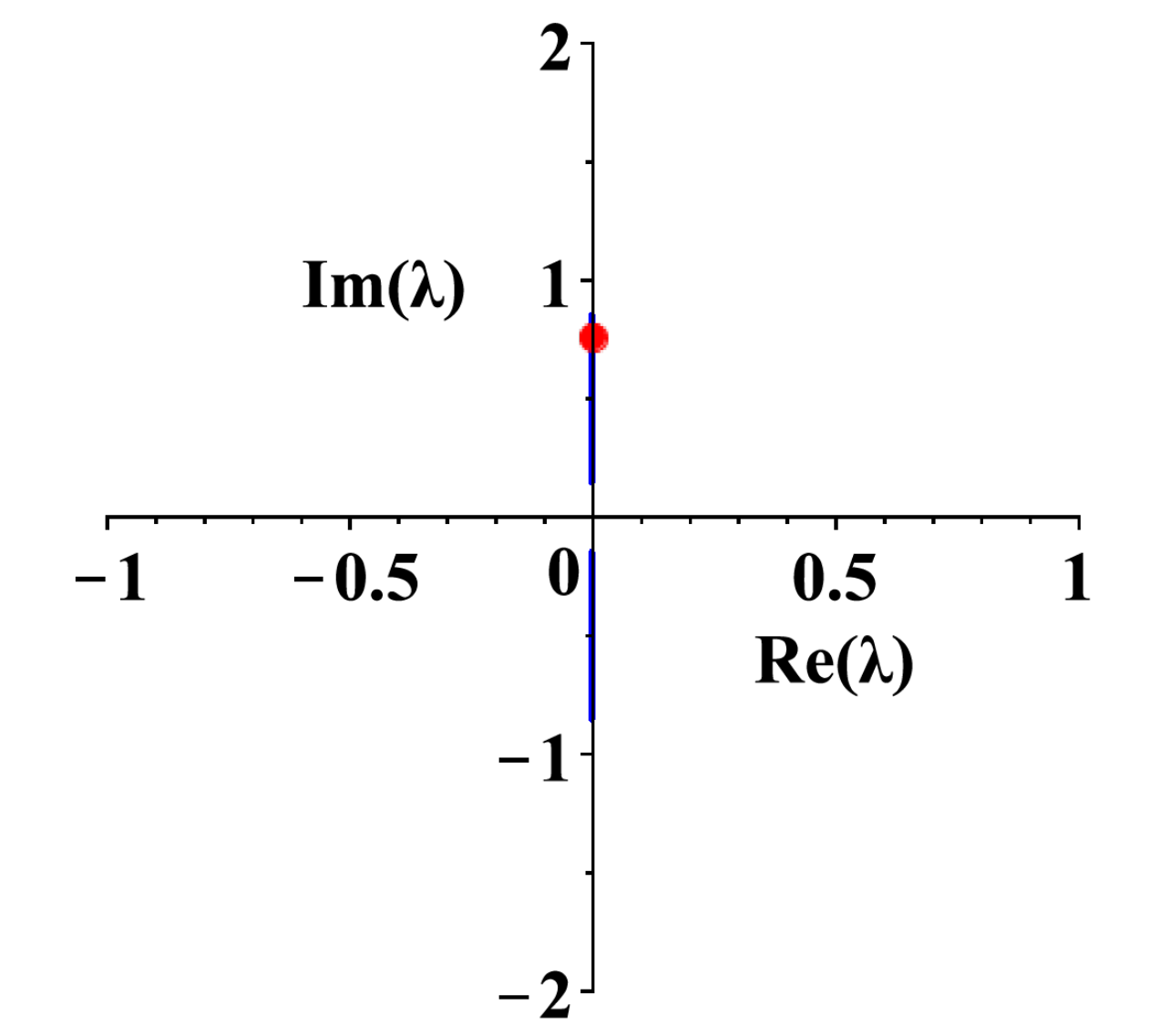
Refer to caption
(a) unstable spectrum in zz plane
Refer to caption
(b) unstable spectrum in λ\lambda plane
Refer to caption
(c) unstable spectrum in Ω\Omega plane
Figure 8. (color online): Unstable dn spectra in z,λ,z,\,\lambda,\, and Ω\Omega plane. The red point represents the parameter used for the plot of the Akhmediev dn breather in Fig. 11.

An interesting application of the above unstable spectra is that we can construct the exact solution to illustrate the modulation dynamics to describe the unstable process. We can obtain such solutions by setting the breather parameter z1z_{1} in one-breather solution [equation (3.7) with n=1n=1] to be values on the lines in Figs. 8-10. Below we provide a few examples.

Let the parameters be k=12k=\frac{1}{\sqrt{2}}, and α=1\alpha=1, l=K′2l=\frac{K^{\prime}}{2}, which infer s2=34s_{2}=\frac{3}{4}. Choosing the parameter z1=−0.527−K⁡(1/2)2​i≈−0.527−0.927​iz_{1}=-0.527-\frac{K(1/2)}{2}\mathrm{i}\approx-0.527-0.927\mathrm{i}, α1=−1\alpha_{1}=-1, we obtain the Akhmediev dn breather (Fig 11 (a)). The maximum value is about 2.3842.384 located at the origin. From the figure 11 (a), we see that there are lots of peaks located on the line t=0t=0, but the value of peaks is less than 2.3842.384, which can be obtained by the analysis of formula (A.2) and is distinct with the Akhmediev breather in the plane wave background. In this setting, it is special that there is no shift of crest under the special parameters setting (Fig 11 (b)), by the above analysis (3.11) and (3.12) for the single breather solution. Here we should point out that this phenomenon with no shift on the crest is a general rule in the dn background. Through the figure 11 (a) and the analysis, we show that this exact breather solution describes the unstable dynamical behavior induced by the unstable spectrum.

Refer to caption
(a) unstable spectrum in zz plane
Refer to caption
(b) unstable spectrum in λ\lambda plane
Refer to caption
(c) unstable spectrum in Ω\Omega plane
Figure 9. (color online): Unstable cn spectra in z,λ,z,\,\lambda,\, and Ω\Omega plane. The red point represents the parameter used for the plot of the Akhmediev cn breather in Fig. 12(a).

Let us set k=12k=\frac{1}{\sqrt{2}}, l=0l=0, and α=1\alpha=1, which implies s2=0s_{2}=0. Choosing the parameters z1≈−0.771−0.560​iz_{1}\approx-0.771-0.560\mathrm{i}, α1=−1\alpha_{1}=-1, we arrive at the Akhmediev cn breather, which admits the phase and crest shift simultaneously (Fig 12 (a)). The maximum value of the peak is about 1.2641.264 located at origin. As the analysis in the above, we know that the other peaks’ value is less than 1.2641.264. In this setting, we can obtain the shift of crest and phase through above general analysis. The dynamics of breather describes the unstable process of the cn solution.

Refer to caption
(a) unstable spectrum in zz plane
Refer to caption
(b) unstable spectrum in λ\lambda plane
Refer to caption
(c) unstable spectrum in Ω\Omega plane
Figure 10. (color online): Unstable spectra in z,λ,z,\,\lambda,\, and Ω\Omega plane for non-trivial phase-modulating background. The red point represents the parameter used for the plot of the Akhmediev breather in Fig. 12(b).

Finally, let us take the parameters k=12k=\frac{1}{\sqrt{2}}, α=1\alpha=1, and l=K⁡(1/2)8l=\frac{K(1/2)}{8}, which yield ν1=−dn2​(K⁡(1/2)+2​i​l)\nu_{1}=-{\rm dn}^{2}(K(1/2)+2\mathrm{i}l), ν2=−12​cn2​(K⁡(1/2)+2​i​l)\nu_{2}=-\frac{1}{2}{\rm cn}^{2}(K(1/2)+2\mathrm{i}l), ν3=12​sn2​(K⁡(1/2)+2​i​l)\nu_{3}=\frac{1}{2}{\rm sn}^{2}(K(1/2)+2\mathrm{i}l) and s2=12​(ν1+ν2+ν3)s_{2}=\frac{1}{2}(\nu_{1}+\nu_{2}+\nu_{3}). Choosing parameters z1=−0.663−0.503​iz_{1}=-0.663-0.503\mathrm{i}, α1=−1\alpha_{1}=-1, we plot Fig. 12 (b). The maximum value of breather is about 1.4141.414 located at origin, which is greater than the other peaks located on the line t=0t=0. This breather describes the unstable dynamics for the elliptic-function background with non-trivial phase modulation.

Refer to caption
(a) Akhmediev dn breather
Refer to caption
(b) asymptotic behavior
Figure 11. (color online): Akhmediev breathers (a) Akhmediev dn breather. (b) The asymptotic behaviors. ψ±\psi_{\pm} represent the different asymptotic behaviors at t=±∞t=\pm\infty.
Refer to caption
(a) Akhmediev cn breather
Refer to caption
(b) Akhmediev non-trivial phase breather
Figure 12. (color online): Akhmediev breathers (a) Akhmediev cn breather. (b) Akhmediev non-trivial phase breather.

5. Rogue waves on the elliptic function background

In this section, we consider the rogue waves, which are located at the branch points. In this case, above two vector solutions (2.36) merge into one vector solution. Thus we need to look for another linear independent vector solution. Here we would like to utilize the limit technique to deal with this problem. Due to the theta function representations include the parameters by Abel map, we still use the original parameter to derive the formulas of rogue waves. Suppose we expand the parameter y⁡(λ)y(\lambda) at the branch point λ1\lambda_{1}: λ=λ1+ϵ12\lambda=\lambda_{1}+\epsilon_{1}^{2}, here ϵ1\epsilon_{1} is a small parameter, then we have the expansions:

(5.1) y⁡(λ)=ϵ1​y1​(1+ϵ12λ1−λ2)​(1+ϵ12λ1−λ3)​(1+ϵ12λ1−λ4)=y1​ϵ1​∑i=0∞y1[i]​ϵ12​i,\begin{split}y(\lambda)&=\epsilon_{1}y_{1}\sqrt{\left(1+\frac{\epsilon_{1}^{2}}{\lambda_{1}-\lambda_{2}}\right)\left(1+\frac{\epsilon_{1}^{2}}{\lambda_{1}-\lambda_{3}}\right)\left(1+\frac{\epsilon_{1}^{2}}{\lambda_{1}-\lambda_{4}}\right)}\\ &=y_{1}\epsilon_{1}\sum_{i=0}^{\infty}y_{1}^{[i]}\epsilon_{1}^{2i},\end{split}

where

y1=(λ1−λ2)​(λ1−λ3)​(λ1−λ4),y1[i]≡(∑l2+l3+l4=i,∏j=24(12lj)(λ1−λj)lj).y_{1}=\sqrt{(\lambda_{1}-\lambda_{2})(\lambda_{1}-\lambda_{3})(\lambda_{1}-\lambda_{4})},\,\,\,\,y_{1}^{[i]}\equiv\left(\sum_{l_{2}+l_{3}+l_{4}=i,}\prod_{j=2}^{4}\frac{\binom{\frac{1}{2}}{l_{j}}}{(\lambda_{1}-\lambda_{j})^{l_{j}}}\right).

It follows that

(5.2) β1​(λ)=2​(λ1+ϵ12)2+s2−2​y​(λ)=2​λ12+s2+2​[ϵ12​(2​λ1+ϵ12)−y1​ϵ1​∑i=0∞y1[i]​ϵ12​i]\begin{split}\beta_{1}(\lambda)&=2(\lambda_{1}+\epsilon_{1}^{2})^{2}+s_{2}-2y(\lambda)\\ &=2\lambda_{1}^{2}+s_{2}+2\left[\epsilon_{1}^{2}(2\lambda_{1}+\epsilon_{1}^{2})-y_{1}\epsilon_{1}\sum_{i=0}^{\infty}y_{1}^{[i]}\epsilon_{1}^{2i}\right]\\ \end{split}

and

(5.3) C1​(λ)=2​λ​β1​(λ)−s3=2​λ13+s2​λ1−s3+2​[ϵ12​[(3​λ12+s2/2)+3​λ1​ϵ12+ϵ14]−y1​ϵ1​(λ1​y1[0]+∑i=1∞(λ1​y1[i]+y1[i−1])​ϵ12​i)].\begin{split}C_{1}(\lambda)&=2\lambda\beta_{1}(\lambda)-s_{3}\\ &=2\lambda_{1}^{3}+s_{2}\lambda_{1}-s_{3}+2\left[\epsilon_{1}^{2}[(3\lambda_{1}^{2}+s_{2}/2)+3\lambda_{1}\epsilon_{1}^{2}+\epsilon_{1}^{4}]-y_{1}\epsilon_{1}\left(\lambda_{1}y_{1}^{[0]}+\sum_{i=1}^{\infty}(\lambda_{1}y_{1}^{[i]}+y_{1}^{[i-1]})\epsilon_{1}^{2i}\right)\right].\end{split}

Moreover, the elements in the vector solution can be expanded in the following:

(5.4) (ν(x)−β1(λ))±1/2=[W1(x)]±1/2(1+K1(ϵ1)+K2(ϵ1))±1/2=[W1(x)]±1/2∑i=0,∞∑j=0i(±12i)(ij)K1i−jK2j=[W1(x)]±1/2∑j=0,∞∑i=0∞(±12i+j)(i+jj)K1iK2j,\begin{split}(\nu(x)-\beta_{1}(\lambda))^{\pm 1/2}&=[W_{1}(x)]^{\pm 1/2}(1+K_{1}(\epsilon_{1})+K_{2}(\epsilon_{1}))^{\pm 1/2}\\ &=[W_{1}(x)]^{\pm 1/2}\sum_{i=0,}^{\infty}\sum_{j=0}^{i}\binom{\pm\frac{1}{2}}{i}\binom{i}{j}K_{1}^{i-j}K_{2}^{j}\\ &=[W_{1}(x)]^{\pm 1/2}\sum_{j=0,}^{\infty}\sum_{i=0}^{\infty}\binom{\pm\frac{1}{2}}{i+j}\binom{i+j}{j}K_{1}^{i}K_{2}^{j},\end{split}

where

W1​(x)=ν⁡(x)−(2​λ12+s2),K1​(ϵ1)=−2​ϵ12​(2​λ1+ϵ12)W1​(x),K2​(ϵ1)=2​y1​ϵ1​∑i=0∞y1[i]​ϵ12​iW1​(x).W_{1}(x)=\nu(x)-(2\lambda_{1}^{2}+s_{2}),\,\,\,\,\,K_{1}(\epsilon_{1})=\frac{-2\epsilon_{1}^{2}(2\lambda_{1}+\epsilon_{1}^{2})}{W_{1}(x)},\,\,\,\,K_{2}(\epsilon_{1})=\frac{2y_{1}\epsilon_{1}{\displaystyle\sum_{i=0}^{\infty}y_{1}^{[i]}\epsilon_{1}^{2i}}}{W_{1}(x)}.

We need the combinatorial formulas:

∑i=0∞(±12i+j)​(i+jj)​K1i=∑i=0∞(±12i+j)​(i+jj)​(−2W1​(x))i​ϵ12​i​(2​λ1+ϵ12)i=∑i=0,∞∑k=0i(12i+j)​(i+jj)​(ik)​(−2W1​(x))i​(2​λ1)i−k​ϵ12​(k+i)=∑k=0,∞∑i=2​k∞(±12i−k+j)​(i−k+jj)​(i−kk)​(−2W1​(x))i−k​(2​λ1)i−2​k​ϵ12​i=∑i=0∞∑k=0[i/2](±12i−k+j)​(i−k+jj)​(i−kk)​(−2W1​(x))i−k​(2​λ1)i−2​k​ϵ12​i\begin{split}\sum_{i=0}^{\infty}\binom{\pm\frac{1}{2}}{i+j}\binom{i+j}{j}K_{1}^{i}=&\sum_{i=0}^{\infty}\binom{\pm\frac{1}{2}}{i+j}\binom{i+j}{j}\left(\frac{-2}{W_{1}(x)}\right)^{i}\epsilon_{1}^{2i}(2\lambda_{1}+\epsilon_{1}^{2})^{i}\\ =&\sum_{i=0,}^{\infty}\sum_{k=0}^{i}\binom{\frac{1}{2}}{i+j}\binom{i+j}{j}\binom{i}{k}\left(\frac{-2}{W_{1}(x)}\right)^{i}(2\lambda_{1})^{i-k}\epsilon_{1}^{2(k+i)}\\ =&\sum_{k=0,}^{\infty}\sum_{i=2k}^{\infty}\binom{\pm\frac{1}{2}}{i-k+j}\binom{i-k+j}{j}\binom{i-k}{k}\left(\frac{-2}{W_{1}(x)}\right)^{i-k}(2\lambda_{1})^{i-2k}\epsilon_{1}^{2i}\\ =&\sum_{i=0}^{\infty}\sum_{k=0}^{[i/2]}\binom{\pm\frac{1}{2}}{i-k+j}\binom{i-k+j}{j}\binom{i-k}{k}\left(\frac{-2}{W_{1}(x)}\right)^{i-k}(2\lambda_{1})^{i-2k}\epsilon_{1}^{2i}\end{split}

and

K2j=(2​y1W1​(x))j​ϵ1j​(∑i=0∞y1[i]​ϵ12​i)j=(2​y1W1​(x))j​ϵ1j​∑n=0∞j!​(∑∑m=0nm​sm=n,∑m=0nsm=j∏m=0n(y1[m])smsm!)​ϵ12​n.\begin{split}K_{2}^{j}=&\left(\frac{2y_{1}}{W_{1}(x)}\right)^{j}\epsilon_{1}^{j}\left(\sum_{i=0}^{\infty}y_{1}^{[i]}\epsilon_{1}^{2i}\right)^{j}\\ =&\left(\frac{2y_{1}}{W_{1}(x)}\right)^{j}\epsilon_{1}^{j}\sum_{n=0}^{\infty}j!\left(\sum_{\sum_{m=0}^{n}ms_{m}=n,}^{\sum_{m=0}^{n}s_{m}=j}\prod_{m=0}^{n}\frac{\left(y_{1}^{[m]}\right)^{s_{m}}}{s_{m}!}\right)\epsilon_{1}^{2n}.\end{split}

Let us introduce the notation

Gi,j±≡∑k=0[i/2](±12i−k+j)​(i−k+jj)​(i−kk)​(−2W1​(x))i−k​(2​λ1)i−2​kG^{\pm}_{i,j}\equiv\sum_{k=0}^{[i/2]}\binom{\pm\frac{1}{2}}{i-k+j}\binom{i-k+j}{j}\binom{i-k}{k}\left(\frac{-2}{W_{1}(x)}\right)^{i-k}(2\lambda_{1})^{i-2k}

and

Hn,j=j!​(∑∑m=0nm​sm=n,∑m=0nsm=j∏m=0n(y1[m])smsm!),H_{n,j}=j!\left(\sum_{\sum_{m=0}^{n}ms_{m}=n,}^{\sum_{m=0}^{n}s_{m}=j}\prod_{m=0}^{n}\frac{\left(y_{1}^{[m]}\right)^{s_{m}}}{s_{m}!}\right),

then we arrive at

(5.5) (ν(x)−β1(λ))±1/2=[W1(x)]±1/2∑j=0∞(2​y1W1​(x))jϵ1j∑k=0∞(∑i+n=kG±i,jHn,j)ϵ12​k=[W1(x)]±1/2∑k=0,∞∑j=0∞(2​y1W1​(x))j(∑i+n=kG±i,jHn,j)ϵ12​k+j=[W1(x)]±1/2∑k=0,∞∑j=2​k∞(2​y1W1​(x))j−2​k(∑i+n=kG±i,j−2​kHn,j−2​k)ϵ1j=[W1(x)]±1/2∑j=0∞[∑k=0[j/2](2​y1W1​(x))j−2​k(∑i+n=kG±i,j−2​kHn,j−2​k)]ϵ1j≡[W1(x)]±1/2∑j=0∞ν1±[j]ϵ1j,\begin{split}(\nu(x)-\beta_{1}(\lambda))^{\pm 1/2}&=[W_{1}(x)]^{\pm 1/2}\sum_{j=0}^{\infty}\left(\frac{2y_{1}}{W_{1}(x)}\right)^{j}\epsilon_{1}^{j}\sum_{k=0}^{\infty}\left(\sum_{i+n=k}G^{\pm}_{i,j}H_{n,j}\right)\epsilon_{1}^{2k}\\ &=[W_{1}(x)]^{\pm 1/2}\sum_{k=0,}^{\infty}\sum_{j=0}^{\infty}\left(\frac{2y_{1}}{W_{1}(x)}\right)^{j}\left(\sum_{i+n=k}G^{\pm}_{i,j}H_{n,j}\right)\epsilon_{1}^{2k+j}\\ &=[W_{1}(x)]^{\pm 1/2}\sum_{k=0,}^{\infty}\sum_{j=2k}^{\infty}\left(\frac{2y_{1}}{W_{1}(x)}\right)^{j-2k}\left(\sum_{i+n=k}G^{\pm}_{i,j-2k}H_{n,j-2k}\right)\epsilon_{1}^{j}\\ &=[W_{1}(x)]^{\pm 1/2}\sum_{j=0}^{\infty}\left[\sum_{k=0}^{[j/2]}\left(\frac{2y_{1}}{W_{1}(x)}\right)^{j-2k}\left(\sum_{i+n=k}G^{\pm}_{i,j-2k}H_{n,j-2k}\right)\right]\epsilon_{1}^{j}\\ &\equiv[W_{1}(x)]^{\pm 1/2}\sum_{j=0}^{\infty}\nu_{1\pm}^{[j]}\epsilon_{1}^{j},\end{split}

where [⋅][\cdot] represents the floor function. In a similar fashion, we get the expansion for 1/(ν⁡(x)−β1​(λ))1/(\nu(x)-\beta_{1}(\lambda)):

(5.6) (ν⁡(x)−β1​(λ))−1=[W1​(x)]−1​∑j=0∞Rj​ϵ1j,(\nu(x)-\beta_{1}(\lambda))^{-1}=[W_{1}(x)]^{-1}\sum_{j=0}^{\infty}R_{j}\epsilon_{1}^{j},

where we have defined

(5.7) Rj\displaystyle R_{j} ≡∑k=0[j/2](2​y1W1​(x))j−2​k​(∑i+n=kGi,j−2​k′​Hn,j−2​k),\displaystyle\equiv\sum_{k=0}^{[j/2]}\left(\frac{2y_{1}}{W_{1}(x)}\right)^{j-2k}\left(\sum_{i+n=k}G^{\prime}_{i,j-2k}H_{n,j-2k}\right),
(5.8) Gi,j′\displaystyle G^{\prime}_{i,j} ≡∑k=0[i/2](−1)i−k+j​(i−k+jj)​(i−kk)​(−2W1​(x))i−k​(2​λ1)i−2​k.\displaystyle\equiv\sum_{k=0}^{[i/2]}(-1)^{i-k+j}\binom{i-k+j}{j}\binom{i-k}{k}\left(\frac{-2}{W_{1}(x)}\right)^{i-k}(2\lambda_{1})^{i-2k}.

With the help of equations (5.3) and (5.6), it follows that

(5.9) C1(ν⁡(x)−β1​(λ))=C1W1​(x)​∑j=0∞Rj​ϵ1j=1W1​(x)∑j=0∞[(2λ13+s2λ1−s3)Rj−2λ1y1y1[0]Rj−1χ[j≥1]+2(3λ12+s22)Rj−2χ[j≥2]−2y1(∑i=0[(j−3)/2](λ1y1[i+1]+y1[i])Rj−3−2​i)χ[j≥3]+6λ1Rj−4χ[j≥4]+2Rj−6χ[j≥6]]ϵ1j≡∑j=0∞Ij​(x)​ϵ1j,\begin{split}\frac{C_{1}}{(\nu(x)-\beta_{1}(\lambda))}&=\frac{C_{1}}{W_{1}(x)}\sum_{j=0}^{\infty}R_{j}\epsilon_{1}^{j}\\ &=\frac{1}{W_{1}(x)}\sum_{j=0}^{\infty}\left[(2\lambda_{1}^{3}+s_{2}\lambda_{1}-s_{3})R_{j}-2\lambda_{1}y_{1}y_{1}^{[0]}R_{j-1}\chi_{[j\geq 1]}+2\left(3\lambda_{1}^{2}+\frac{s_{2}}{2}\right)R_{j-2}\chi_{[j\geq 2]}\right.\\ &\,\,\,\,\,\,\,\left.-2y_{1}\left(\sum_{i=0}^{[(j-3)/2]}(\lambda_{1}y_{1}^{[i+1]}+y_{1}^{[i]})R_{j-3-2i}\right)\chi_{[j\geq 3]}+6\lambda_{1}R_{j-4}\chi_{[j\geq 4]}+2R_{j-6}\chi_{[j\geq 6]}\right]\epsilon_{1}^{j}\\ &\equiv\sum_{j=0}^{\infty}I_{j}(x)\epsilon_{1}^{j},\end{split}

where

χ[j≥s]={1,j≥s0,j<s.\chi_{[j\geq s]}=\left\{\begin{matrix}1,&j\geq s\\ 0,&j<s.\end{matrix}\right.

Then we obtain the expansion for the phase factor:

(5.10) θ1​(λ)=i​∫0xC1​d​sν⁡(s)−β1+i​λ​x+i⁡(s22+y)​t=i⁡[∫0xI0​(s)​ds+λ1​x+s22​t+∑j=1∞(∫0xIj​(s)​ds)​ϵ1j+x​ϵ12+y1​∑i=0∞y1[i]​t​ϵ12​i+1]≡∑i=0∞Θ1[i]​ϵ1i.\begin{split}\theta_{1}(\lambda)&=\mathrm{i}\int_{0}^{x}\frac{C_{1}{\rm d}s}{\nu(s)-\beta_{1}}+\mathrm{i}\lambda x+\mathrm{i}(\frac{s_{2}}{2}+y)t\\ &=\mathrm{i}\left[\int_{0}^{x}I_{0}(s){\rm d}s+\lambda_{1}x+\frac{s_{2}}{2}t+\sum_{j=1}^{\infty}\left(\int_{0}^{x}I_{j}(s){\rm d}s\right)\epsilon_{1}^{j}+x\epsilon_{1}^{2}+y_{1}\sum_{i=0}^{\infty}y_{1}^{[i]}t\epsilon_{1}^{2i+1}\right]\\ &\equiv\sum_{i=0}^{\infty}\Theta_{1}^{[i]}\epsilon_{1}^{i}.\end{split}
Remark 4.

Here we point out that the integrations ∫0xIj​(s)​𝑑s,\int_{0}^{x}I_{j}(s){\rm d}s, (i≥1)(i\geq 1) do not possess integrals of the third kind. In general, the integration ∫0xIj​(s)​𝑑s\int_{0}^{x}I_{j}(s){\rm d}s can be expressed in terms of elliptic functions and elliptic integrals of the second and third kind via the formulas (B.1),(B.2) and (B.3). It is hard to give a claim that the integrations ∫0xIj​(s)​𝑑s,\int_{0}^{x}I_{j}(s){\rm d}s, (i≥1)(i\geq 1) do not have the elliptic integral of the third by the pure algebraic calculations. It is much easier to give a proof by analyzing the singularity point at the point x=ξmodΛ∈{2mK+niK′|m,n∈ℤ}x=\xi\mod\Lambda\in\{2mK+n\mathrm{i}\,K^{\prime}|m,n\in\mathbb{Z}\} when ν⁡(ξ)−(2​λ12+s2)=0\nu(\xi)-(2\lambda_{1}^{2}+s_{2})=0. By using the conformal transformation (2.43) and (2.44), the integration

i​∫0xC1​d​sν⁡(s)−β1=i2​∫0α​xdd​z​sn2​(i⁡(z−l))​d​ssn2​(i⁡(z−l))−sn2​(s)\mathrm{i}\int_{0}^{x}\frac{C_{1}\,{\rm d}s}{\nu(s)-\beta_{1}}=\frac{\mathrm{i}}{2}\int_{0}^{\alpha\,x}\frac{\frac{{\rm d}}{{\rm d}z}{\rm sn}^{2}(\mathrm{i}(z-l))\,{\rm d}s}{{\rm sn}^{2}(\mathrm{i}(z-l))-{\rm sn}^{2}(s)}

has the logarithmic singularity at x=ξmodΛx=\xi\mod\Lambda. Expanding the above integration at λ=λ1\lambda=\lambda_{1} is equivalent to the expansion at z=zs≡K′+i​K2=−i⁡(α​ξ+z0).z=z_{s}\equiv\frac{K^{\prime}+\mathrm{i}K}{2}=-\mathrm{i}(\alpha\,\xi+z_{0}). Firstly, we have the following two expansions:

sn2​(i⁡(z−l))−sn2​(s)=∑i=1∞[(dii!​d​zi​sn2​(i⁡(z−l)))|z=zs​[(z−zs)i−(i​α​ξ−i​s)i]],{\rm sn}^{2}(\mathrm{i}(z-l))-{\rm sn}^{2}(s)=\sum_{i=1}^{\infty}\left[\left(\frac{{\rm d}^{i}}{i!{\rm d}z^{i}}{\rm sn}^{2}(\mathrm{i}(z-l))\right)|_{z=z_{s}}[(z-z_{s})^{i}-(\mathrm{i}\alpha\xi-\mathrm{i}s)^{i}]\right],

and

dd​z​sn2​(i⁡(z−l))=∑i=1∞(di(i−1)!​d​zi​sn2​(i⁡(z−l)))|z=zs​(z−zs)i−1.\frac{{\rm d}}{{\rm d}z}{\rm sn}^{2}(\mathrm{i}(z-l))=\sum_{i=1}^{\infty}\left(\frac{{\rm d}^{i}}{(i-1)!{\rm d}z^{i}}{\rm sn}^{2}(\mathrm{i}(z-l))\right)|_{z=z_{s}}(z-z_{s})^{i-1}.

Thus we have

∫i2​dd​z​sn2​(i⁡(z−l))​d​ssn2​(i⁡(z−l))−sn2​(s)=12​ln⁡(s−α​ξ)+O⁡(z−zs)O⁡(s−α​ξ),\int\frac{\mathrm{i}}{2}\frac{\frac{{\rm d}}{{\rm d}z}{\rm sn}^{2}(\mathrm{i}(z-l)){\rm d}s}{{\rm sn}^{2}(\mathrm{i}(z-l))-{\rm sn}^{2}(s)}=\frac{1}{2}\ln(s-\alpha\xi)+\frac{O(z-z_{s})}{O(s-\alpha\xi)},

which infers that the logarithmic singularity can not appear at the higher-order term of (z−zs).(z-z_{s}). Moreover, the higher-order terms of (z−zs)(z-z_{s}) do not involve elliptic integrals of the third kind since the leading order term involves the logarithmic singularity. From the conformal transformation

α​∫0λd​μ(μ−λ1)​(μ−λ1∗)​(μ−λ2)​(μ−λ2∗)=2​(z−l).\alpha\int_{0}^{\lambda}\frac{{\rm d}\mu}{\sqrt{(\mu-\lambda_{1})(\mu-\lambda_{1}^{*})(\mu-\lambda_{2})(\mu-\lambda_{2}^{*})}}=2(z-l).

we can deduce that, at the critical point z=zsz=z_{s}, we have the expansion λ⁡(z)−λ1=(z−zs)2​H2​(z−zs)\lambda(z)-\lambda_{1}=(z-z_{s})^{2}H^{2}(z-z_{s}), where H⁡(z−zs)H(z-z_{s}) is an analytic function with H⁡(0)≠0.H(0)\neq 0. So ϵ1=(z−zs)​H​(z−zs)\epsilon_{1}=(z-z_{s})H(z-z_{s}) and

∫C1​d​sν⁡(s)−β1=12​ln⁡(s−α​ξ)+O⁡(ϵ1)O⁡(s−α​ξ),\int\frac{C_{1}{\rm d}s}{\nu(s)-\beta_{1}}=\frac{1}{2}\ln(s-\alpha\xi)+\frac{O(\epsilon_{1})}{O(s-\alpha\xi)},

which implies that there appears no elliptic integral of the third kind in the coefficients of higher-order terms of ϵ1\epsilon_{1}.

By the Schur polynomial, we have

exp⁡[θ1]=exp⁡[Θ1[0]]​∑i=0∞E1[i]​ϵ1i,\exp[\theta_{1}]=\exp[\Theta_{1}^{[0]}]\sum_{i=0}^{\infty}E_{1}^{[i]}\epsilon_{1}^{i},

where

E1[i]=∑∑k=1mk​lk=i(∏j=1m(Θ1[j])ljlj!).E_{1}^{[i]}=\sum_{\sum_{k=1}^{m}kl_{k}=i}\left(\prod_{j=1}^{m}\frac{(\Theta_{1}^{[j]})^{l_{j}}}{l_{j}!}\right).

Summarizing, we obtain the expansion for the first component of vector solution:

ν​(x)−β1​(λ)​exp⁡(θ1)=W1​(x)​exp⁡[Θ1[0]]​∑i=0∞ϕ1[i]​ϵ1i,ϕ1[i]=∑j=0iE1[j]​ν1+[i−j].\sqrt{\nu(x)-\beta_{1}(\lambda)}\exp(\theta_{1})=\sqrt{W_{1}(x)}\exp[\Theta_{1}^{[0]}]\sum_{i=0}^{\infty}\phi_{1}^{[i]}\epsilon_{1}^{i},\,\,\,\,\,\phi_{1}^{[i]}=\sum_{j=0}^{i}E_{1}^{[j]}\nu_{1+}^{[i-j]}.

To derive the expansion for the second component, we need to expand the following expression:

r1=i​hf−y=2​ψ∗​λ−i​ψx∗ν​(x)−β1​(λ)=2​ν​(x)​λ1−i⁡(νx​(x)/2+i​q)+2​ν​(x)​ϵ12ν⁡(x)​(ν⁡(x)−β1​(λ))​exp⁡[i​q​∫0xd​sν⁡(s)−i​s2​t].r_{1}=\frac{\mathrm{i}h}{f-y}=\frac{2\psi^{*}\lambda-\mathrm{i}\psi^{*}_{x}}{\nu(x)-\beta_{1}(\lambda)}=\frac{2\nu(x)\lambda_{1}-\mathrm{i}(\nu_{x}(x)/2+\mathrm{i}q)+2\nu(x)\epsilon_{1}^{2}}{\sqrt{\nu(x)}(\nu(x)-\beta_{1}(\lambda))}\exp\left[\mathrm{i}q\int_{0}^{x}\frac{{\rm d}s}{\nu(s)}-\mathrm{i}s_{2}t\right].

In fact, the second component of the vector solution has the expansion

2​ν​(x)​λ1−i⁡(νx​(x)/2+i​q)+2​ν​(x)​ϵ12ν⁡(x)​exp⁡(θ1)ν​(x)−β1​(λ)​exp⁡[i​q​∫0xd​sν⁡(s)−i​s2​t]=exp⁡[i​q​∫0xd​sν⁡(s)−i​s2​t]​ν⁡(x)​exp⁡[Θ1[0]]W1​(x)​∑i=0∞φ1[i]​ϵ1i,\begin{split}&\frac{2\nu(x)\lambda_{1}-\mathrm{i}(\nu_{x}(x)/2+\mathrm{i}q)+2\nu(x)\epsilon_{1}^{2}}{\sqrt{\nu(x)}}\frac{\exp(\theta_{1})}{\sqrt{\nu(x)-\beta_{1}(\lambda)}}\exp\left[\mathrm{i}q\int_{0}^{x}\frac{{\rm d}s}{\nu(s)}-\mathrm{i}s_{2}t\right]\\ =&\exp\left[\mathrm{i}q\int_{0}^{x}\frac{{\rm d}s}{\nu(s)}-\mathrm{i}s_{2}t\right]\frac{\sqrt{\nu(x)}\exp[\Theta_{1}^{[0]}]}{\sqrt{W_{1}(x)}}\sum_{i=0}^{\infty}\varphi_{1}^{[i]}\epsilon_{1}^{i},\end{split}

where

φ1[i]=2​ν​(x)​λ1−i⁡(νx​(x)/2+i​q)ν⁡(x)∑j=0iE1[j]ν1−[i−j]+2χ[i≥2]∑j=0i−2E1[j]ν1−[i−2−j].\varphi_{1}^{[i]}=\frac{2\nu(x)\lambda_{1}-\mathrm{i}(\nu_{x}(x)/2+\mathrm{i}q)}{\nu(x)}\sum_{j=0}^{i}E_{1}^{[j]}\nu_{1-}^{[i-j]}+2\chi_{[i\geq 2]}\sum_{j=0}^{i-2}E_{1}^{[j]}\nu_{1-}^{[i-2-j]}.

In a similar procedure, we obtain the expansion at λ=λ2\lambda=\lambda_{2}:

ν​(x)−β1​(λ)​exp⁡(θ1)=W1​(x)​exp⁡[Θ2[0]]​∑i=0∞ϕ2[i]​ϵ2i,r1​ν​(x)−β1​(λ)​exp⁡(θ1)=exp⁡[i​q​∫0xd​sν⁡(s)−i​s2​t]​ν⁡(x)​exp⁡[Θ2[0]]W1​(x)​∑i=0∞φ2[i]​ϵ2i,\begin{split}\sqrt{\nu(x)-\beta_{1}(\lambda)}\exp(\theta_{1})&=\sqrt{W_{1}(x)}\exp[\Theta_{2}^{[0]}]\sum_{i=0}^{\infty}\phi_{2}^{[i]}\epsilon_{2}^{i},\\ r_{1}\sqrt{\nu(x)-\beta_{1}(\lambda)}\exp(\theta_{1})&=\exp\left[\mathrm{i}q\int_{0}^{x}\frac{{\rm d}s}{\nu(s)}-\mathrm{i}s_{2}t\right]\frac{\sqrt{\nu(x)}\exp[\Theta_{2}^{[0]}]}{\sqrt{W_{1}(x)}}\sum_{i=0}^{\infty}\varphi_{2}^{[i]}\epsilon_{2}^{i},\end{split}

where Θ2[i]\Theta_{2}^{[i]}, ϕ2[i]\phi_{2}^{[i]} and φ2[i]\varphi_{2}^{[i]} are Θ1[i]\Theta_{1}^{[i]}, ϕ1[i]\phi_{1}^{[i]} and φ1[i]\varphi_{1}^{[i]} by exchanging the variables λ1\lambda_{1} to λ2.\lambda_{2}. By the Remark 4 and the integration formulas (B.1), (B.2) and (B.3), we know that the functions ϕk[i]\phi_{k}^{[i]}, φk[i]\varphi_{k}^{[i]} (k=1,2;i∈ℤ+k=1,2;i\in\mathbb{Z}^{+}) are the rational function of sn\mathrm{sn}, cn\mathrm{cn}, dn\mathrm{dn} and the second type of elliptic integration E⁡(u)E(u).

Summarizing the above, we can obtain the following theorem of rogue waves:

Theorem 5.

The general rogue wave formulas obtained by the high order Darboux transformation (in the Appendix A) can be represented as

(5.11) ψn1,n2=ν⁡(x)[det(𝐊n)det(𝐌n)]exp[−iq∫0xd​sν⁡(s)+is2t],\psi_{n_{1},n_{2}}=\sqrt{\nu(x)}\left[\frac{\det(\mathbf{K}_{n})}{\det(\mathbf{M}_{n})}\right]\exp\left[-\mathrm{i}q\int_{0}^{x}\frac{{\rm d}s}{\nu(s)}+\mathrm{i}s_{2}t\right],

where 𝐌n=ν⁡(x)​𝐗n†​𝐃n​𝐗n+𝐘n†​𝐃n​𝐘n\mathbf{M}_{n}=\nu(x)\mathbf{X}_{n}^{{\dagger}}\mathbf{D}_{n}\mathbf{X}_{n}+\mathbf{Y}_{n}^{{\dagger}}\mathbf{D}_{n}\mathbf{Y}_{n}, 𝐊n=𝐌n−2​𝐗n,1†​𝐘n,1\mathbf{K}_{n}=\mathbf{M}_{n}-2\mathbf{X}_{n,1}^{{\dagger}}\mathbf{Y}_{n,1}, 𝐗n,1=[𝐗1[1],𝐗1[2]]\mathbf{X}_{n,1}=[\mathbf{X}_{1}^{[1]},\mathbf{X}_{1}^{[2]}], 𝐘n,1=[𝐘1[1],𝐘1[2]]\mathbf{Y}_{n,1}=[\mathbf{Y}_{1}^{[1]},\mathbf{Y}_{1}^{[2]}] and

𝐃n=[𝐃[1,1]𝐃[1,2]𝐃[2,1]𝐃[2,2]],𝐃[l,k]=((i+j−2i−1)​(−1)j−1(λk−λl∗)i+j−1)1≤i≤nl,0≤j≤nk,\mathbf{D}_{n}=\begin{bmatrix}\mathbf{D}^{[1,1]}&\mathbf{D}^{[1,2]}\\ \mathbf{D}^{[2,1]}&\mathbf{D}^{[2,2]}\\ \end{bmatrix},\,\,\,\,\,\mathbf{D}^{[l,k]}=\left(\binom{i+j-2}{i-1}\frac{(-1)^{j-1}}{(\lambda_{k}-\lambda_{l}^{*})^{i+j-1}}\right)_{1\leq i\leq n_{l},0\leq j\leq n_{k}},
𝐗n=[𝐗[1]00𝐗[2]],𝐘n=[𝐘[1]00𝐘[2]],\mathbf{X}_{n}=\begin{bmatrix}\mathbf{X}^{[1]}&0\\ 0&\mathbf{X}^{[2]}\\ \end{bmatrix},\,\,\,\,\,\mathbf{Y}_{n}=\begin{bmatrix}\mathbf{Y}^{[1]}&0\\ 0&\mathbf{Y}^{[2]}\\ \end{bmatrix},

and l,k=1,2l,k=1,2, n1+n2=n,n_{1}+n_{2}=n,

𝐗[l]=[φl[1]φl[3]φl[5]⋯φl[2​nl−1]0φl[1]φl[3]⋯φl[2​nl−3]000⋯φl[1]],𝐘[l]=(ν⁡(x)−(2​λl2+s2))​[ϕl[1]ϕl[3]ϕl[5]⋯ϕl[2​nl−1]0ϕl[1]ϕl[3]⋯ϕl[2​nl−3]000⋯ϕl[1]],\mathbf{X}^{[l]}=\begin{bmatrix}\varphi_{l}^{[1]}&\varphi_{l}^{[3]}&\varphi_{l}^{[5]}&\cdots&\varphi_{l}^{[2n_{l}-1]}\\[8.0pt] 0&\varphi_{l}^{[1]}&\varphi_{l}^{[3]}&\cdots&\varphi_{l}^{[2n_{l}-3]}\\ \vdots&\vdots&\vdots&&\vdots\\ 0&0&0&\cdots&\varphi_{l}^{[1]}\\ \end{bmatrix},\,\,\,\,\mathbf{Y}^{[l]}=(\nu(x)-(2\lambda_{l}^{2}+s_{2}))\begin{bmatrix}\phi_{l}^{[1]}&\phi_{l}^{[3]}&\phi_{l}^{[5]}&\cdots&\phi_{l}^{[2n_{l}-1]}\\[8.0pt] 0&\phi_{l}^{[1]}&\phi_{l}^{[3]}&\cdots&\phi_{l}^{[2n_{l}-3]}\\ \vdots&\vdots&\vdots&&\vdots\\ 0&0&0&\cdots&\phi_{l}^{[1]}\\ \end{bmatrix},

and 𝐗1[l]\mathbf{X}_{1}^{[l]} and 𝐘1[l]\mathbf{Y}_{1}^{[l]} represent the first row of 𝐗[l]\mathbf{X}^{[l]} and 𝐘[l]\mathbf{Y}^{[l]}, respectively.

The general expressions for the high order rogue waves are very complicated. However, the extremal value at the point (x,t)=(0,0)(x,t)=(0,0) can be obtained through the determinant formula. Since the NLSE possesses the scaling symmetry, we set the amplitude for the background be 11: i.e., ν3=1\nu_{3}=1 without loss of generality. Then, the vector fundamental solution at (x,t)=(0,0)(x,t)=(0,0) can be written as

[ϕ1​(0,0,λ)φ1​(0,0,λ)]=[ν3−2​(λ2+s2/2−y)i​ν3−2​(λ2+s2/2+y)].\begin{bmatrix}\phi_{1}(0,0;\lambda)\\[5.0pt] \varphi_{1}(0,0;\lambda)\\ \end{bmatrix}=\begin{bmatrix}\sqrt{\nu_{3}-2(\lambda^{2}+s_{2}/2-y)}\\[5.0pt] \mathrm{i}\sqrt{\nu_{3}-2(\lambda^{2}+s_{2}/2+y)}\\ \end{bmatrix}.

At the branch points λ=λi+ϵi2\lambda=\lambda_{i}+\epsilon_{i}^{2}, we know that y⁡(−ϵi)=−y⁡(ϵi)y(-\epsilon_{i})=-y(\epsilon_{i}), i=1,2i=1,2. So we have the expansion

[ϕ1​(0,0,λ)φ1​(0,0,λ)]=∑j=0∞[ϕ1[j]​(0,0,λi)i​(−1)i​ϕ1[j]​(0,0,λi)]ϵij,i=1,2.\begin{bmatrix}\phi_{1}(0,0;\lambda)\\[5.0pt] \varphi_{1}(0,0;\lambda)\\ \end{bmatrix}=\sum_{j=0}^{\infty}\begin{bmatrix}\phi_{1}^{[j]}(0,0;\lambda_{i})\\[5.0pt] \mathrm{i}(-1)^{i}\phi_{1}^{[j]}(0,0;\lambda_{i})\\ \end{bmatrix}\epsilon_{i}^{j},\,\,\,\,\,i=1,2.

Moreover, we have

ψn​(0,0)=det(𝐌n−i​𝐗n,1†​𝐗n,1)det(𝐌n),\psi_{n}(0,0)=\frac{\det(\mathbf{M}_{n}-\mathrm{i}\mathbf{X}_{n,1}^{{\dagger}}\mathbf{X}_{n,1})}{\det(\mathbf{M}_{n})},

where 𝐌n=𝐗n†​𝐃n​𝐗n\mathbf{M}_{n}=\mathbf{X}_{n}^{{\dagger}}\mathbf{D}_{n}\mathbf{X}_{n}, 𝐗1,n=[ϕ1[1]​(λ1),ϕ1[3]​(λ1),⋯,ϕ1[2​n1−1]​(λ1),ϕ1[1]​(λ2),ϕ1[3]​(λ2),⋯,ϕ1[2​n2−1]​(λ2)],\mathbf{X}_{1,n}=[\phi_{1}^{[1]}(\lambda_{1}),\phi_{1}^{[3]}(\lambda_{1}),\cdots,\phi_{1}^{[2n_{1}-1]}(\lambda_{1}),\phi_{1}^{[1]}(\lambda_{2}),\phi_{1}^{[3]}(\lambda_{2}),\cdots,\phi_{1}^{[2n_{2}-1]}(\lambda_{2})], and

𝐗n=[𝐗[1]00𝐗[2]],𝐗[i]=[ϕ1[1]​(λi)ϕ1[3]​(λi)⋯ϕ1[2​n1−1]​(λi)0ϕ1[1]​(λi)⋯ϕ1[2​n1−3]​(λi)000ϕ1[1]​(λi)],i=1,2.\mathbf{X}_{n}=\begin{bmatrix}\mathbf{X}^{[1]}&0\\ 0&\mathbf{X}^{[2]}\\ \end{bmatrix},\,\,\,\,\,\,\mathbf{X}^{[i]}=\begin{bmatrix}\phi_{1}^{[1]}(\lambda_{i})&\phi_{1}^{[3]}(\lambda_{i})&\cdots&\phi_{1}^{[2n_{1}-1]}(\lambda_{i})\\ 0&\phi_{1}^{[1]}(\lambda_{i})&\cdots&\phi_{1}^{[2n_{1}-3]}(\lambda_{i})\\ &&&\\ 0&0&0&\phi_{1}^{[1]}(\lambda_{i})\\ \end{bmatrix},\,\,\,\,\,i=1,2.

By the formula of the Cauchy determinant and taking its special limit, we find

ψn​(0,0)=det(𝐃^n)det(𝐃n)=1+2​(n1​Im​(λ1)+n2​Im​(λ2)),\psi_{n}(0,0)=\frac{\det(\widehat{\mathbf{D}}_{n})}{\det(\mathbf{D}_{n})}=1+2(n_{1}{\rm Im}(\lambda_{1})+n_{2}{\rm Im}(\lambda_{2})),

where

𝐃^n=[𝐃^[1,1]𝐃^[1,2]𝐃^[2,1]𝐃^[2,2]],𝐃^[l,k]=((i+j−2i−1)​(−1)i−1(λk−λl∗)i+j−1−i​δ1,1)1≤i≤nl,0≤j≤nk,\widehat{\mathbf{D}}_{n}=\begin{bmatrix}\widehat{\mathbf{D}}^{[1,1]}&\widehat{\mathbf{D}}^{[1,2]}\\ \widehat{\mathbf{D}}^{[2,1]}&\widehat{\mathbf{D}}^{[2,2]}\\ \end{bmatrix},\,\,\,\,\,\widehat{\mathbf{D}}^{[l,k]}=\left(\binom{i+j-2}{i-1}\frac{(-1)^{i-1}}{(\lambda_{k}-\lambda_{l}^{*})^{i+j-1}}-\mathrm{i}\delta_{1,1}\right)_{1\leq i\leq n_{l},0\leq j\leq n_{k}},

and 1≤l,k≤21\leq l,k\leq 2, δ1,1=1\delta_{1,1}=1 if i=j=1i=j=1, otherwise δ1,1=0.\delta_{1,1}=0.

Here we stress that the high order rogue waves given previously do not possess the free parameters. Actually, since the fundamental solution can involve lots of free parameters, it is easy to bring the free parameters into the formulas of rogue waves as in reference [21].

Now we consider the several explicit examples of the rogue waves. Firstly, we consider the first order rogue wave. We fix the parameters λ1=b+c​i\lambda_{1}=b+c\mathrm{i}, λ2=−b+d​i\lambda_{2}=-b+d\mathrm{i}, λ3=λ1∗\lambda_{3}=\lambda_{1}^{*} and λ4=λ2∗\lambda_{4}=\lambda_{2}^{*}. Using the above expansion, we can obtain that

(5.12) φ1=u1​(x)​p​(x)​exp⁡(θ1​(x,t)),θ1​(x,t)=i​∫0xd​su1​(s)+i​λ1​x+i​s22​tϕ1=ν⁡(x)​u1​(x)​(λ12+(s2−ν⁡(x))/2)​p​(x)+1λ1​ν​(x)+(2​q+i​νx​(x))/4​exp⁡(θ1​(x,t)+i​θ0​(x,t)),\begin{split}\varphi_{1}&=\sqrt{u_{1}(x)}p(x)\exp\left(\theta_{1}(x,t)\right),\,\,\,\,\,\,\theta_{1}(x,t)=\mathrm{i}\int_{0}^{x}\frac{{d}s}{u_{1}(s)}+\mathrm{i}\lambda_{1}x+\mathrm{i}\frac{s_{2}}{2}t\\ \phi_{1}&=\sqrt{\nu(x)}\sqrt{u_{1}(x)}\frac{(\lambda_{1}^{2}+(s_{2}-\nu(x))/2)p(x)+1}{\lambda_{1}\nu(x)+(2q+\mathrm{i}\nu_{x}(x))/4}\exp\left(\theta_{1}(x,t)+\mathrm{i}\theta_{0}(x,t)\right),\end{split}

where θ0​(x,t)=q​∫0xd​sν⁡(s)−s2​t\theta_{0}(x,t)=q\int_{0}^{x}\frac{{d}s}{\nu(s)}-s_{2}t, p⁡(x)=1u1​(x)+i​t+J⁡(x)+k1p(x)=\frac{1}{u_{1}(x)}+\mathrm{i}t+J(x)+k_{1}, u1​(x)=ν⁡(x)−(2​λ12+s2)u_{1}(x)=\nu(x)-(2\lambda_{1}^{2}+s_{2}), C1=2​λ1​(2​λ12+s2)−s3C_{1}=2\lambda_{1}(2\lambda_{1}^{2}+s_{2})-s_{3}, k1∈ℂk_{1}\in\mathbb{C}, and the integration

J⁡(x)=−4iλ1∫0xd​su1​(s)−2iC1∫0xd​su12​(s)=A1​(EK​α​x+Z⁡(α​x))+A2​x+A3​sn⁡(α​x)​cn​(α​x)​dn​(α​x)u1​(x),\begin{split}J(x)&=-4\mathrm{i}\lambda_{1}\int_{0}^{x}\frac{{d}s}{u_{1}(s)}-2\mathrm{i}C_{1}\int_{0}^{x}\frac{{d}s}{u_{1}^{2}(s)}\\ &=A_{1}\left(\frac{E}{K}\alpha\,x+Z(\alpha\,x)\right)+A_{2}x+A_{3}\frac{{\rm sn}(\alpha\,x){\rm cn}(\alpha\,x){\rm dn}(\alpha\,x)}{u_{1}(x)},\end{split}

where α=4​b2+(c+d)2\alpha=\sqrt{4b^{2}+(c+d)^{2}}, A1=−α2​c​A0A_{1}=\frac{-\alpha}{2cA_{0}}, A2=12​cA_{2}=\frac{1}{2c}, A3=2​α​dA0A_{3}=\frac{2\alpha d}{A_{0}}, A0=(λ1−λ2)​(λ1−λ2∗)A_{0}=(\lambda_{1}-\lambda_{2})(\lambda_{1}-\lambda_{2}^{*}). Thus the rogue wave solution can be obtained as

(5.13) ψ1=ν⁡(x)​(1−i​Im​(λ1)​[4​λ1​ν​(x)+(2​q+i​νx​(x))]​[(λ1∗2+(s2−ν⁡(x))/2)​|p⁡(x)|2+p⁡(x)]|λ1​ν​(x)+(2​q+i​νx​(x))/4|2​|p⁡(x)|2+ν⁡(x)​|(λ12+(s2−ν⁡(x))/2)​p​(x)+1|2)​e−i​θ0​(x,t).\psi_{1}=\sqrt{\nu(x)}\left(1-\frac{\mathrm{i}\,{\rm Im}(\lambda_{1})[4\lambda_{1}\nu(x)+(2q+\mathrm{i}\nu_{x}(x))][(\lambda_{1}^{*2}+(s_{2}-\nu(x))/2)|p(x)|^{2}+p(x)]}{|\lambda_{1}\nu(x)+(2q+\mathrm{i}\nu_{x}(x))/4|^{2}|p(x)|^{2}+\nu(x)|(\lambda_{1}^{2}+(s_{2}-\nu(x))/2)p(x)+1|^{2}}\right){\rm e}^{-\mathrm{i}\theta_{0}(x,t)}.

The parameter k1k_{1} determines not only the location of the rogue wave but also its shape and dynamics, since it is influenced by the periodic modulation of the background. The rogue waves on cn background and dn background at upper branch point were given in [12]. If we switch the parameter λ1\lambda_{1} to λ2=−b+d​i\lambda_{2}=-b+d\mathrm{i}, then we obtain another family of parameters A1=−α2​d​A0A_{1}=\frac{-\alpha}{2dA_{0}}, A2=12​dA_{2}=\frac{1}{2d}, A3=2​α​cA0A_{3}=\frac{2\alpha c}{A_{0}}, A0=(λ2−λ1)​(λ2−λ1∗)A_{0}=(\lambda_{2}-\lambda_{1})(\lambda_{2}-\lambda_{1}^{*}), which will determine another family of rogue wave solutions arising from the different branch point.

Here if we intend to prove the asymptotic behavior when x,t→∞x,t\to\infty, we need to use the theta-function representation mentioned previously. It is easy to prove that the rogue wave solution approaches the background solution by the shift of phase and crest (dn,cn or non-trivial phase function). Since the calculation is similar to Sec. 3, here we omit the detailed asymptotic analysis.

Using Theorem 5, we can also obtain the two-rogue-wave solution:

(5.14) ψ2=ν⁡(x)[det(𝐊2)det(𝐌2)]exp[−iq∫0xd​sν⁡(s)+is2t],\psi_{2}=\sqrt{\nu(x)}\left[\frac{\det(\mathbf{K}_{2})}{\det(\mathbf{M}_{2})}\right]\exp\left[-\mathrm{i}q\int_{0}^{x}\frac{{\rm d}s}{\nu(s)}+\mathrm{i}s_{2}t\right],

where

𝐌2=[|φ1|2+|ϕ1|2λ1−λ1∗φ1∗​φ2+ϕ1∗​ϕ2λ2−λ1∗φ1​φ2∗+ϕ1​ϕ2∗λ1−λ2∗|φ2|2+|ϕ2|2λ2−λ2∗],𝐊𝟐=𝐌2−2​ei​θ0​(x,t)ν⁡(x)​[ϕ1∗ϕ2∗]​[φ1,φ2],\mathbf{M}_{2}=\begin{bmatrix}\frac{|\varphi_{1}|^{2}+|\phi_{1}|^{2}}{\lambda_{1}-\lambda_{1}^{*}}&\frac{\varphi_{1}^{*}\varphi_{2}+\phi_{1}^{*}\phi_{2}}{\lambda_{2}-\lambda_{1}^{*}}\\[5.0pt] \frac{\varphi_{1}\varphi_{2}^{*}+\phi_{1}\phi_{2}^{*}}{\lambda_{1}-\lambda_{2}^{*}}&\frac{|\varphi_{2}|^{2}+|\phi_{2}|^{2}}{\lambda_{2}-\lambda_{2}^{*}}\\ \end{bmatrix},\,\,\,\,\,\,\,\mathbf{K_{2}}=\mathbf{M}_{2}-\frac{2{\rm e}^{\mathrm{i}\theta_{0}(x,t)}}{\sqrt{\nu(x)}}\begin{bmatrix}\phi_{1}^{*}\\[5.0pt] \phi_{2}^{*}\\ \end{bmatrix}\begin{bmatrix}\varphi_{1},&\varphi_{2}\end{bmatrix},

and ϕi\phi_{i} and φi\varphi_{i} are given by equations (5.12).

Example 1: The rogue waves and two rogue waves on the dn solution background

Since the NLSE possesses the scaling symmetry, we can fix the amplitude of background. So we choose the parameters b=0b=0, c=12​(1+κ)c=\frac{1}{2}(1+\kappa) and d=12​(1−κ)d=\frac{1}{2}(1-\kappa), (|κ|<1)(|\kappa|<1), then ν1=0\nu_{1}=0, ν2=κ2\nu_{2}=\kappa^{2} and ν3=1\nu_{3}=1. Moreover, m=1−κ2m=1-\kappa^{2}, q=−s3=0q=-s_{3}=0, s2=12​(1+κ2)s_{2}=\frac{1}{2}(1+\kappa^{2}). It follows that the elliptic function solution is

ψ=dn⁡(x|1−κ2)​ei2​(1+κ2)​t.\psi={\rm dn}(x|1-\kappa^{2}){\rm e}^{\frac{\mathrm{i}}{2}(1+\kappa^{2})t}.

By fixing the background solution, two different families of rogue wave solution can be obtained by the formula (5.13) depending on the choice of different branch points. When κ→0\kappa\to 0, we have ψ→exp⁡(i​t/2)\psi\to\exp(\mathrm{i}t/2). So when κ\kappa is small and approaches zero, the rogue waves would exhibit the similar scenario as the classical rogue waves on the plane wave background. Since there exist two different types of rogue waves, it is shown that while one of the two is similar to the classical one, the other one is different from the classical one, which locates on the lower branch point. When κ\kappa is small enough, these rogue waves vanish and become the plane waves. On the other hand, when κ→1\kappa\to 1, then ψ→sech⁡(x)\psi\to{\rm sech}(x). In this case, there still exist two types of rogue waves. It is shown that the rogue waves seem a second-order soliton in the center part. In this case, two types of rogue waves have the similar structure.

Refer to caption Refer to caption
(a) dn rogue wave (b) dn rogue wave at another position
Refer to caption Refer to caption
(c) dn rogue wave for another branch point (d) two-dn rogue wave
Figure 13. (color online): Rogue wave solutions on the dn background. (a) The dn rogue wave with λ1=23​i\lambda_{1}=\frac{2}{3}\mathrm{i} and k1=0k_{1}=0. (b) The dn rogue wave with λ1=23​i\lambda_{1}=\frac{2}{3}\mathrm{i} and k1=2k_{1}=2. (c) The dn rogue wave with λ2=13​i\lambda_{2}=\frac{1}{3}\mathrm{i} and k1=0k_{1}=0. (d) The two-dn rogue wave.

Choosing the parameters κ=13\kappa=\frac{1}{3}, λ1=23​i\lambda_{1}=\frac{2}{3}\mathrm{i}, k1=0k_{1}=0 and inserting them into formula (5.13), we obtain the rogue wave solution on the dn background (Fig. 13 (a)). The maximum value of the rogue wave is 73\frac{7}{3}. It is seen that the central part of the dn rogue wave under this parameter looks likes a second-order soliton. For the other part, it is still likely the dn solution. If we change the parameter with k1=2k_{1}=2, the shape of the rogue wave changes (Fig. 13 (b)). The maximum value of this rogue wave is about 1.891.89, which is less than 7/37/3. Meanwhile the emergent peak is deviated from the line x=0.x=0.

Choosing another type parameters κ=13\kappa=\frac{1}{3}, λ2=13​i\lambda_{2}=\frac{1}{3}\mathrm{i}, k1=0k_{1}=0 and plugging them into formula (5.13), we obtain another type of rogue waves. The maximum value is about 53\frac{5}{3} (Fig. 13(c)). In [12], the authors do not give this case since the integration is singular. In the same way as above, if the parameter k1k_{1} varies, the shape also changes. Here we do not show the figure.

It is interesting that the two rogue waves can exist simultaneously, which can be achieved by the two-rogue wave formula (5.14). Taking the parameters κ=13\kappa=\frac{1}{3}, λ1=23​i\lambda_{1}=\frac{2}{3}\mathrm{i}, λ2=13​i\lambda_{2}=\frac{1}{3}\mathrm{i}, k1=k2=0k_{1}=k_{2}=0 and inserting them into the formula of two rogue waves (5.14), we obtain the two rogue waves with the maximum value 33 at origin (Fig. 13(d)). In this parameter setting, the two rogue waves attain the maximum value. If we change the parameters k1k_{1} and k2k_{2}, we obtain two types of rogue wave situated at different locations.

Example 2: The rogue waves and two rogue waves on the cn solution background

Since the NLSE possesses the scaling symmetry, we can fix the amplitude of background. So we choose the parameters c=d=1/2c=d=1/2, then ν1=−4​b2\nu_{1}=-4b^{2}, ν2=0\nu_{2}=0 and ν3=1\nu_{3}=1. Moreover, m=1/(1+4​b2)m=1/(1+4\,b^{2}), q=−s3=0q=-s_{3}=0, s2=12−2​b2s_{2}=\frac{1}{2}-2b^{2}. It follows that the elliptic-function solution is

ψ=cn⁡(1+4​b2​x|m)​ei⁡(12−2​b2)​t.\psi={\rm cn}(\sqrt{1+4b^{2}}x|m){\rm e}^{\mathrm{i}(\frac{1}{2}-2b^{2})t}.

By fixing the background solution, two different families of rogue wave solutions originating from two branch points can be obtained by the formula (5.13). In this case, we find that two kinds of rogue waves move to the left and right. When κ→0\kappa\to 0, we have ψ→exp⁡(i​t/2)\psi\to\exp(\mathrm{i}t/2). So when κ\kappa is small and is close to zero, the rogue waves exhibit the similar scenario as the classical rogue waves on the plane wave background. Since there exist two different types of rogue waves, it is shown that one of them is similar to the classical one, while the other one is different from the classical one, which locates on the lower branch point. When κ\kappa is small enough, these rogue waves merge into the mere plane wave solution. On the other hand, when κ→1\kappa\to 1, i.e., ψ→sech⁡(x)\psi\to{\rm sech}(x), there still exist two families of rogue waves. It is shown that the rogue waves looks like a second-order soliton in the center part, and under this case, two rogue waves have the similar structure.

Refer to caption
(a) cn rogue wave moving to the right
Refer to caption
(b) cn rogue wave moving to the left
Refer to caption
(c) two-cn-rogue waves
Figure 14. (color online): Rogue wave solutions with cn background. (a) The cn rogue wave with positive velocity. (b) The cn rogue wave with negative velocity. (c) The two-cn-rogue waves.

Choosing the parameters b=12b=\frac{1}{2}, λ1=−12+i2\lambda_{1}=-\frac{1}{2}+\frac{\mathrm{i}}{2}, k1=0k_{1}=0, we plot the figure for the rogue wave on the cn{\rm cn} function background. The maximum value equals to 2 located at origin (Fig. 14 (a)). Also, if we change the parameters λ2=12+i2\lambda_{2}=\frac{1}{2}+\frac{\mathrm{i}}{2}, k2=0k_{2}=0, we obtain another type of rogue waves. The maximum value equals to 2 located at origin (Fig. 14 (b)).

For the two rogue waves, we set the parameters b=12b=\frac{1}{2}, λ1=−12+i2\lambda_{1}=-\frac{1}{2}+\frac{\mathrm{i}}{2}, λ2=12+i2\lambda_{2}=\frac{1}{2}+\frac{\mathrm{i}}{2}, k1=k2=0k_{1}=k_{2}=0, and then we find that the maximum value of two rogue waves equals to 3 located at origin (Fig. 14(c)). If we change the parameters k1k_{1} and k2k_{2}, two rogue waves change their locations.

Example 3: The rogue waves and two rogue waves on the general elliptic-function solution background

Since the NLSE possesses the scaling symmetry, we can fix the amplitude of background. So we choose the parameters b≠0b\neq 0, c=12​(1+κ)c=\frac{1}{2}(1+\kappa) and d=12​(1−κ),d=\frac{1}{2}(1-\kappa), (κ≠0)(\kappa\neq 0), then ν1=−4​b2\nu_{1}=-4b^{2}, ν2=κ2\nu_{2}=\kappa^{2} and ν3=1\nu_{3}=1. Moreover, m=(1−κ2)/(1+4​b2)m=(1-\kappa^{2})/(1+4b^{2}), q=−s3=−2​b​κq=-s_{3}=-2b\kappa, s2=−2​b2+12​(1+κ2)s_{2}=-2b^{2}+\frac{1}{2}(1+\kappa^{2}). It follows that the elliptic function solution is

ψ=1−(1−κ2)​sn2​(1+4​b2​x|m)​exp⁡(i​s2​t−2​b​κ​i1+4​b2​Π​(am⁡(1+4​b2​x|m);1−κ2|m)).\psi=\sqrt{1-(1-\kappa^{2})\,{\rm sn}^{2}(\sqrt{1+4b^{2}}x|m)}\exp\left(\mathrm{i}s_{2}t-\frac{2b\kappa\mathrm{i}}{\sqrt{1+4b^{2}}}\Pi({\rm am}(\sqrt{1+4b^{2}}x|m);1-\kappa^{2}|m)\right).

By fixing the background solution, the two different families of the rogue wave solutions can be obtained by the formula (5.13) corresponding to the two branch points. In this case, we obtain two rogue waves which have the asymmetry pairs.

Refer to caption
(a) non-trivial phase rogue waves
Refer to caption
(b) non-trivial phase rogue waves
Refer to caption
(c) two-rogue waves
Figure 15. (color online): The rogue wave solutions with general elliptic-function solution background. (a) and (b) non-trivial phase rogue waves generated from the different branch points. (c) The two-rogue waves

Inserting the parameters b=54b=\frac{\sqrt{5}}{4}, κ=13\kappa=\frac{1}{3}, λ1=−54+i3\lambda_{1}=-\frac{\sqrt{5}}{4}+\frac{\mathrm{i}}{3}, k1=0k_{1}=0 into the formula (5.13), we obtain the rogue waves on the non-trivial phase background (Fig. 15(a)). The maximum value is 53\frac{5}{3} located at origin.

Similarly, inserting the parameters b=54b=\frac{\sqrt{5}}{4}, κ=13\kappa=\frac{1}{3}, λ2=54+2​i3\lambda_{2}=\frac{\sqrt{5}}{4}+\frac{2\mathrm{i}}{3}, k1=0k_{1}=0 into the formula (5.13), we arrive at another type of rogue waves (Fig. 15(b)). In this parameter setting, the maximum value is 73\frac{7}{3}.

Plugging the parameters b=54b=\frac{\sqrt{5}}{4}, κ=13\kappa=\frac{1}{3}, λ1=−54+i3\lambda_{1}=-\frac{\sqrt{5}}{4}+\frac{\mathrm{i}}{3}, λ2=54+2​i3\lambda_{2}=\frac{\sqrt{5}}{4}+\frac{2\mathrm{i}}{3}, k1=k2=0k_{1}=k_{2}=0 into the formula (5.13), we obtain the two rogue waves, which attain the maximum amplitude 33 (Fig. 15(c)).

Example 4: Multi high order rogue waves

For the general higher-order rogue waves, we have given the general formula above. In practice, since the expression y1y_{1} involves the roots of complex number, we can absorb the parameter y1y_{1} into parameter ϵi\epsilon_{i} to make the expressions more compact. On the other hand, the general expression for the elements are very complicated, and hence we only provide the second-order and two-second order rogue waves in the cn{\rm cn} background. For the systematic treatment of the dynamics of general higher-order rogue waves, we would like to exhibit them in the other works.

By the computer plotting, we exhibit the figures for the fundamental second-second order rogue waves (Fig. 16), in which the exact formulas are shown in Appendix C. Both figures show the same solution by different coordinates to display the dynamics clearly. From the left figure, it is seen that four solitons collide at the origin, where they show the maximum value 55. When xx and tt become large enough, the rogue waves tend to the background solution cn⁡(2​x|12)​e−i​t,{\rm cn}(2x|\frac{1}{2}){\rm e}^{-\mathrm{i}t}, which can not be observed from the picture directly. The right figure shows the detail of the dynamics near the origin (x,t)=(0,0)(x,t)=(0,0), implying the more complicated profile than that of the plane-wave background.

Refer to caption
Refer to caption
Figure 16. (color online): The second-second order rogue waves. The left and right figures represent the same solution with different plot ranges.

6. Conclusion and Discussion

In this work, we systematically constructed the breathers and rogue waves for the focusing NLSE on the elliptic function background by the Darboux transformation or its generalized version. What is more, we provided the asymptotic analysis of breathers with different velocity by using the addition formula of theta functions. To verify the asymptotic analysis, we plot some figures of interaction of two breathers. Furthermore, we establish the relation between modulational instability and the Akhmediev breather or rogue wave solutions on the elliptic function background by the linear stability analysis, which describe the dynamical destabilization process of modulational instability in the same way as the case of the plane-wave background. The method provided here can be easily extended to the other integrable model, such as the sine-Gordon equation, modified KdV equation, derivative nonlinear Schödinger equation and so on.

For the physical significance, the solutions found in this work will be observed in physical experiments such as nonlinear fibre optics [27] with oscillating background and the rogue waves in the presence of the soliton trains in Bose-Einstein condensates [35, 25, 14]. Generalization of the solutions to the multi-component NLSE with modulated background will also be an interesting future issue, and there are several relevant works from both experiment and theory [22, 31, 29].

The long-time asymptotics for the focusing NLSE with plane wave background without discrete spectrum tends to an elliptic function in a triangle region [10]. It can be expected that the long-time asymptotics with discrete spectrum can be represented by the breathers in this work. Meanwhile, the classical inverse scattering method on plane wave background can not involve the rogue waves and high order rogue waves directly; we need to perform a sensitive limiting procedure to obtain them. Recently, Bilman and Miller [8] proposed a new scheme called robust inverse scattering transform to deal with the spectral singularity with the aid of the Darboux transformation. Meanwhile, it is hopeful to be used in analyzing the long-time asymptotics for the rogue waves and high order rogue wave on the plane wave background. The rogue waves and high order rogue waves are the possible results for their long-time dynamics. For both of the above works, they need to be analyzed in the future work with the aid of Riemann-Hilbert representation [28, 6].

Appendix A Darboux transformation on the elliptic function background

In this appendix, we give the relative results on the Darboux transformation. The theory for the Darboux transformation is very mature.

Elementary Darboux transformation and its multi and higher order version

The elementary Darboux transforation can be stated by the following theorem, which is essential to yield the multi-fold and higher order versions [15, 30, 21].

Theorem 6.

Assume that there is an entire matrix function Φ⁡(x,t,λ)\Phi(x,t;\lambda) for the Lax pair (2.2) with the potential function ψ⁡(x,t)∈𝐋∞​(ℝ2)∪𝐂∞​(ℝ2)\psi(x,t)\in\mathbf{L}^{\infty}(\mathbb{R}^{2})\cup\mathbf{C}^{\infty}(\mathbb{R}^{2}), which is normalized at (x,t)=(0,0)(x,t)=(0,0): Φ⁡(0,0,λ)=𝕀\Phi(0,0;\lambda)=\mathbb{I}, then the Darboux transforation

(A.1) 𝐓1=𝕀−λ1−λ1∗λ−λ1∗​𝐏1,𝐏1=Φ1​Φ1†Φ1†​Φ1,\mathbf{T}_{1}=\mathbb{I}-\frac{\lambda_{1}-\lambda_{1}^{*}}{\lambda-\lambda_{1}^{*}}\mathbf{P}_{1},\,\,\,\,\,\mathbf{P}_{1}=\frac{\Phi_{1}\Phi_{1}^{{\dagger}}}{\Phi_{1}^{{\dagger}}\Phi_{1}},

where Φ1=Φ⁡(x,t,λ1)​(1,c1)T≡(ϕ1,φ1)T\Phi_{1}=\Phi(x,t;\lambda_{1})(1,c_{1})^{\rm T}\equiv(\phi_{1},\varphi_{1})^{\rm T} is a special solution λ=λ1\lambda=\lambda_{1}, converts the Lax pair (2.2) into the Lax pair with same form (2.2) by replacing the potential function ψ⁡(x,t)\psi(x,t) with a new one ψ1​(x,t)\psi_{1}(x,t)

(A.2) ψ1​(x,t)=ψ⁡(x,t)+2​(λ1∗−λ1)​φ1∗​ϕ1|ϕ1|2+|φ1|2,\psi_{1}(x,t)=\psi(x,t)+\frac{2(\lambda_{1}^{*}-\lambda_{1})\varphi_{1}^{*}\phi_{1}}{|\phi_{1}|^{2}+|\varphi_{1}|^{2}},

and the normalized matrix solution for the new system is Φ⁡[1]=𝐓1​(x,t,λ)​Φ​(x,t,λ)​𝐓1​(0,0,λ)−1\Phi[1]=\mathbf{T}_{1}(x,t;\lambda)\Phi(x,t;\lambda)\mathbf{T}_{1}(0,0;\lambda)^{-1}, which is also an entire matrix function with respect to λ\lambda.

In the background of the elliptic function, we need to the entire fundamental matrix solution ΦN​(x,t,λ)\Phi^{\rm N}(x,t;\lambda) given in (2.37).

Now we analyze the properties for the elementary Darboux transformation and Bäcklund transformation. Through the Bäcklund transformation and mean value inequality, we know that the amplitude of the new potential function ranges in the interval [min⁡(|ψ|)−2​Im​(λ1),max⁡(|ψ|)+2​Im​(λ1)][\min(|\psi|)-2\mathrm{Im}(\lambda_{1}),\max(|\psi|)+2\mathrm{Im}(\lambda_{1})]. Now if we need to choose the solution q1q_{1} to attend the maximum value max⁡(|ψ|)+2​Im​(λ1),\max(|\psi|)+2\mathrm{Im}(\lambda_{1}), then φ1/ϕ1=−i.\varphi_{1}/\phi_{1}=-\mathrm{i}. For simplicity, we assume that ψ1​(0,0)=1\psi_{1}(0,0)=1 and φ1​(0,0)=−i.\varphi_{1}(0,0)=-\mathrm{i}. For instance, if we choose the seed solution as the plane wave solution ψ=ψB​C=1\psi=\psi_{BC}=1. Meanwhile, the rogue wave solutions is located on the branch point λ=i,\lambda=\mathrm{i}, in which case the vector solution Ψ1\Psi_{1} is not a periodic solution, but a rational function. To make the solution attend the maximum at the origin, we should impose the initial condition for the vector solution as Φ1​(0,0)=k​(1,i)T.\Phi_{1}(0,0)=k(1,\mathrm{i})^{\rm T}.

Actually, even though the formula for the Bäcklund transformation is simple, the new generated function is not easy to analyze by the classical tools of mathematical analysis for the elliptic-function background. For the breathers on the elliptic function background, we define that the center of breather is located at the maximum value point, which we choose the solution Φ1=Φ⁡(x,t,λ1)​(1,−i)T\Phi_{1}=\Phi(x,t;\lambda_{1})(1,-\mathrm{i})^{T}. In practice, the local minimum value can also be seen as the center of breather, i.e. Φ1=Φ⁡(x,t,λ1)​(1,i)T\Phi_{1}=\Phi(x,t;\lambda_{1})(1,\mathrm{i})^{T}. For the other parameter choices, the determination of the center of breathers need the use of the numerical method.

Based on the above elementary Darboux transformation, we can iterate it to obtain the multi- and higher order ones. If we iterate the Darboux transformation with different spectral parameters λi\lambda_{i}, i=1,2,⋯,ni=1,2,\cdots,n, then we obtain the multi-fold Darboux matrix. Otherwise, if we iterate it with the same spectral parameter, then the higher order Darboux matrix can be obtained. For the multi-fold Darboux matrix, it is purely algebraic procedure. On the other hand, for the higher order Darboux matrix, because the iteration is always performed on the same spectral point which is a moving singularity point for the higher order iteration, we should use the Laurent series expansion to continue the higher order iteration.

Firstly, we consider the multi-fold Darboux matrix and its Bäcklund transformation. Suppose we have nn different spectral parameters λi\lambda_{i}, i=1,2,⋯,ni=1,2,\cdots,n and its corresponding solutions Φi=Φ⁡(x,t,λi)​(1,ci)T\Phi_{i}=\Phi(x,t;\lambda_{i})(1,c_{i})^{T}, then the nn times of iteration can reduce as the nn-fold Darboux matrix:

(A.3) 𝐓[n](x,t;λ)=𝐓n(x,t;λ)𝐓n−1(x,t;λ)⋯𝐓1(x,t;λ)=𝕀−𝐗n(x,t)𝐌n(x,t)−1𝐃n(λ)−1𝐗n(x,t)†\mathbf{T}[n](x,t;\lambda)=\mathbf{T}_{n}(x,t;\lambda)\mathbf{T}_{n-1}(x,t;\lambda)\cdots\mathbf{T}_{1}(x,t;\lambda)=\mathbb{I}-\mathbf{X}_{n}(x,t)\mathbf{M}_{n}(x,t)^{-1}\mathbf{D}_{n}(\lambda)^{-1}\mathbf{X}_{n}(x,t)^{{\dagger}}

where

𝐌n​(x,t)=(Φi†​Φjλj−λi∗)1≤i,j≤n,𝐗n​(x,t)=[Φ1,Φ2,⋯,Φn],𝐃n​(λ)=diag⁡(λ−λ1,λ−λ2,⋯,λ−λn).\begin{split}\mathbf{M}_{n}(x,t)=&\left(\frac{\Phi_{i}^{{\dagger}}\Phi_{j}}{\lambda_{j}-\lambda_{i}^{*}}\right)_{1\leq i,j\leq n},\\ \mathbf{X}_{n}(x,t)=&\left[\Phi_{1},\Phi_{2},\cdots,\Phi_{n}\right],\\ \mathbf{D}_{n}(\lambda)=&{\rm diag}\left(\lambda-\lambda_{1},\lambda-\lambda_{2},\cdots,\lambda-\lambda_{n}\right).\end{split}

The corresponding Bäcklund transformation is

(A.4) ψn=ψ−2​𝐗n,1​𝐌n​(x,t)−1​𝐗n,2†.\psi_{n}=\psi-2\mathbf{X}_{n,1}\mathbf{M}_{n}(x,t)^{-1}\mathbf{X}_{n,2}^{{\dagger}}.

The higher order Darboux matrix corresponds to the iterated Darboux matrix with the same spectral parameter, which is useful in constructing the higher order soliton and higher order rogue waves. In the elliptic-function background, there are two pairs of conjugated roots. Thus we consider the following higher order Darboux matrix with two different parameters λ1\lambda_{1} and λ2\lambda_{2}. To construct the higher order Darboux matrix, we expand the vector solution Φ⁡(x,t,λ)\Phi(x,t;\lambda) at the points λ=λ1\lambda=\lambda_{1} and λ=λ2\lambda=\lambda_{2}:

(A.5) Φ⁡(x,t,λ)=∑i=0∞Φ1[i]​(λ−λ1)i,Φ⁡(x,t,λ)=∑i=0∞Φ2[i]​(λ−λ2)i.\Phi(x,t;\lambda)=\sum_{i=0}^{\infty}\Phi_{1}^{[i]}(\lambda-\lambda_{1})^{i},\,\,\,\,\,\,\Phi(x,t;\lambda)=\sum_{i=0}^{\infty}\Phi_{2}^{[i]}(\lambda-\lambda_{2})^{i}.

Now we construct the higher order Darboux matrix and the corresponding Bäcklund transformation based on Φ\Phi. We consider the one from vector solution Φ\Phi:

(A.6) 𝐓⁡[n1,n2]​(x,t,λ)=𝕀−𝐗𝐌−1​𝐃𝐗†,𝐌=𝐘𝐒𝐘†,\mathbf{T}[n_{1},n_{2}](x,t;\lambda)=\mathbb{I}-\mathbf{X}\mathbf{M}^{-1}\mathbf{D}\mathbf{X}^{{\dagger}},\,\,\,\,\,\mathbf{M}=\mathbf{Y}\mathbf{S}\mathbf{Y}^{{\dagger}},

where

(A.7) 𝐗a=[Φa[0],Φa[1],⋯,Φa[na−1]],𝐒a,b=((−1)j+1(λb−λa∗)i+j+1​(i+j−2i−1))1≤i≤na,1≤j≤nb,𝐘a=[Φa[0]†0⋯0Φa[1]†Φa[0]†⋯0Φa[na−1]†Φa[na−1]†⋯Φa[0]†],𝐃a=[1(λ−λa∗)0⋯01(λ−λa∗)21(λ−λa∗)⋯01(λ−λa∗)n1(λ−λa∗)n−1⋯1(λ−λa∗)],𝐗=[𝐗1,𝐗2],𝐘=[𝐘100𝐘2],𝐃=[𝐃100𝐃2],𝐒=[𝐒1,1𝐒1,2𝐒2,1𝐒2,2].\begin{split}\mathbf{X}_{a}=&\left[\Phi_{a}^{[0]},\Phi_{a}^{[1]},\cdots,\Phi_{a}^{[n_{a}-1]}\right],\,\,\,\,\,\,\mathbf{S}_{a,b}=\left(\frac{(-1)^{j+1}}{(\lambda_{b}-\lambda_{a}^{*})^{i+j+1}}\binom{i+j-2}{i-1}\right)_{1\leq i\leq n_{a},1\leq j\leq n_{b}},\\ \\ \mathbf{Y}_{a}=&\begin{bmatrix}\Phi_{a}^{[0]{\dagger}}&0&\cdots&0\\ \Phi_{a}^{[1]{\dagger}}&\Phi_{a}^{[0]{\dagger}}&\cdots&0\\ \vdots&\vdots&&\vdots\\ \Phi_{a}^{[n_{a}-1]{\dagger}}&\Phi_{a}^{[n_{a}-1]{\dagger}}&\cdots&\Phi_{a}^{[0]{\dagger}}\\ \end{bmatrix},\,\,\,\,\,\,\mathbf{D}_{a}=\begin{bmatrix}\frac{1}{(\lambda-\lambda_{a}^{*})}&0&\cdots&0\\ \frac{1}{(\lambda-\lambda_{a}^{*})^{2}}&\frac{1}{(\lambda-\lambda_{a}^{*})}&\cdots&0\\ \vdots&\vdots&&\vdots\\ \frac{1}{(\lambda-\lambda_{a}^{*})^{n}}&\frac{1}{(\lambda-\lambda_{a}^{*})^{n-1}}&\cdots&\frac{1}{(\lambda-\lambda_{a}^{*})}\\ \end{bmatrix},\\ \mathbf{X}=&\left[\mathbf{X}_{1},\mathbf{X}_{2}\right],\,\,\,\,\,\,\mathbf{Y}=\begin{bmatrix}\mathbf{Y}_{1}&0\\ 0&\mathbf{Y}_{2}\\ \end{bmatrix},\,\,\,\,\,\,\,\mathbf{D}=\begin{bmatrix}\mathbf{D}_{1}&0\\ 0&\mathbf{D}_{2}\\ \end{bmatrix},\,\,\,\,\,\,\,\,\mathbf{S}=\begin{bmatrix}\mathbf{S}_{1,1}&\mathbf{S}_{1,2}\\ \mathbf{S}_{2,1}&\mathbf{S}_{2,2}\\ \end{bmatrix}.\end{split}

The corresponding Bäcklund transformation can be represented as

(A.8) ψn1,n2=ψ−2​𝐗1​𝐌−1​𝐗2†.\psi_{n_{1},n_{2}}=\psi-2\mathbf{X}_{1}\mathbf{M}^{-1}\mathbf{X}_{2}^{{\dagger}}.

The trivial Darboux matrix and the translation

We would like to discuss the solutions constructed from the Darboux transformation. Actually, even though the formula for the Darboux transformation itself is simple, it is not very easy to write down the formula in a compact form. In this subsection, we deal with this problem. Firstly, we give the proof that, in this case, the Darboux transformation is equivalent to the translation and phase gauge.

By the symmetry, we know that (i​σ2)​ΦT​(−i​σ2)(\mathrm{i}\sigma_{2})\Phi^{\rm T}(-\mathrm{i}\sigma_{2}) satisfies the adjoint Lax pair. Thus the squared wave function can be constructed as the following way:

𝐋⁡(x,t,λ)=−12​Φ​(λ)​i​σ3​(i​σ2)​ΦT​(−i​σ2),Φ⁡(λ)=(Φ1​(λ),Φ2​(λ)).\mathbf{L}(x,t;\lambda)=-\frac{1}{2}\Phi(\lambda)\mathrm{i}\sigma_{3}(\mathrm{i}\sigma_{2})\Phi^{\rm T}(-\mathrm{i}\sigma_{2}),\,\,\,\,\,\,\Phi(\lambda)=(\Phi_{1}(\lambda),\Phi_{2}(\lambda)).

On the other hand, we know the Darboux matrix

𝐓⁡(λ)=𝕀−λ1−λ1∗λ−λ1∗​𝐏1​(x,t),𝐏1​(x,t)=Φ1​(λ1)​Φ1​(λ1)†Φ1​(λ1)†​Φ1​(λ1).\mathbf{T}(\lambda)=\mathbb{I}-\frac{\lambda_{1}-\lambda_{1}^{*}}{\lambda-\lambda_{1}^{*}}\mathbf{P}_{1}(x,t),\,\,\,\,\,\mathbf{P}_{1}(x,t)=\frac{\Phi_{1}(\lambda_{1})\Phi_{1}(\lambda_{1})^{{\dagger}}}{\Phi_{1}(\lambda_{1})^{{\dagger}}\Phi_{1}(\lambda_{1})}.

Now we apply the Darboux matrix to construct a new squared wave function:

𝐋^​(x,t,λ)=−12​𝐓​(λ)​Φ​(λ)​i​σ3​(i​σ2)​ΦT​𝐓​(λ)T​(−i​σ2)​(λ−λ1∗λ−λ1).\widehat{\mathbf{L}}(x,t;\lambda)=-\frac{1}{2}\mathbf{T}(\lambda)\Phi(\lambda)\mathrm{i}\sigma_{3}(\mathrm{i}\sigma_{2})\Phi^{\rm T}\mathbf{T}(\lambda)^{\rm T}(-\mathrm{i}\sigma_{2})\left(\frac{\lambda-\lambda_{1}^{*}}{\lambda-\lambda_{1}}\right).

Here we just need to verify that there is no singularity at point λ1\lambda_{1} and λ1∗\lambda_{1}^{*}. It is seen that

𝐓⁡(x,t,λ)​Φ1​(λ)λ−λ1\frac{\mathbf{T}(x,t;\lambda)\Phi_{1}(\lambda)}{\lambda-\lambda_{1}}

has no singularity at point λ=λ1.\lambda=\lambda_{1}. So is the squared wave function 𝐋^​(x,t,λ)\widehat{\mathbf{L}}(x,t;\lambda). Similarly, we know that

Resλ=λ1∗​𝐓​(λ)​Φ1​(λ)=𝐏1​(x,t)​Φ1​(λ1∗)=0,{\rm Res}_{\lambda=\lambda_{1}^{*}}\mathbf{T}(\lambda)\Phi_{1}(\lambda)=\mathbf{P}_{1}(x,t)\Phi_{1}(\lambda_{1}^{*})=0,

which infers that the squared wave function 𝐋^​(x,t,λ)\widehat{\mathbf{L}}(x,t;\lambda) has no singularity at point λ=λ1∗.\lambda=\lambda_{1}^{*}. Therefore the squared wave function 𝐋^​(x,t,λ)\widehat{\mathbf{L}}(x,t;\lambda) is an entire function. It is readily to see that the squared wave function 𝐋^​(x,t,λ)\widehat{\mathbf{L}}(x,t;\lambda) has the same asymptotic behavior as 𝐋⁡(x,t,λ).\mathbf{L}(x,t;\lambda). Meanwhile, by virtue of properties of the Darboux matrix, we obtain that det(𝐋)=det(𝐋^).\det(\mathbf{L})=\det(\widehat{\mathbf{L}}). This is to say, the matrices 𝐋\mathbf{L} and 𝐋^\widehat{\mathbf{L}} share the same structure. So the coefficients satisfy the same differential relation. Then the solutions transformed by the above special Darboux transformation is equivalent to the translation of coordinates and the phases. By direct calculation, the Darboux matrix can be rewritten as

𝐓⁡(λ)=λ−λ1λ−λ1∗​(𝕀−λ1∗−λ1λ−λ1​(i​σ2)​𝐏1∗​(−i​σ2)).\mathbf{T}(\lambda)=\frac{\lambda-\lambda_{1}}{\lambda-\lambda_{1}^{*}}\left(\mathbb{I}-\frac{\lambda_{1}^{*}-\lambda_{1}}{\lambda-\lambda_{1}}(\mathrm{i}\sigma_{2})\mathbf{P}_{1}^{*}(-\mathrm{i}\sigma_{2})\right).

So the transformed squared wave function 𝐋^​(λ)\widehat{\mathbf{L}}(\lambda) can be rewritten as

𝐋^​(x,t,λ)=𝐓⁡(λ)​𝐋​(x,t,λ)​(𝕀−λ1∗−λ1λ−λ1​𝐏1)=−i​σ3​λ2+𝐋^1​λ+𝐋^0,\widehat{\mathbf{L}}(x,t;\lambda)=\mathbf{T}(\lambda)\mathbf{L}(x,t;\lambda)\left(\mathbb{I}-\frac{\lambda_{1}^{*}-\lambda_{1}}{\lambda-\lambda_{1}}\mathbf{P}_{1}\right)=-\mathrm{i}\sigma_{3}\lambda^{2}+\widehat{\mathbf{L}}_{1}\lambda+\widehat{\mathbf{L}}_{0},

where

𝐋^1=𝐋1+i⁡(λ1∗−λ1)​[σ3,𝐏1]\widehat{\mathbf{L}}_{1}=\mathbf{L}_{1}+\mathrm{i}(\lambda_{1}^{*}-\lambda_{1})[\sigma_{3},\mathbf{P}_{1}]

and

𝐋^0=𝐋0+(λ1∗−λ1)​{[𝐏1,𝐋1]+i⁡(λ1​σ3​𝐏1−λ1∗​𝐏1​σ3)}.\widehat{\mathbf{L}}_{0}=\mathbf{L}_{0}+(\lambda_{1}^{*}-\lambda_{1})\left\{[\mathbf{P}_{1},\mathbf{L}_{1}]+\mathrm{i}(\lambda_{1}\sigma_{3}\mathbf{P}_{1}-\lambda_{1}^{*}\mathbf{P}_{1}\sigma_{3})\right\}.

The matrix functions 𝐋^1\widehat{\mathbf{L}}_{1} and 𝐋^0\widehat{\mathbf{L}}_{0} shares the same differential equation as 𝐋1\mathbf{L}_{1} and 𝐋0\mathbf{L}_{0} as in equations (2.11) and (2.12).

The aim for this subsection is to prove the shift of crest and phase, if we choose the special vector solution Φ1\Phi_{1} with c1=0c_{1}=0 or c1=∞.c_{1}=\infty. The new obtained solution is an elliptic function solution with the shift of crest and phase. The explicit shift of crest and phase can be calculated by the theta function given in section 3.

Appendix B The formula of theta function

Here we need to use the integration formulas: (Ref. [11], 336.00-336.03)

(B.1) V0=u,V1=∫d​u1−α2​sn2​u=Π⁡(φ,α2,k),φ=am​u,V_{0}=u,\quad V_{1}=\int\frac{{\rm d}u}{1-\alpha^{2}{\rm sn}^{2}u}=\Pi(\varphi,\alpha^{2},k),\,\,\,\varphi={\rm am}\,u,

and

(B.2) V2=∫d​u(1−α2​sn2​u)2=12​(α2−1)​(k2−α2)[α2E(u)+(k2−α2)u+(2α2(1+k2)−α4−3k2)Π(φ,α2,k)−α4​sn​u​cn​u​dn​u1−α2​sn2​u]\begin{split}V_{2}=&\int\frac{{\rm d}u}{(1-\alpha^{2}{\rm sn}^{2}u)^{2}}=\frac{1}{2(\alpha^{2}-1)(k^{2}-\alpha^{2})}\left[\alpha^{2}E(u)+(k^{2}-\alpha^{2})u+(2\alpha^{2}(1+k^{2})-\alpha^{4}-3k^{2})\Pi(\varphi,\alpha^{2},k)\right.\\ &\left.-\frac{\alpha^{4}{\rm sn}\,u\,{\rm cn}\,u\,{\rm dn}\,u}{1-\alpha^{2}{\rm sn}^{2}u}\right]\end{split}

and

(B.3) Vm+3=12​(m+2)​(1−α2)​(k2−α2)[(2m+1)k2Vm+2(m+1)(α2k2+α2−3k2)Vm+1+(2m+3)(α4−2α2(1+k2)+3k2)Vm+2+α4​sn​u​cn​u​dn​u(1−α2​sn2​u)m+2].\begin{split}V_{m+3}&=\frac{1}{2(m+2)(1-\alpha^{2})(k^{2}-\alpha^{2})}\left[(2m+1)k^{2}V_{m}+2(m+1)(\alpha^{2}k^{2}+\alpha^{2}-3k^{2})V_{m+1}\right.\\ &\left.+(2m+3)(\alpha^{4}-2\alpha^{2}(1+k^{2})+3k^{2})V_{m+2}+\frac{\alpha^{4}{\rm sn}\,u\,{\rm cn}\,u\,{\rm dn}\,u}{(1-\alpha^{2}{\rm sn}^{2}u)^{m+2}}\right].\end{split}

The elliptic integral of the second kind is given by

E⁡(u):=∫0udn2​v​𝑑v=Z⁡(u)+E⁡(m)K⁡(m)​u,E(u):=\int_{0}^{u}{\rm dn}^{2}v\,{\rm d}v=Z(u)+\frac{E(m)}{K(m)}u,

where ϑ4​(u)\vartheta_{4}(u) and Z⁡(u)Z(u) are the theta function and the Jacobi zeta function introduced in (B.6) and (B.7).

The elliptic integral of the third kind is given by (see Appendix B of Ref. [36] and 17.4.35 of Ref. [1] for derivation.)

(B.4) Π⁡(φ,α2,k)=∫0ud​v1−α2​sn2​v=u+sc​a​nd​a​(12​ln⁡ϑ4​(π2​K​(u−a))ϑ4​(π2​K​(u+a))+u​Z​(a)),sn⁡(a)=α/k.\Pi(\varphi,\alpha^{2},k)=\int_{0}^{u}\frac{{\rm d}v}{1-\alpha^{2}\,{\rm sn}^{2}v}=u+{\rm sc}\,a\,{\rm nd}\,a\left(\frac{1}{2}\ln\frac{\vartheta_{4}(\frac{\pi}{2K}(u-a))}{\vartheta_{4}(\frac{\pi}{2K}(u+a))}+uZ(a)\right),\,\,\,{\rm sn}(a)=\alpha/k.

Theta functions and related formulas:

We define the theta function by [26]

(B.5) ϑa,b​(u|τ):=∑n∈ℤei​π​τ​(n+a)2+2​π​i​(n+a)​(n+b),\vartheta_{a,b}(u|\tau):=\sum_{n\in\mathbb{Z}}\mathrm{e}^{\mathrm{i}\pi\tau(n+a)^{2}+2\pi\mathrm{i}(n+a)(n+b)},

and

(B.6) ϑ3​(u|τ)=ϑ0,0​(u|τ),ϑ4​(u|τ)=ϑ0,12​(u|τ),ϑ2​(u|τ)=ϑ12,0​(u|τ),ϑ1​(u|τ)=−ϑ12,12​(u|τ).\vartheta_{3}(u|\tau)=\vartheta_{0,0}(u|\tau),\,\,\,\,\vartheta_{4}(u|\tau)=\vartheta_{0,\frac{1}{2}}(u|\tau),\,\,\,\,\vartheta_{2}(u|\tau)=\vartheta_{\frac{1}{2},0}(u|\tau),\,\,\,\,\vartheta_{1}(u|\tau)=-\vartheta_{\frac{1}{2},\frac{1}{2}}(u|\tau).

We also write ϑj​(u,q)=ϑj​(u|τ)\vartheta_{j}(u,q)=\vartheta_{j}(u|\tau) with the nome q=ei​π​τq=\mathrm{e}^{\mathrm{i}\pi\tau}, where τ=i​K′/K\tau=\mathrm{i}K^{\prime}/K, K=K⁡(m)K=K(m), K′=K⁡(1−m)K^{\prime}=K(1-m). The notation ϑj=ϑj​(0|τ)\vartheta_{j}=\vartheta_{j}(0|\tau) is always used. The Jacobi elliptic functions in terms of theta functions are

sn⁡(2​K​u)=ϑ3ϑ2​ϑ1​(u)ϑ4​(u),cn⁡(2​K​u)=ϑ4ϑ2​ϑ2​(u)ϑ4​(u),dn⁡(2​K​u)=ϑ4ϑ3​ϑ3​(u)ϑ4​(u).\mathrm{sn}(2Ku)=\frac{\vartheta_{3}}{\vartheta_{2}}\frac{\vartheta_{1}(u)}{\vartheta_{4}(u)},\,\,\,\,\,\mathrm{cn}(2Ku)=\frac{\vartheta_{4}}{\vartheta_{2}}\frac{\vartheta_{2}(u)}{\vartheta_{4}(u)},\,\,\,\,\,\mathrm{dn}(2Ku)=\frac{\vartheta_{4}}{\vartheta_{3}}\frac{\vartheta_{3}(u)}{\vartheta_{4}(u)}.

The elliptic parameters are given by m=ϑ24ϑ34m=\frac{\vartheta_{2}^{4}}{\vartheta_{3}^{4}} and m′=1−m=ϑ44ϑ34m^{\prime}=1-m=\frac{\vartheta_{4}^{4}}{\vartheta_{3}^{4}}.

We introduce the Jacobi zeta function:

(B.7) Z⁡(u|m)=12​K​ϑ4′​(u2​K)ϑ4​(u2​K)=dd​u​ln⁡ϑ4​(u2​K).Z(u|m)=\frac{1}{2K}\frac{\vartheta_{4}^{\prime}(\frac{u}{2K})}{\vartheta_{4}(\frac{u}{2K})}=\frac{\mathrm{d}}{\mathrm{d}u}\ln\vartheta_{4}(\frac{u}{2K}).

The three-term Weierstrass addition identities (or Fay’s identities) are given by [26]

(B.8) ϑ1​(a+b)​ϑ2​(a−b)​ϑ3​(c+d)​ϑ4​(c−d)−ϑ1​(a−c)​ϑ2​(a+c)​ϑ3​(c−b)​ϑ4​(c+b)=ϑ1​(b+d)​ϑ2​(b−d)​ϑ3​(a+c)​ϑ4​(a−c),ϑ1​(u+a)​ϑ1​(u−a)​ϑ4​(v+b)​ϑ4​(v−b)−ϑ1​(v+a)​ϑ1​(v−a)​ϑ4​(u+b)​ϑ4​(u−b)=ϑ1​(u+v)​ϑ1​(u−v)​ϑ4​(a+b)​ϑ4​(a−b),ϑ2​(u+a)​ϑ2​(u−a)​ϑ4​(v+b)​ϑ4​(v−b)+ϑ1​(u+v)​ϑ1​(u−v)​ϑ3​(a+b)​ϑ3​(a−b)=ϑ2​(v+a)​ϑ2​(v−a)​ϑ4​(u+b)​ϑ4​(u−b),ϑ2​(u+v)​ϑ2​(u−v)​ϑ2​(a+b)​ϑ2​(a−b)−ϑ3​(u+a)​ϑ3​(u−a)​ϑ3​(v+b)​ϑ3​(v−b)=−ϑ4​(v+a)​ϑ4​(v−a)​ϑ4​(u+b)​ϑ4​(u−b).\begin{split}&\vartheta_{1}(a+b)\vartheta_{2}(a-b)\vartheta_{3}(c+d)\vartheta_{4}(c-d)-\vartheta_{1}(a-c)\vartheta_{2}(a+c)\vartheta_{3}(c-b)\vartheta_{4}(c+b)\\ =&\vartheta_{1}(b+d)\vartheta_{2}(b-d)\vartheta_{3}(a+c)\vartheta_{4}(a-c),\\ &\vartheta_{1}(u+a)\vartheta_{1}(u-a)\vartheta_{4}(v+b)\vartheta_{4}(v-b)-\vartheta_{1}(v+a)\vartheta_{1}(v-a)\vartheta_{4}(u+b)\vartheta_{4}(u-b)\\ =&\vartheta_{1}(u+v)\vartheta_{1}(u-v)\vartheta_{4}(a+b)\vartheta_{4}(a-b),\\ &\vartheta_{2}(u+a)\vartheta_{2}(u-a)\vartheta_{4}(v+b)\vartheta_{4}(v-b)+\vartheta_{1}(u+v)\vartheta_{1}(u-v)\vartheta_{3}(a+b)\vartheta_{3}(a-b)\\ =&\vartheta_{2}(v+a)\vartheta_{2}(v-a)\vartheta_{4}(u+b)\vartheta_{4}(u-b),\\ &\vartheta_{2}(u+v)\vartheta_{2}(u-v)\vartheta_{2}(a+b)\vartheta_{2}(a-b)-\vartheta_{3}(u+a)\vartheta_{3}(u-a)\vartheta_{3}(v+b)\vartheta_{3}(v-b)\\ =&-\vartheta_{4}(v+a)\vartheta_{4}(v-a)\vartheta_{4}(u+b)\vartheta_{4}(u-b).\end{split}

The shift formulas by half-periods are:

(B.9) ϑ1​(u+1+τ2)=e−π​i​(u+τ/4)ϑ3(u),ϑ2(u+1+τ2)=−ie−π​i​(u+τ/4)ϑ4(u),ϑ3​(u+1+τ2)=ie−π​i​(u+τ/4)ϑ1(u),ϑ4(u+1+τ2)=e−π​i​(u+τ/4)ϑ2(u).\begin{split}\vartheta_{1}\left(u+\frac{1+\tau}{2}\right)&={\rm e}^{-\pi\mathrm{i}(u+\tau/4)}\vartheta_{3}(u),\quad\vartheta_{2}\left(u+\frac{1+\tau}{2}\right)=-\mathrm{i}{\rm e}^{-\pi\mathrm{i}(u+\tau/4)}\vartheta_{4}(u),\\ \vartheta_{3}\left(u+\frac{1+\tau}{2}\right)&=\mathrm{i}{\rm e}^{-\pi\mathrm{i}(u+\tau/4)}\vartheta_{1}(u),\quad\vartheta_{4}\left(u+\frac{1+\tau}{2}\right)={\rm e}^{-\pi\mathrm{i}(u+\tau/4)}\vartheta_{2}(u).\end{split}

Appendix C The second-second order rogue waves

In this appendix, we give a detailed calculation on the construction of second-second order rogue waves.

Choosing the parameters b=32b=\frac{\sqrt{3}}{2}, c=d=0.5c=d=0.5, and λ=λi+i​ϵi2ai2\lambda=\lambda_{i}+\frac{\mathrm{i}\epsilon_{i}^{2}}{a_{i}^{2}}, a1=−3−i​3a_{1}=\sqrt{-3-\mathrm{i}\sqrt{3}}, a2=−3+i​3a_{2}=\sqrt{-3+\mathrm{i}\sqrt{3}}, then we have

θ1(λ)={θ1[0]+J1​(x)​ϵ1+J2​(x)​ϵ12+J3​(x)​ϵ13+O⁡(ϵ14),λ∈O⁡(λ1,δ)θ2[0]+(J1∗​(x)+2​i​t)​ϵ2+J2∗​(x)​ϵ22+(J3∗​(x)−11​i+324​t)​ϵ23+O⁡(ϵ24),λ∈O⁡(λ2,δ)\theta_{1}(\lambda)=\left\{\begin{matrix}\theta_{1}^{[0]}+J_{1}(x)\epsilon_{1}+J_{2}(x)\epsilon_{1}^{2}+J_{3}(x)\epsilon_{1}^{3}+O(\epsilon_{1}^{4}),&\lambda\in O(\lambda_{1},\delta)\\[8.0pt] \theta_{2}^{[0]}+(J_{1}^{*}(x)+2\mathrm{i}t)\epsilon_{2}+J_{2}^{*}(x)\epsilon_{2}^{2}+\left(J_{3}^{*}(x)-\frac{11\,\mathrm{i}+\sqrt{3}}{24}t\right)\epsilon_{2}^{3}+O(\epsilon_{2}^{4}),&\lambda\in O(\lambda_{2},\delta)\end{matrix}\right.

where

J1​(x)=x+i​t−(12−36​i)​(P4​(x)+P2​(x)P1​(x)),J2​(x)=−(12−36​i)​P2​(x)P1​(x)2,J3​(x)=(148−i​7​3144)​x+3−11​i48​t−(124−i​3108)​(P4​(x)+P2​(x)P1​(x))−(19+i​39)​P2​(x)P1​(x)2−(23−2​39​i)​P2​(x)P1​(x)3,\begin{split}J_{1}(x)=&x+\mathrm{i}t-\left(\frac{1}{2}-\frac{\sqrt{3}}{6}\mathrm{i}\right)\left(P_{4}(x)+\frac{P_{2}(x)}{P_{1}(x)}\right),\,\,\,\,\,\,\,J_{2}(x)=-\left(\frac{1}{2}-\frac{\sqrt{3}}{6}\mathrm{i}\right)\frac{P_{2}(x)}{P_{1}(x)^{2}},\\ J_{3}(x)=&\left(\frac{1}{48}-\mathrm{i}\frac{7\sqrt{3}}{144}\right)x+\frac{\sqrt{3}-11\mathrm{i}}{48}t-\left(\frac{1}{24}-\mathrm{i}\frac{\sqrt{3}}{108}\right)\left(P_{4}(x)+\frac{P_{2}(x)}{P_{1}(x)}\right)\\ &-\left(\frac{1}{9}+\mathrm{i}\frac{\sqrt{3}}{9}\right)\frac{P_{2}(x)}{P_{1}(x)^{2}}-\left(\frac{2}{3}-\frac{2\sqrt{3}}{9}\mathrm{i}\right)\frac{P_{2}(x)}{P_{1}(x)^{3}},\\ \end{split}

and

P1​(x)=i​3−cn2​(2​x|0.5),P2​(x)=sn2​(2​x|0.5)​cn2​(2​x|0.5)​dn2​(2​x|0.5),P4​(x)=2​EK​x+Z⁡(2​x|0.5).\begin{split}P_{1}(x)&=\mathrm{i}\sqrt{3}-{\rm cn}^{2}(2x|0.5),\\ P_{2}(x)&={\rm sn}^{2}(2x|0.5){\rm cn}^{2}(2x|0.5){\rm dn}^{2}(2x|0.5),\\ P_{4}(x)&=\frac{2E}{K}x+Z(2x|0.5).\end{split}

Then the vector solutions can be expanded as

ν​(x)−β1​(λ)exp(θ1)={P1​(x)​exp⁡(θ1[0])​(1+φ1[1]​ϵ1+φ1[2]​ϵ12+φ1[3]​ϵ13+O⁡(ϵ14)),λ∈O⁡(λ1,δ)P1∗​(x)​exp⁡(θ2[0])​(1+φ2[1]​ϵ2+φ2[2]​ϵ22+φ2[3]​ϵ23+O⁡(ϵ24)),λ∈O⁡(λ2,δ)\sqrt{\nu(x)-\beta_{1}(\lambda)}\exp(\theta_{1})=\left\{\begin{matrix}\sqrt{P_{1}(x)}\exp(\theta_{1}^{[0]})\left(1+\varphi_{1}^{[1]}\epsilon_{1}+\varphi_{1}^{[2]}\epsilon_{1}^{2}+\varphi_{1}^{[3]}\epsilon_{1}^{3}+O(\epsilon_{1}^{4})\right),&\lambda\in O(\lambda_{1},\delta)\\[8.0pt] \sqrt{P_{1}^{*}(x)}\exp(\theta_{2}^{[0]})\left(1+\varphi_{2}^{[1]}\epsilon_{2}+\varphi_{2}^{[2]}\epsilon_{2}^{2}+\varphi_{2}^{[3]}\epsilon_{2}^{3}+O(\epsilon_{2}^{4})\right),&\lambda\in O(\lambda_{2},\delta)\\ \end{matrix}\right.

and

r1(λ)ν​(x)−β1​(λ)exp(θ1)={cn⁡(2​x|0.5)​exp⁡(θ1[0]+i​t)P1​(x)​(ϕ1[0]+ϕ1[1]​ϵ1+ϕ1[2]​ϵ12+ϕ1[3]​ϵ13+O⁡(ϵ14)),λ∈O⁡(λ1,δ)cn⁡(2​x|0.5)​exp⁡(θ2[0]+i​t)P1∗​(x)​(ϕ2[0]+ϕ2[1]​ϵ2+ϕ2[2]​ϵ22+ϕ2[3]​ϵ23+O⁡(ϵ24)),λ∈O⁡(λ2,δ).r_{1}(\lambda)\sqrt{\nu(x)-\beta_{1}(\lambda)}\exp(\theta_{1})=\left\{\begin{matrix}\frac{{\rm cn}(2x|0.5)\exp(\theta_{1}^{[0]}+\mathrm{i}t)}{\sqrt{P_{1}(x)}}\left(\phi_{1}^{[0]}+\phi_{1}^{[1]}\epsilon_{1}+\phi_{1}^{[2]}\epsilon_{1}^{2}+\phi_{1}^{[3]}\epsilon_{1}^{3}+O(\epsilon_{1}^{4})\right),\!\!\!&\lambda\!\in\!O(\lambda_{1},\delta)\\[8.0pt] \frac{{\rm cn}(2x|0.5)\exp(\theta_{2}^{[0]}+\mathrm{i}t)}{\sqrt{P_{1}^{*}(x)}}\left(\phi_{2}^{[0]}+\phi_{2}^{[1]}\epsilon_{2}+\phi_{2}^{[2]}\epsilon_{2}^{2}+\phi_{2}^{[3]}\epsilon_{2}^{3}+O(\epsilon_{2}^{4})\right),\!\!\!&\lambda\!\in\!O(\lambda_{2},\delta).\\ \end{matrix}\right.

We just list the odd order coefficients for the above expansions, which would be used to construct the high order rogue waves:

φ1[1]=1−J1(x)P1(x),ϕ1[1]=r1[0](J1+1P1),φ1[3]=−(J1​J2+16​J13+J3)​P1+3​i3​J1+12​J12+J2−11+i​348+i​33+12​J1P1+12​P12,ϕ1[3]=r1[0]​[J3+J1​J2+16​J13+3​i3​J1+12​J12+J2−11+i​348P1+32​J1+i​3P12+52​P13]+r1[2]​(J1+1P1),\begin{split}\varphi_{1}^{[1]}&=1-J_{1}(x)P_{1}(x),\,\,\,\,\,\,\,\phi_{1}^{[1]}=r_{1}^{[0]}\left(J_{1}+\frac{1}{P_{1}}\right),\\ \varphi_{1}^{[3]}&=-\left(J_{1}J_{2}+\frac{1}{6}J_{1}^{3}+J_{3}\right)P_{1}+\frac{\sqrt{3}\,\mathrm{i}}{3}J_{1}+\frac{1}{2}J_{1}^{2}+J_{2}-\frac{11+\mathrm{i}\sqrt{3}}{48}+\frac{\frac{\mathrm{i}\sqrt{3}}{3}+\frac{1}{2}J_{1}}{P_{1}}+\frac{1}{2P_{1}^{2}},\\ \phi_{1}^{[3]}&=r_{1}^{[0]}\left[J_{3}+J_{1}J_{2}+\frac{1}{6}J_{1}^{3}+\frac{\frac{\sqrt{3}\mathrm{i}}{3}J_{1}+\frac{1}{2}J_{1}^{2}+J_{2}-\frac{11+\mathrm{i}\sqrt{3}}{48}}{P_{1}}+\frac{\frac{3}{2}J_{1}+\mathrm{i}\sqrt{3}}{P_{1}^{2}}+\frac{5}{2P_{1}^{3}}\right]+r_{1}^{[2]}\left(J_{1}+\frac{1}{P_{1}}\right),\end{split}

and

φ2[1]=1−(J1∗+2​i​t)​P1∗,ϕ2[1]=r2[0]​(J1∗+2​i​t+1P1∗),φ2[3]=−[(J1∗+2​i​t)​J2∗+16​(J1∗+2​i​t)3+(J3∗−11​i+324​t)]​P1∗−3​i3​(J1∗+2​i​t)+12​(J1∗+2​i​t)2+J2∗−11−i​348+−i​33+12​(J1∗+2​i​t)P1∗+12​P1∗2,ϕ2[3]=r2[0][(J3∗−11​i+324t)+(J1∗+2it)J2∗+16(J1∗+2it)3+−3​i3​(J1∗+2​i​t)+12​(J1∗+2​i​t)2+J2∗−11−i​348P1∗+32​(J1∗+2​i​t)−i​3P1∗2+52​P1∗3]+r2[2]((J1∗+2it)+1P1∗),\begin{split}\varphi_{2}^{[1]}=&1-(J_{1}^{*}+2\mathrm{i}t)P_{1}^{*},\,\,\,\,\,\,\,\phi_{2}^{[1]}=r_{2}^{[0]}\left(J_{1}^{*}+2\mathrm{i}t+\frac{1}{P_{1}^{*}}\right),\\ \varphi_{2}^{[3]}=&-\left[(J_{1}^{*}+2\mathrm{i}t)J_{2}^{*}+\frac{1}{6}(J_{1}^{*}+2\mathrm{i}t)^{3}+\left(J_{3}^{*}-\frac{11\,\mathrm{i}+\sqrt{3}}{24}t\right)\right]P_{1}^{*}-\frac{\sqrt{3}\,\mathrm{i}}{3}(J_{1}^{*}+2\mathrm{i}t)+\frac{1}{2}(J_{1}^{*}+2\mathrm{i}t)^{2}+J_{2}^{*}\\ &-\frac{11-\mathrm{i}\sqrt{3}}{48}+\frac{\frac{-\mathrm{i}\sqrt{3}}{3}+\frac{1}{2}(J_{1}^{*}+2\mathrm{i}t)}{P_{1}^{*}}+\frac{1}{2P_{1}^{*2}},\\ \phi_{2}^{[3]}=&r_{2}^{[0]}\left[\left(J_{3}^{*}-\frac{11\,\mathrm{i}+\sqrt{3}}{24}t\right)+(J_{1}^{*}+2\mathrm{i}t)J_{2}^{*}+\frac{1}{6}(J_{1}^{*}+2\mathrm{i}t)^{3}+\frac{-\frac{\sqrt{3}\mathrm{i}}{3}(J_{1}^{*}+2\mathrm{i}t)+\frac{1}{2}(J_{1}^{*}+2\mathrm{i}t)^{2}+J_{2}^{*}-\frac{11-\mathrm{i}\sqrt{3}}{48}}{P_{1}^{*}}\right.\\ &\left.+\frac{\frac{3}{2}(J_{1}^{*}+2\mathrm{i}t)-\mathrm{i}\sqrt{3}}{P_{1}^{*2}}+\frac{5}{2P_{1}^{*3}}\right]+r_{2}^{[2]}\left((J_{1}^{*}+2\mathrm{i}t)+\frac{1}{P_{1}^{*}}\right),\end{split}

and

r1[0]=2​i​P2​(x)cn⁡(2​x|0.5)+(3+i)cn(2x|0.5),r1[2]=−(i2+36)cn(2x|0.5),r2[0]=2​i​P2​(x)cn⁡(2​x|0.5)−(3−i)cn(2x|0.5),r2[2]=−(i2−36)cn(2x|0.5).\begin{split}r_{1}^{[0]}&=\frac{2\mathrm{i}\,P_{2}(x)}{{\rm cn}(2x|0.5)}+(\sqrt{3}+\mathrm{i}){\rm cn}(2x|0.5),\,\,\,\,r_{1}^{[2]}=-\left(\frac{\mathrm{i}}{2}+\frac{\sqrt{3}}{6}\right){\rm cn}(2x|0.5),\\ r_{2}^{[0]}&=\frac{2\mathrm{i}\,P_{2}(x)}{{\rm cn}(2x|0.5)}-(\sqrt{3}-\mathrm{i}){\rm cn}(2x|0.5),\,\,\,\,\,\,r_{2}^{[2]}=-\left(\frac{\mathrm{i}}{2}-\frac{\sqrt{3}}{6}\right){\rm cn}(2x|0.5).\end{split}

The (2,2)(2,2)-rogue waves can be represented as

(C.1) ψ(2,2)=cn⁡(2​x|0.5)​[det(𝐊4)det(𝐌4)]​e−i​t\psi_{(2,2)}={\rm cn}(2x|0.5)\left[\frac{\det(\mathbf{K}_{4})}{\det(\mathbf{M}_{4})}\right]{\rm e}^{-\mathrm{i}t}

where

𝐌4=𝐗4†​𝐃4​𝐗4+𝐘4†​𝐃4​𝐘4,𝐊4=𝐌4−2​𝐗4,1†​𝐘4,1\mathbf{M}_{4}=\mathbf{X}_{4}^{{\dagger}}\mathbf{D}_{4}\mathbf{X}_{4}+\mathbf{Y}_{4}^{{\dagger}}\mathbf{D}_{4}\mathbf{Y}_{4},\,\,\,\,\,\,\mathbf{K}_{4}=\mathbf{M}_{4}-2\mathbf{X}^{{\dagger}}_{4,1}\mathbf{Y}_{4,1}

and

𝐗4=[φ1[1]φ1[3]000φ1[1]0000φ2[1]φ2[3]000φ2[1]],𝐘4=[ϕ1[1]ϕ1[3]000ϕ1[1]0000ϕ2[1]ϕ2[3]000ϕ2[1]],𝐗4,1=[φ1[1],φ1[2],φ2[1],φ2[2]]𝐘4,1=[ϕ1[1],ϕ1[2],ϕ2[1],ϕ2[2]]\mathbf{X}_{4}=\begin{bmatrix}\varphi_{1}^{[1]}&\varphi_{1}^{[3]}&0&0\\ 0&\varphi_{1}^{[1]}&0&0\\ 0&0&\varphi_{2}^{[1]}&\varphi_{2}^{[3]}\\ 0&0&0&\varphi_{2}^{[1]}\\ \end{bmatrix},\,\,\,\,\,\mathbf{Y}_{4}=\begin{bmatrix}\phi_{1}^{[1]}&\phi_{1}^{[3]}&0&0\\ 0&\phi_{1}^{[1]}&0&0\\ 0&0&\phi_{2}^{[1]}&\phi_{2}^{[3]}\\ 0&0&0&\phi_{2}^{[1]}\\ \end{bmatrix},\,\,\,\,\,\,\,\begin{matrix}\mathbf{X}_{4,1}=\left[\varphi_{1}^{[1]},\varphi_{1}^{[2]},\varphi_{2}^{[1]},\varphi_{2}^{[2]}\right]\\[8.0pt] \mathbf{Y}_{4,1}=\left[\phi_{1}^{[1]},\phi_{1}^{[2]},\phi_{2}^{[1]},\phi_{2}^{[2]}\right]\\ \end{matrix}

and

𝐃4=[1λ1−λ1∗−i(λ1−λ1∗)2​a11λ2−λ1∗−i(λ2−λ1∗)2​a2−i(λ1−λ1∗)2​a1∗−2(λ1−λ1∗)3​|a1|2−i(λ2−λ1∗)2​a1∗−2(λ2−λ1∗)3​a2​a1∗1λ1−λ2∗−i(λ1−λ2∗)2​a11λ2−λ2∗−i(λ2−λ1∗)2​a2−i(λ1−λ2∗)2​a2∗−2(λ1−λ2∗)3​a1​a2∗−i(λ2−λ2∗)2​a2∗−2(λ2−λ2∗)​|a2|2].\mathbf{D}_{4}=\begin{bmatrix}\frac{1}{\lambda_{1}-\lambda_{1}^{*}}&\frac{-\mathrm{i}}{(\lambda_{1}-\lambda_{1}^{*})^{2}a_{1}}&\frac{1}{\lambda_{2}-\lambda_{1}^{*}}&\frac{-\mathrm{i}}{(\lambda_{2}-\lambda_{1}^{*})^{2}a_{2}}\\ \frac{-\mathrm{i}}{(\lambda_{1}-\lambda_{1}^{*})^{2}a_{1}^{*}}&\frac{-2}{(\lambda_{1}-\lambda_{1}^{*})^{3}|a_{1}|^{2}}&\frac{-\mathrm{i}}{(\lambda_{2}-\lambda_{1}^{*})^{2}a_{1}^{*}}&\frac{-2}{(\lambda_{2}-\lambda_{1}^{*})^{3}a_{2}a_{1}^{*}}\\ \frac{1}{\lambda_{1}-\lambda_{2}^{*}}&\frac{-\mathrm{i}}{(\lambda_{1}-\lambda_{2}^{*})^{2}a_{1}}&\frac{1}{\lambda_{2}-\lambda_{2}^{*}}&\frac{-\mathrm{i}}{(\lambda_{2}-\lambda_{1}^{*})^{2}a_{2}}\\ \frac{-\mathrm{i}}{(\lambda_{1}-\lambda_{2}^{*})^{2}a_{2}^{*}}&\frac{-2}{(\lambda_{1}-\lambda_{2}^{*})^{3}a_{1}a_{2}^{*}}&\frac{-\mathrm{i}}{(\lambda_{2}-\lambda_{2}^{*})^{2}a_{2}^{*}}&\frac{-2}{(\lambda_{2}-\lambda_{2}^{*})|a_{2}|^{2}}\\ \end{bmatrix}.

Acknowledgments

B.-F. acknowledges the partial support by NSF under Grant No. DMS-1715991, and National Natural Science Foundation of China under Grant No.11728103. Liming Ling is supported by National Natural Science Foundation of China(Contact No. 11771151), Guangdong Natural Science Foundation (Contact No. 2017A030313008), Guangzhou Science and Technology Program(No. 201707010040). The author Liming Ling thanks the Professor Peter D. Miller for his encourage, help, guidance and discussion during the scholar visiting of one year in the University of Michigan. Meanwhile, he thanks Dr. Deniz Bilman for his valuable discussions. The work of D.A.T. is supported by the Ministry of Education, Culture, Sports, Science (MEXT)-Supported Program for the Strategic Research Foundation at Private Universities “Topological Science” (Grant No. S1511006).

References

  • [1] M. Abramowitz and I. A. Stegun, Handbook of Mathematical Functions with Formulas, Graphs, and Mathematical Tables 9th edition (New York:Dover) 1965.
  • [2] O. A. Ashour, S. A. Chin, S. N. Nikolic̀, and M. R. Belic̀ Higher-order Breathers as Quasi-rogue Waves on a Periodic Background. arXiv:1810.02887v1
  • [3] E. D. Belokolos, A. I. Bobenko, V. Z. Enol’skii, A. R. Its, and V. B. Matveev, Algebro-geometric approach to nonlinear integrable equations. Springer series studies in nonlinear dynamics. Berlin, Germany: Spinger. 1994
  • [4] M Bertola, G A El and A. Tovbis Rogue waves in multiphase solutions of the focusing nonlinear Schrödinger equation. Proc. R. Soc. A, 2016, 472(2194): 20160340.
  • [5] M. Bertola and A. Tovbis, Universality for the focusing nonlinear Schrödinger equation at the gradient catastrophe point: rational breathers and poles of the tritronquée solution to Painlevé I. Communications on Pure and Applied Mathematics, 2013, 66(5): 678-752.
  • [6] M. Bertola and A. Tovbis Maximal amplitudes of finite-gap solutions for the focusing nonlinear Schrödinger equation. Communications in Mathematical Physics, 2017, 354(2): 525-547.
  • [7] D. Bilman and R. Buckingham, Large-order asymptotics for multiple-pole solitons of the focusing nonlinear Schrödinger equation. arXiv preprint arXiv:1807.09058, 2018.
  • [8] D. Bilman and P. D. Miller, A robust inverse scattering transform for the focusing nonlinear Schrödinger equation, arXiv:1710.06568, 2017.
  • [9] D. Bilman, L. Ling and P. D. Miller, Extreme Superposition: Rogue Waves of Infinite Order and the Painlevé-III Hierarchy. arXiv preprint arXiv:1806.00545, 2018.
  • [10] G. Biondini and D. Mantzavinos, Long-Time Asymptotics for the Focusing Nonlinear Schrödinger Equation with Nonzero Boundary Conditions at Infinity and Asymptotic Stage of Modulational Instability. Communications on Pure and Applied Mathematics, 2017, 70(12): 2300-2365; G. Biondini, S. Li and D. Mantzavinos, Soliton trapping, transmission and wake in modulationally unstable media. Phys. Rev. E 2018, 98, 042211
  • [11] P. F. Byrd and M. D. Friedman, Handbook of Elliptic Integrals for Engineers and Scientists 2nd edition (Berling:Springer) 1971.
  • [12] Chen J, Pelinovsky D E. Rogue periodic waves of the focusing nonlinear Schrödinger equation. Proc. R. Soc. A, 2018, 474(2210): 20170814.
  • [13] X. P. Cheng, S.Y. Lou, C. Chen and X.Y. Tang, Interactions between solitons and other nonlinear Schrödinger waves. Physical Review E, 2014, 89(4): 043202.
  • [14] L. D. Carr, C. W. Clark, and W. P Reinhardt, Stationary solutions of the one-dimensional nonlinear Schrödinger equation. II. Case of attractive nonlinearity. Physical Review A, 2000, 62:063611
  • [15] Jan L. Cieslieski, Algebraic construction of the Darboux matrix revisited. Journal of Physics A: Mathematical and Theoretical 42. 40 (2009): 404003.
  • [16] B. Deconinck B and B. L. Segal The stability spectrum for elliptic solutions to the focusing NLS equation. Physica D: Nonlinear Phenomena, 2017, 346: 1-19.
  • [17] G. A. El, E. G. Khamis and A. Tovbis Dam break problem for the focusing nonlinear Schrödinger equation and the generation of rogue waves. Nonlinearity, 2016, 29(9): 2798.
  • [18] L.D. Faddeev and L.A. Takhtajan, Hamiltonian Methods in the Theory of Solitons, Berlin, Germany: Spinger. 1987.
  • [19] P. G. Grinevich, P. M. Santini, The finite gap method and the periodic NLS Cauchy problem of the anomalous waves, for a finite number of unstable modes. arXiv:1810.09247
  • [20] G.C. Gu, H. S. Hu and Z.X. Zhou, Darboux Transformations in Integrable Systems. Theory and their Applications to Geometry (Dordrecht: Springer) 2005
  • [21] B. Guo, L Ling, Q. P. Liu, Nonlinear Schrödinger equation: generalized Darboux transformation and rogue wave solutions, Physical Review E 85 (2), 02660, 2012
  • [22] C. Hamner, J. J. Chang, P. Engels, and M. A. Hoefer, Generation of Dark-Bright Soliton Trains in Superfluid-Superfluid Counterflow, Physical Review Letters, 2011, 106:065302
  • [23] A M. Kamchatnov, New approach to periodic solutions of integrable equations and nonlinear theory of modulational instability. Physics Reports, 1997, 286: 199-270.
  • [24] D. J. Kedziora, A. Ankiewicz and N. Akhmediev, Rogue waves and solitons on a cnoidal background. The European Physical Journal Special Topics, 2014, 223: 43-62.
  • [25] U. Al Khawaja, H. T. C. Stoof, R. G. Hulet, K. E. Strecker, and G. B. Partridge, Bright Soliton Trains of Trapped Bose-Einstein Condensates, Physical Review Letters, 2002, 89:200404
  • [26] Kharchev S, Zabrodin A. Theta vocabulary I. Journal of Geometry and Physics, 2015, 94: 19-31.
  • [27] B. Kibler, J. Fatome, C. Finot, G. Millot, F. Dias, G. Genty, N. Akhmediev and J. M. Dudley, The Peregrine soliton in nonlinear fibre optics. Nature Physics, 2010, 6:790-795.
  • [28] Kotlyarov V, Shepelsky D. Planar unimodular Baker-Akhiezer function for the nonlinear schrödinger equation. Annals of Mathematical Sciences and Applications, 2017, 2(2): 343-384.
  • [29] T. Kurosaki, and M. Wadati, Matter-Wave Bright Solitons with a Finite Background in Spinor Bose-Einstein Condensates, Journal of the Physical Society of Japan, 2007, 76:084002
  • [30] V.B. Matveev and M. A. Salle, Darboux Transformation sand Solitons. (Berlin:Springer) 1991
  • [31] S. Li, B. Prinari, and G. Biondini, Solitons and rogue waves in spinor Bose-Einstein condensates. Physical Review E, 2018, 97:022221
  • [32] S.Y. Lou, X. P. Cheng and X. Y. Tang, Dressed dark solitons of the defocusing nonlinear Schrödinger equation. Chinese Physics Letters, 2014, 31(7): 070201.
  • [33] G. D. Lyng and P. D. Miller, The N-soliton of the focusing nonlinear Schrödinger equation for NN large. Communications on Pure and Applied Mathematics, 2007, 60(7): 951-1026.
  • [34] H J. Shin Soliton dynamics in phase-modulated lattices. Journal of Physics A: Mathematical and Theoretical, 2012, 45(25): 255206.
  • [35] K. E. Strecker, G. B. Partridge, A. G. Truscott and R. G. Hulet, Formation and propagation of matter-wave soliton trains. Nature, 2002, 417:150-153
  • [36] D A. Takahashi Integrable model for density-modulated quantum condensates: Solitons passing through a soliton lattice. Physical Review E, 2016, 93(6): 062224.
  • [37] D. A. Takahashi, S. Tsuchiya, R. Yoshii and M. Nitta, Fermionic solutions of chiral Gross-Neveu and Bogoliubov-de Gennes systems in nonlinear Schrödinger hierarchy. Physics Letters B, 2012, 718: 632-637.
  • [38] III O C. Wright Bounded ultra-elliptic solutions of the defocusing nonlinear Schrödinger equation. Physica D: Nonlinear Phenomena, 2017, 360: 1-16.