Topological classification of Liouville foliations for the Kovalevskaya integrable case on the Lie algebra so(3, 1)Journal: Topology and its Applications

V. Kibkalo Email: slava.kibkalo@gmail.com Address: Moscow State University,
Faculty of Mechanics and Mathematics, Russia

Abstract

In this paper, we study the topology of the Liouville foliation of an analogue of the Kovalevskaya integrable case on the Lie algebra $\mathrm{so}(3,1)$ . The Fomenko-Zieschang invariants (i.e., marked molecules) of a given foliation on each regular isoenergy surface were calculated.

Bibliography: 17 titles.

Keywords:

Hamiltonian system , Kovalevskaya integrable case , Lie algebra

\mathrm{so}(3,1)

, Liouville foliation , Fomenko–Zieschang invariant

2010 MSC

37J35, 70H33

1 Introduction

In this paper we study topological properties of an integrable generalization of the classical Kovalevskaya system in rigid body dynamics found by I. V. Komarov in [9]. In that paper the classical Kovalevskaya top discovered by S. Kovalevskaya [12], [13], which is an integrable case of the Euler equations on the Lie algebra $\operatorname{e}(3)$ , was included in a one-parameter family of integrable Hamiltonian systems on the pencil of Lie algebras $\operatorname{so}(4)-\operatorname{e}(3)-\operatorname{so}(3,1)$ . The Kovalevskaya top has been studied by many authors from various points of view, in particular its topology was studied in detail by M. P. Kharlamov (see e.g. [4], [5]). An important question of topological analyses of an integrable system is the study of its Liouville foliation. The topology of Liouville foliation for the Kovalevskaya top was completely described in [2]. The same results for the Kovalevskaya case on $\operatorname{so}(4)$ were obtained in [11], [7] and [8].

In this paper we generalize the results of [2] to the analogue of the Kovaleskaya system on $\operatorname{so}(3,1)$ using the results of M. P. Kharlamov, P. E. Ryabov and A. Yu. Savushkin [6]. More precisely, we calculate all the marks of the rough molecules found in [6], thus obtaining all the Fomenko-Zieschang invariants of the system. All the necessary information about the Fomenko theory on the topological analysis of integrable Hamiltonian systems used in this paper can be found in [1].

2 Kovalevskaya case and its analogues

The classical Kovalevskaya integrable case in rigid body dynamics was included by I.V. Komarov [9] in a one-parameter family of dynamical systems on the pencil of Lie algebras $\operatorname{so}(4)-\operatorname{e}(3)-\operatorname{so}(3,1)$ . The Lie–Poisson brackets have the form

\{J_{i},J_{j}\}=\varepsilon_{ijk}J_{k},\quad\{J_{i},x_{j}\}=\varepsilon_{ijk}x_{k},\quad\{x_{i},x_{j}\}=\varkappa\varepsilon_{ijk}J_{k},

(1)

where $\varepsilon_{ijk}$ is the permutation symbol and $\varkappa\in\mathbb{R}$ . The cases $\varkappa>0,\varkappa=0$ and $\varkappa<0$ correspond to the Lie algebras $\operatorname{so}(4),\operatorname{e}(3)$ and $\operatorname{so}(3,1)$ respectively.

These systems define integrable Hamiltonian systems with two degrees of freedom on every regular level surface $M^{4}_{a,b}=\left\{f_{1}=a,f_{2}=b\right\}$ of the Casimir functions of the brackets (1):

f_{1}=(x_{1}^{2}+x_{2}^{2}+x_{3}^{2})+\varkappa(J_{1}^{2}+J_{2}^{2}+J_{3}^{2}),\qquad f_{2}=x_{1}J_{1}+x_{2}J_{2}+x_{3}J_{3}.

(2)

The Hamiltonian $H$ and the first integral $K$ have the form

H=J_{1}^{2}+J_{2}^{2}+2J_{3}^{2}+2c_{1}x_{1},

(3)

K=(J_{1}^{2}-J_{2}^{2}-2c_{1}x_{1}+\varkappa c_{1}^{2})^{2}+(2J_{1}J_{2}-2c_{1}x_{2})^{2}.

(4)

Here $c_{1}$ is an arbitrary constant. We can assume that $c_{1}=1$ and $\varkappa\in\{-1,0,1\}$ (see e.g. [11]).

We will derive some information about the Kovalevskaya case on $\operatorname{so}(3,1)$ from some other integrable systems on $\operatorname{e}(3)$ studied earlier. Essentially, we use a Poisson diffeomorphism between the open subsets of $\operatorname{e}(3)^{*}$ and $\operatorname{so}(3,1)^{*}$ described in [10] to identify the Kovalevskaya case on $\operatorname{so}(3,1)$ with the Kovalevskaya–Sokolov case on $\operatorname{e}(3)$ studied in [6]. This diffeomorphism from [10] can be described as follows.

Theorem 1 ([10]).

Consider $\mathbb{R}^{6}(\mathbf{J},\mathbf{y})$ with the Lie-Poisson bracket for $\operatorname{e}(3)$ :

\{J_{i},J_{j}\}=\varepsilon_{ijk}J_{k},\quad\{J_{i},y_{j}\}=\varepsilon_{ijk}y_{k},\quad\{y_{i},y_{j}\}=0.

(5)

The Casimir functions of this bracket are $g_{1}=\mathbf{y}^{2}$ and $g_{2}=\left(\mathbf{J},\mathbf{y}\right)$ . Fix $\varkappa<0$ , $\alpha\not=0$ . Then in the new coordinates $(\mathbf{J},\mathbf{x})$ on $\mathbb{R}^{6}(\mathbf{J},\mathbf{y})\backslash\left\{g_{1}=0\right\}$ , where

\mathbf{x}=\alpha\mathbf{y}+\sqrt{\frac{-\varkappa}{\mathbf{y}^{2}}}\mathbf{y}\times\mathbf{J},

(6)

the Poisson bracket (5) takes the form (1) of the Lie-Poisson bracket for $\operatorname{so}(3,1)$ . Thus

(\mathbf{J},\mathbf{y})\to(\mathbf{J},\mathbf{x})

(7)

is a Poisson diffeomorphism between $\operatorname{e}(3)^{*}\backslash\left\{g_{1}=0,g_{2}=0\right\}$ and $\operatorname{so}(3,1)^{*}\backslash\left\{f_{1}\leq 0,f_{2}=0\right\}$ . A non-singular orbit $M^{4}_{a,b}=\left\{g_{1}=a,g_{2}=b\right\}$ of $\operatorname{e}(3)^{*}$ is identified with the orbit $M^{4}_{\alpha^{2}a+\varkappa\frac{b^{2}}{a},\alpha b}$ of $\operatorname{so}(3,1)^{*}$ .

The Hamiltonian (3) takes the form (8) of the Kovalevskaya–Sokolov case from [6] in the coordinates $(\mathbf{J},\mathbf{y})$ given by (6)

H_{1}=J_{1}^{2}+J_{2}^{2}+2J_{3}^{2}+2c_{1}y_{1}+2c_{2}(y_{2}J_{3}-y_{3}J_{2})

(8)

for some new constants $c_{1},c_{2}$ . As it was noted in [10] the Kovalevskaya-Sokolov case can be included in a wider family of integrable systems with Hamiltonian (9)

H_{\varkappa}=J_{1}^{2}+J_{2}^{2}+2J_{3}^{2}+2c_{1}y_{1}-2c_{2}J_{3}y_{2}-c_{2}^{2}y_{3}^{2}+2c_{3}(J_{3}+c_{2}y_{2})

(9)

after the following change of coordinates

J_{2}\to J_{2}-c_{2}y_{3},\quad J_{3}\to J_{3}+c_{2}y_{2}.

The family of Hamiltonians (9) is integrable for all values of parameters $c_{1},c_{2},c_{3}$ and for all values $a,b$ of Casimir functions $f_{1},f_{2}$ and the parameter $\varkappa\in\mathbb{R}$ of the brackets (1) (see [10]). It includes the well-known Hamiltonians of the Kovalevskaya case (for $c_{2}=c_{3}=0$ ), the Kovalevskaya–Yehia case (for $c_{2}=0$ ) and the Sokolov case (for $c_{1}=c_{3}=0$ ). We will use some information about the Fomenko–Zieschang invariants for the Sokolov case from [14].

Remark 1.

Note that the first integral $\widetilde{K_{s}}$ for the the family (8) for $c_{1}=0$ from [6] is differs from the first integral of the Sokolov case $K_{s}$ , written in [17] and [16], but they are related by the formula

K_{s}=-4\widetilde{K}_{s}+\cfrac{(2H_{s}-c_{2}^{2}f_{1})^{2}}{4}-c_{2}^{2}f_{2}^{2}.

(10)

3 Bifurcation diagrams of the Kovalevskaya case on $\operatorname{so}(3,1)$

Let us start by constructing the bifurcation diagrams for the Kovalevskaya case on $\operatorname{so}(3,1)$ . It can be done similarly to [11], where the case of $\operatorname{so}(4)$ was considered. Note that the majority of formulae from [11] still holds for $\varkappa<0$ . We deal separately with cases $b=0$ and $b\not=0$ .

3.1 Case of zero area integral ( $b=0$ )

Bifurcation diagram $\Sigma$ of the Kovalevskaya integrable case is contained in the union of bifurcation curves on $Ohk$ plane for $\varkappa\neq 0$ given by the same formulae as in [11]. We say that two bifurcation diagrams are structurally different if they contain different set of arcs of these curves or have different bifurcations in the $\mathfrak{F}=(H,K)$ -preimage of these arcs.

Theorem 2.

A bifurcation diagram of the Kovalevskaya integrable case on $so(3,1)$ ( $\varkappa<0$ ) for the zero area integral $f_{2}$ (i.e. $b=0$ ) is determined by the value $a$ of the Casimir function $f_{1}$ . Diagrams for the following six intervals XII-XVII of the $Oa$ axis are shown in Fig. 1. Here $4a_{0}:=\varkappa^{2}c_{1}^{2}$ .

Oa:\quad-\infty,\,\mathrm{XII},\,-4a_{0},\,\mathrm{XIII},\,-a_{0},\,\mathrm{XIV},\,0,\,\mathrm{XV},\,a_{0},\,\mathrm{XVI},\,4a_{0},\,\mathrm{XVII},\,+\infty.

Refer to caption — Figure 1: Bifurcation diagrams of Kovalevskaya $so(3,1)$ case for $b=0$

Let us denote and enumerate the arcs of $\Sigma$ by the same way as in [2], [7]. The letter in its notation is determined by the bifurcation curve and numbers should be different. All necessary information about the “new” arcs (i.e. arcs without analogues in the Kovalevskaya case on $\mathrm{e}(3)$ ) is contained in the Table 1. Let us call other arcs “old” arcs. We also specify the Liouville tori families and the number of tori in the preimage of a point above and under an arc.

new	atom	higher	lower	arc’s endpoints	reg	$b=0$
$\xi_{6}$	$2A$	$2T^{2}$	$\oslash$	$w_{2};\{w_{1},\infty\}$	V-XI	XII-XVI
$\alpha_{3}$	$2A$	$\oslash$	$2T^{2}$	$w_{2};\{w_{3},w_{4},w_{10}\}$	V-XI	XII-XVI
$\beta_{4}$	$2B$	$4T^{2}$	$2T^{2}$	$w_{4};\{w_{6},w_{7}\}$	IX-XI	XIII-XV
$\delta_{3}$	$4A$	$\oslash$	$4T^{2}$	$w_{4};\{w_{5},w_{9}\}$	IX-XI	XIII-XV
$\gamma_{8}$	$B$	$T^{2}$	$2T^{2}$	$w_{1};\{w_{3},w_{6}\}$	V-XI	XV-XVI
$\gamma_{9}$	$2B$	4T	2T	$w_{5};\{w_{6},w_{8}\}$	IX-XI	XIV-XV
$\gamma_{10}$	$C_{2}$	2T	2T	$\{w_{10},w_{7}\};\infty$	-	XIII-XIV
$\gamma_{11}$	$2C_{2}$	4T	4T	$w_{8};w_{7}$	-	XIII-XIV

Table 1: New arcs of

\Sigma

for the Kovalevskaya case,

\varkappa<0

The preimage of singular points of $\Sigma$ (i.e. points of intersection, tangency and return points of bifurcation curves) contains all critical points of $\mathfrak{F}$ with $\mathrm{rk}=0$ and circles that consist of degenerate critical points of $\mathrm{rk}=1$ .

Remark 2.

All critical points of $\mathrm{rk}=1$ except for the preimages of $w_{1},w_{4},w_{8}$ are nondegenerate, see Assertions 6-8 in [11].

We use notations $y_{i}$ from [11] for an “old” point and $w_{i}$ for a “new” one according to Table 2. In that table we also specify the rank, number of orbits in the preimage and the loop molecule of the singularity. We also include in Table 2 the notations of these points from [6] and classes from [11].

Nondegeneracy of critical points of $\mathrm{rk}=0$ can be easily checked as in [11].

Assertion 1.

All critical points of $\mathrm{rk}=0$ are nondegenerate in an orbit $M^{4}_{a,0}$ for $a\notin\{\pm\varkappa^{2}c_{1}^{2},\pm\cfrac{\varkappa^{2}c_{1}^{2}}{4},0\}$ , $\varkappa<0$ . Singular points $w_{2},w_{3},w_{5},w_{6},w_{7},w_{9},w_{10}$ are their $\mathfrak{F}$ -images in $\Sigma_{a,0}$ . Nondegenerate singularities of $\mathrm{rk}=0$ are represented in Table 2 as a product of two foliated 2-atoms (see [1]). We also specify their regions and intervals of $Oa$ for which a point $w_{i}$ belongs to $\Sigma_{a,0}$ .

name	[6]	[11]	$rk$	#	loop molecule.	$b\neq 0$	$Oa$
$w_{1}$	$\gamma_{ij}$	$rt$	$1$	1	ell. pitchfork	V-XI	XV-XVI
$w_{2}$	$\delta_{4}$	$h_{int}$	$0$	2	2 $A\times A$	V-XI	XI-XVI
$w_{3}$	$\delta_{12}$	$+l$	$0$	1	$A\times B$	V-VIII	XVI
$w_{4}$	$\gamma_{ij}$	$h_{l}$	$1$	2	2 ell. pitchfork	IX-XI	XIII-XV
$w_{5}$	$\delta_{36}$	$r_{3}$	$0$	2	2 $A\times B$	IX-XI	XIV-XV
$w_{6}$	$\delta_{13}$	$+l$	$0$	1	$B\times B$	IX-XI	XV
$w_{7}$	-	$+l$	$0$	2	$B\times C_{2}$	-	XIII-XIV
$w_{8}$	-	$z_{cusp}$	$1$	2	2 hyp. pitchfork	-	XIV
$w_{9}$	-	$r_{3,l}$	$0$	4	2 $A\times C_{2}$	-	XIII
$w_{10}$	-	$+l$	$0$	2	$A\times C_{2}$	-	XII

Table 2: New singular points of

\Sigma

for the Kovalevskaya case,

\varkappa<0

Remark 3.

Loop molecules of singular points $w_{1},w_{4},w_{8}$ conicide with loop molecules of typical degenerate singularities of the $\mathrm{rk}=1$ : elliptic pitchfork ( $w_{1},w_{4}$ ) and hyperbolic pitchfork ( $w_{8}$ ), see [2].

Proof.

1) The bifurcation diagram $\Sigma_{a,0}$ , i.e. the image of a critical set in an orbit $M^{4}_{a,0}$ , can be obtained from diagrams $\Sigma_{a_{n},b_{n}}$ for orbits $M^{4}_{a_{n},b_{n}}$ constructed in [6] by passing to the limit $(a_{n},b_{n})\rightarrow(a,0)$ . This follows from the compactness of the following set $A$ for fixed $\varepsilon<0$ and $h_{0}$ :

A=\{(\textbf{J},\textbf{x})\,|\,\,H=h<h_{0},\,\,f_{1}=a<-\varepsilon<0\}.

In particular, if a sequence of singular points $x_{n}\in\Sigma_{a_{n},b_{n}}$ has a finite limit $x$ when $(a_{n},b_{n})\rightarrow(a,0)$ , then $x\in\Sigma_{a,0}$ .

2) For each value $a$ of $f_{1}$ it is easy to determine the number and type of singular points of rank $0$ , based on Assertions 15-17 of [11]. At the same time, their nondegeneracy was checked and the types were determined: center-center, center-saddle, and saddle-saddle.

3) Since the critical set is closed, and every isoenergy regular manifold $Q^{3}_{a,b,h}$ is compact, the critical points of rank $1$ in the preimage of an every non-singular point of bifurcation diagram $\Sigma$ form one circle or several circles.

The number of critical circles in the preimage of arc’s points of a diagram and the number of tori in areas of the $Ohk$ plane are uniquely determined from the number and type of singular points of rank $0$ in the preimages of the singular points $w_{i}$ of diagrams $\Sigma_{a,0}$ .

4) The only remaining question is the type of bifurcation $X$ in the preimage of the arc $\gamma_{10}$ . Since the singularity $w_{10}$ is of center-saddle type with two critical points of rank $0$ and the singular fiber of the atom $X$ is connected, either $X=C_{2}$ or $X=D_{2}$ .

After a perturbation the atom $D_{1}$ splits into two atoms $B$ and every level $K=k$ between them must have three connected components. At the same time, the Kovalevskaya system has only one component at a such level. Thus $X=C_{2}$ . ∎

Corollary 1.

Therefore, a decomposition of the saddle-saddle singularity $B\times C_{2}$ into two singularities $B\times B$ described in [15] is realized in the Kovalevskaya system on $\operatorname{so}(3,1)$ .

3.2 Connections with the Kovalevskaya–Sokolov case

If $b\not=0$ , then the Kovalevskaya case can be identified with the Kovalevskaya-Sokolov case, for which the bifurcation diagrams were constructed in [6]. We briefly recall some facts and notations from [6]. There every orbit $M^{4}$ was characterised by pair of numbers $(\zeta_{*},l_{*})$ . There $l=\langle M,\alpha\rangle/2,\,\hat{a}^{2}=\langle\alpha,\alpha\rangle$ , where $\alpha=(\alpha_{1},\alpha_{2},\alpha_{3})$ and $M=(M_{1},M_{2},M_{3})$ are the coordinate and the velocity vectors in $\mathbb{R}^{6}$ for the Kovalevskaya–Sokolov integrable case. $l_{*}$ are $\zeta_{*}$ are the following:

l_{*}^{3}=\cfrac{2l^{2}}{\varepsilon_{0}\hat{a}^{3}},\quad\zeta_{*}=\cfrac{\hat{a}\zeta}{\varepsilon_{0}}=\cfrac{\hat{a}\varepsilon_{1}^{2}}{\varepsilon_{0}}.

The set $\left\{l_{*}>0,\zeta_{*}>0\right\}$ is separated by five curves $\theta_{1},\dots,\theta_{5}$ into 11 regions $1\dots 11$ , see Fig. 3. Points from the same region have structurally equivalent bifurcation diagrams $\Sigma$ in the Kovalevskaya–Sokolov case on $\mathrm{e}(3)$ .

Separating curves $f_{r},f_{k},f_{m}$ and two intervals $f_{t}^{\prime}$ and $f_{t}^{\prime\prime}$ of the curve $f_{t}$ except for the points of the axis $Oa$ (i.e. without the endpoints of intervals XII-XVII) on the plane $Oab$ for the Kovalevskaya case on $so(3,1)$ are the images of curves $\theta_{1},\dots,\theta_{5}$ under the Poisson map from Assertion 1 (we specify the correspondence between these curves in Table 3).

Kovalevskaya–Sokolov case	$\theta_{1}$	$\theta_{2}$	$\theta_{3}$	$\theta_{4}$	$\theta_{5}$
Kovalevskaya $so(3,1)$ case	$f_{k}$	$f_{t}^{\prime}$	$f_{t}^{\prime\prime}$	$f_{r}$	$f_{m}$
Points on the axis $Oa$	$-a_{0}$	$-4a_{0}$	$-4a_{0},a_{0}$	$0$	$4a_{0}$

Table 3: Correspondence of separating curves

Regions I-XI of Kovalevskaya case on $\mathrm{so}(3,1)$ are the Poisson map image of regions 1-11 of Kovalevskaya-Sokolov case. Regions 1, 2, 3 and 4 for the latter case (i.e. regions I, II, III, IV for the former case respectively) have analogues in the classical Kovalevskaya case ( $\varkappa=0$ ). Let us enumerate other regions in the same way preserving the notation from [2].

4 Liouville analysis of Kovalevskaya case on Lie algebra $\mathrm{so}(3,1)$

In this section we will calculate all the Fomenko-Zieschang invariants for every 3-dimensional regular isoenergy submanifold $Q^{3}$ of the Kovalevskaya integrable case on $\mathrm{so}(3,1)$ . The list of rough molecules (see [1]) was constructed in [6]. It remains to find the marks of these molecules. We find them similarly to [7] by explecitly expressing the admissible coordinate system (see [1]) for every “new” arc of the bifurcation diagram through the uniquely defined $\lambda$ -cycles of bifuractions.

We will use the information about some previously studied integrable cases, namely the classical Kovalevskaya case and the Sokolov integrable case studied in [16] and[14]. The first case is the limit of the Kovalevskaya case on $so(3,1)$ when $\varkappa\rightarrow-0$ . And the second one is the limit of the Kovalevskaya–Sokolov case when $\varepsilon_{0}\longrightarrow 0$ (see [6]).

Lemma 4.1.

Regions 5, 10, 11 of the plane $(\zeta_{*},l_{*})$ of parameters for the Kovalevskaya–Sokolov case are preserved after passing to limit $\varepsilon_{0}\rightarrow+0$ .

Proof.

Parabolas $l=\hat{a}^{2}\varepsilon_{1}$ and $l=\hat{a}^{2}\varepsilon_{1}/2$ are the limits of the separating curves $\theta_{1}$ and $\theta_{2},\theta_{3}$ respectively. Axes $O\hat{a}$ and $Ol$ are the limits of the curves $\theta_{4}$ and $\theta_{5}$ respectively. ∎

Some arcs that appear in both limiting cases have different notations. We will start with notations for the classical Kovalevskaya case from [2] and will explain correspondences for other arcs.

Theorem 3.

Admissible coordinate systems for “new” arcs $\alpha_{3},\gamma_{8},\gamma_{9},\gamma_{10},\gamma_{11},\beta_{4},\delta_{3},\xi_{6}$ are expressed via the uniquely defined $\lambda$ -cycles as follows:

\alpha_{3}:\,\,\cfrac{(\lambda_{\alpha_{3}},\lambda_{\beta_{4}})_{(6)}}{\oslash}\,,\quad\beta_{4}:\,\,\cfrac{(\lambda_{\beta_{4}},-\lambda_{\gamma_{8}})_{(6)}}{(\lambda_{\beta_{4}},\lambda_{\gamma_{9}})_{(7)}}\,,\quad\gamma_{8}:\,\,\cfrac{(\lambda_{\gamma_{8}},\lambda_{\beta_{4}})_{(6)}}{(\lambda_{\gamma_{8}},-\lambda_{\beta_{1}})_{(1)}}\,,\quad\gamma_{9}:\,\,\cfrac{(\lambda_{\gamma_{9}},\lambda_{\beta_{4}})_{(7)}}{(\lambda_{\gamma_{9}},-\lambda_{\beta_{1}})_{(2)}}\,,

\gamma_{10}:\,\,\cfrac{(\lambda_{\gamma_{10}},\lambda_{\beta_{4}})_{(6)}}{(\lambda_{\gamma_{10}},-\lambda_{\beta_{3}})_{(3)}}\,,\quad\gamma_{11}:\,\,\cfrac{(\lambda_{\gamma_{11}},\lambda_{\beta_{4}})_{(7)}}{(\lambda_{\gamma_{11}},-\lambda_{\beta_{3}})_{(2,5)}}\,,\quad\delta_{3}:\,\,\cfrac{(\lambda_{\delta_{3}},\lambda_{\beta_{4}})_{(7)}}{\oslash}\,,\quad\xi_{6}:\,\,\cfrac{\oslash}{(\lambda_{\xi_{6}},\lambda_{\gamma_{5}})_{(6)}}\,.

The location of these $\lambda$ -cycles on the fundamental lattice of Liouville tori is shown in Fig. 4.

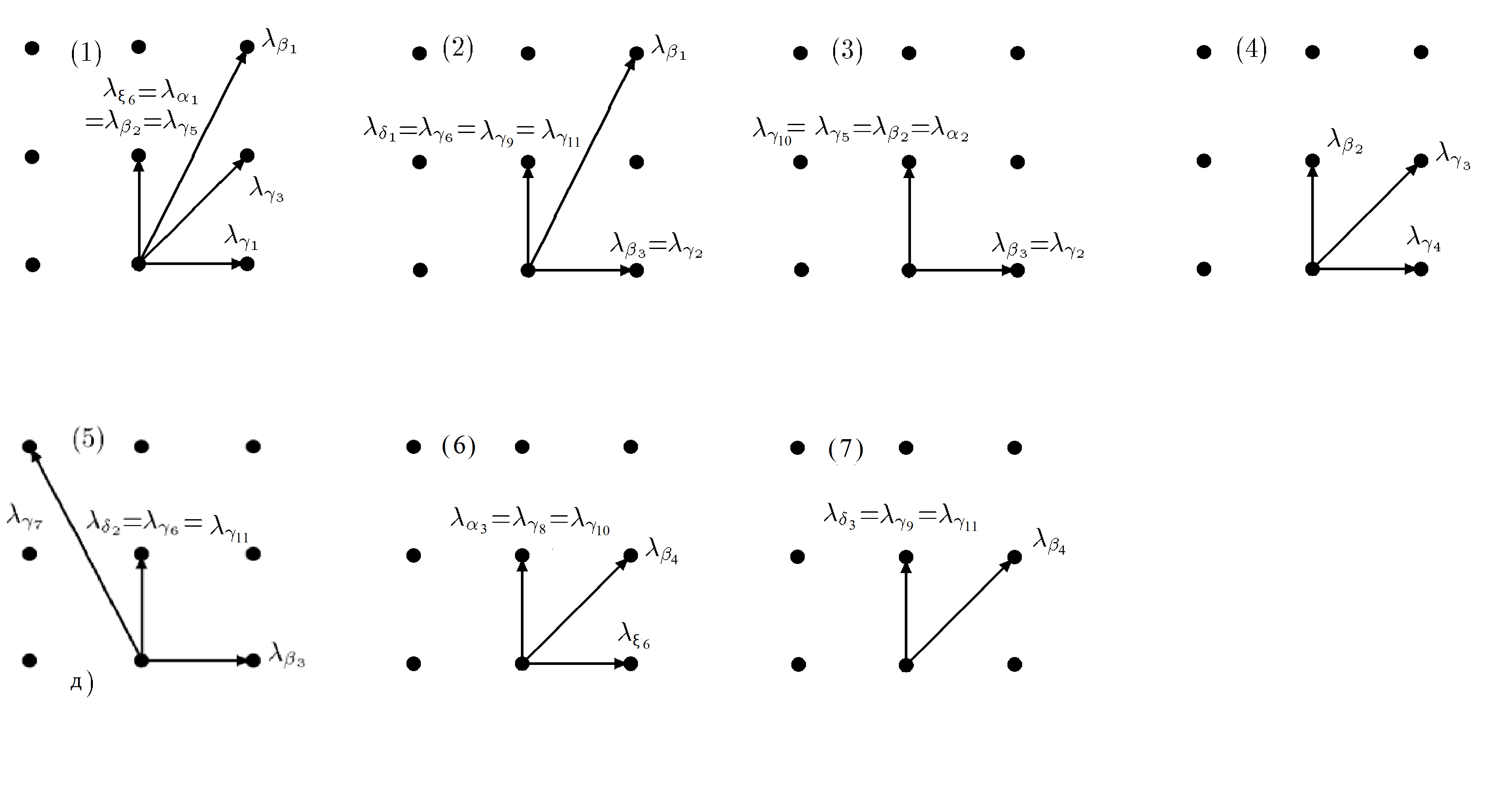
Remark 4.

The cycle $\lambda_{\beta_{4}}$ on tori of the family (6) (i.e. $\lambda_{\beta_{1}}$ on family I of tori in [14]) and $\lambda_{\beta_{4}}$ on tori of the family (7) (i.e. $\lambda_{\beta_{4}}$ on family V of tori in [14]) are expressed similarly by a choose of basis of the lattice.

Proof.

1. If an arc of $\Sigma$ and the type of bifurcation do not change when passing to a limiting case, then the corresponding admissible coordinate system also remains the same.

Therefore the admissible coordinate systems for the arcs $\alpha_{3},\beta_{4},\gamma_{10},\gamma_{11},\delta_{3},\xi_{6}$ are known from [14].

2. Singularities $w_{3}$ and $y_{12}$ are center-saddle $A\times B$ singularities, thus $\lambda_{\xi_{1}}=\pm\lambda_{\alpha_{1}}$ and $\lambda_{\gamma_{5}}=\pm\lambda_{\alpha_{1}}$ , i.e. $\lambda_{\xi_{1}}=\pm\lambda_{\gamma_{5}}$

The symmetry $(\alpha,x)\longrightarrow(-\alpha,-x)$ maps tori of families (2), (3), (5), (6) one to another and preserves $\mathrm{sgrad}\,H$ in the Sokolov case. It means that the direction of $\mathrm{sgrad}\,H$ coincides on two critical circles of the $C_{2}$ atom for the arcs $\gamma_{10},\gamma_{11}$ .

Thus $\lambda_{\xi_{1}}=\lambda_{\gamma_{5}}$ and $\lambda_{\xi_{2}}=\lambda_{\gamma_{6}}$ for the resulting foliations $B(\xi_{1})-B(\gamma_{5})$ and $B(\gamma_{6})-B(\xi_{2})$ after the perturbation of atoms $C_{2}(\xi_{3})$ and $2C_{2}(\xi_{4})$ .

3. Admissible coordinate systems for two arcs $\xi_{1},\xi_{2}$ can be calculated by considering a saddle-saddle singularity $w_{6}$ of the type $B\times B$ the same way as the singularity $U_{2}$ ( $y_{3}$ ) was studied in [2].

∎

Remark 5.

Using Theorem 3 we can calculate numerical marks $r,\varepsilon,n$ of the Fomenko–Zieschang invariants by well-known formulae, see [1]. (Molecules are directed by the acsending of the integral $K$ .)

We use notations from [6] for classes of regular foliations on isoenergy $Q^{3}$ .

Theorem 4.

1. For $b\neq 0$ all 25 classes of regular foliations on isoenergy $Q^{3}$ in the Kovalevskaya system on $\mathrm{so}(3,1)$ are non-equivalent, i.e. have different Fomenko–Zieschang invariants:

1.

10 classes $\mathbb{A}_{1},\mathbb{A}_{2},\mathbb{A}_{3},\mathbb{B}_{1},\mathbb{B}_{2},\mathbb{C}_{1},\mathbb{C}_{2},\mathbb{B}_{3},\mathbb{D}_{1},\mathbb{A}_{4}$ coincide with classes $A$ - $J$ respectively for the Kovalevskaya case on $\mathrm{e}(3)$ ,
2.

3 classes $\mathbb{E}_{1},\mathbb{E}_{2},\mathbb{F}_{1}$ coincide with classes $A,B,C$ of Sokolov case,
3.

6 classes $\mathbb{B}_{4},\mathbb{B}_{5},\mathbb{C}_{3},\mathbb{C}_{4},\mathbb{F}_{2},\mathbb{G}$ can be obtained from classes $E,F,I,H,D,G$ of Sokolov case by a typical perturbation $C_{2}\longrightarrow B\cfrac{r=\infty}{\varepsilon=1}B$ ,
4.

Fomenko-Zieschang invariants of classes $\mathbb{A}_{5},\mathbb{A}_{6},\mathbb{A}_{7},\mathbb{A}_{8},\mathbb{B}_{6},\mathbb{D}_{2}$ are shown in Fig. 5.

2. In the case of $b=0$ every foliation belongs to one of classes $A$ - $I$ of Sokolov case, $A$ - $D$ of Kovalevskaya case or $\mathbb{A}_{5},\mathbb{A}_{6}$ .

3. Foliations $\mathbb{A}_{5}$ and $\mathbb{A}_{5}$ belong to the classes $L_{26}$ and $L_{7}$ of Kovalevskaya integrable case on $\mathrm{so(4)}$ .

Remark 6.

Two foliations of the same Liouville class have the same structure of closures of almost all their trajectories.

5 Acknowledgements

This work was supported by the Russian Science Foundation (project no. 17-11-01303). Author is grateful to I. Kozlov for fruitful discussions and help.

References

[1] A. V. Bolsinov, A. T. Fomenko, Integrable Hamiltonian systems. Geometry, topology, classification, Udmurtian University Publishing House, Izhevsk, 1999.
[2] A. V. Bolsinov, P. H. Richter, A. T. Fomenko, The method of loop molecules and the topology of the Kovalevskaya top, Sbornik: Mathematics 191 2 (2000) 151–188.
[3] A. V. Borisov, I. S. Mamaev, V. V. Sokolov, A New Integrable Case on so(4), Doklady Physics 46 12 (2001) 888–889.
[4] M.P. Kharlamov, Bifurcation of common levels of first integrals of the Kovalevskaya problem, J. Appl. Math. and Mech. 47 (1983), 737–743.
[5] M. P. Kharlamov, Topological analysis of integrable problems of rigid body dynamics, Leningrad University Publishing House, Leningrad 1988, (Russian)
[6] M. P. Kharlamov, P. E. Ryabov, A. Yu. Savushkin, Topological Atlas of the Kowalevski-Sokolov Top, Regular and Chaotic Dynamics 21 1 (2016) 24–65.
[7] V. Kibkalo, Topological Analysis of the Liouville Foliation for the Kovalevskaya Integrable Case on the Lie Algebra so(4) Lobachevskii Journal of Mathematics, 39 9 (2018) 1396–1399.
[8] V. A. Kibkalo, Topological classification of Liouville foliations for the Kovalevskaya integrable case on the Lie algebra so(4), 2019, https://arxiv.org/abs/1901.09261 .
[9] I. V. Komarov, Kowalewski basis for the hydrogen atom, Theoret. and Math. Phys. 47 1 (1981) 320–324 [In Russian].
[10] I. V. Komarov, V. V. Sokolov, A. V. Tsiganov, Poisson Maps and Integrable Deformations of the Kowalevski Top, J. Phys. A, 36 29 (2003) 8035–8048.
[11] I. K. Kozlov, The topology of the Liouville foliation for the Kovalevskaya integrable case on the Lie algebra so(4), Sbornik: Mathematics, 205 4 (2014) 532–572.
[12] S. Kowalewski, Sur le probléme de la rotation d’un corps solide autour d’un point fixe, Acta Mathematica 12 (1889) 177–232.
[13] S. Kowalewski, Sur une propriété du systéme d’équations differentielles qui définit la rotation d’un corps solide autor d’un point fixe, Acta Mathematica 14 (1889) 81–93.
[14] P. V. Morozov, Topology of Liouville foliations in the Steklov and the Sokolov integrable cases of Kirchhoff’s equations, Sbornik: Mathematics 195 3 (2004) 369–412.
[15] A. A. Oshemkov, M. A. Tuzhilin, Integrable perturbations of saddle singularities of rank 0 of integrable Hamiltonian systems, Sbornik: Mathematics 209 9 (2018) 1351–1375.
[16] P. E. Ryabov, Bifurcations of first integrals in the Sokolov case, Theor. Math. Phys. 134 2 (2003) 181–197.
[17] V. V. Sokolov, A New Integrable Case for the Kirchhoff equation, Theor. Math. Phys. 129 1 (2001) 1335–1340.

Topological classification of Liouville foliations for the Kovalevskaya integrable case on the Lie algebra so(3, 1)Journal: Topology and its Applications

Abstract

Keywords:

2010 MSC

1 Introduction

2 Kovalevskaya case and its analogues

Theorem 1 ([10]).

Remark 1.

3 Bifurcation diagrams of the Kovalevskaya case on so⁡(3,1)\operatorname{so}(3,1)

3.1 Case of zero area integral (b=0b=0)

Theorem 2.

Remark 2.

Assertion 1.

Remark 3.

Proof.

Corollary 1.

3.2 Connections with the Kovalevskaya–Sokolov case

4 Liouville analysis of Kovalevskaya case on Lie algebra so⁡(3,1)\mathrm{so}(3,1)

Lemma 4.1.

Proof.

Theorem 3.

Remark 4.

Proof.

Remark 5.

Theorem 4.

Remark 6.

5 Acknowledgements

References

3 Bifurcation diagrams of the Kovalevskaya case on $\operatorname{so}(3,1)$

3.1 Case of zero area integral ( $b=0$ )

4 Liouville analysis of Kovalevskaya case on Lie algebra $\mathrm{so}(3,1)$