Compressed Distributed Gradient Descent: Communication-Efficient Consensus over NetworksThanks:  This work has been supported by NSF grants CNS-1527078, 1514260, 1446582, 1409336, 1012700, WiFiUS-1456806, ECCS-1444026, 1232118; ONR grant N00014-15-1-2166; ARO grant W911NF-14-1-0368; DTRA grants HDTRA 1-14-1-0058, 1-15-1-0003, AFRL VFRP’15 award; DARPA grant HROOll-15-C-0097and QNRF grant NPRP 7-923-2-344. DISTRIBUTION STATEMENT A: Approved for Public Release; distribution unlimited 88ABW-2015-5989 on Dec. 14, 2015.

In recent years, network consensus optimization has received increasing attention thanks to its generality and wide applicability. To date, network consensus optimization has found important applications in many scientific and engineering fields, e.g., distributed sensing in wireless sensor networks[1, 2, 3, 4], decentralized machine learning[5, 6], multi-agent robotic systems[7, 8, 9], smart grids[10, 11], to name just a few. Simply speaking, in a network consensus optimization problem, each node only has access to some component of the global objective function. That is, the global objective function is only partially known at each node. Through communications with local neighbors, all nodes in the network collaborate with each other and try to reach a consensus on an optimal solution, which minimizes the global objective function.

Among various algorithms for solving network consensus optimization problems, one of the most effective methods is the distributed gradient descent (DGD) algorithm, a first-order iterative method developed by Nedic and Ozdaglar approximately a decade ago[12]. The enduring popularity of DGD is primarily due to its implementation simplicity and elegant networking interpretation: In each iteration of DGD, each node performs an update by using a linear combination of a gradient step with respect to its local objective function and a weighted average from its local neighbors (also termed as a consensus step). It has been shown that DGD enjoys the same $O(1/k)$ convergence speed as the classical gradient descent method, where $k$ denotes the number of iterations[12]. The simplicity and salient features of DGD have further inspired a large number of extensions to various network settings (see Section II for more in-depth discussions).

However, despite its theoretical and engineering appeals, the performance of DGD may not always be satisfactory in practice. This is particularly true for solving a high-dimensional consensus problem over a network with low network communication speed. In this case, due to the large amount of data sharing and the communication bottleneck, exchanging full high-dimensional information between neighboring nodes is time-consuming (or even infeasible), which significantly hinders the overall convergence of DGD. To improve the convergence speed, several second-order approaches using Hessian approximation (with respect to local objective function) have been proposed (see, e.g., [13, 14]). Although these second-order methods converge in a fewer number of iterations (hence less information exchanges), they require matrix inversion in each iteration, implying a $\Omega(d^{2}\log d)$ per-iteration complexity for a $d$-dimensional problem. Hence, for high-dimensional consensus problems (i.e., large $d$), low-complexity first-order methods remain more preferable in practice.

To address DGD’s limitations in high-dimensional network consensus over low-speed networks, a naturally emerging idea is to compress the information exchanged between nodes. Specifically, by compressing the information in a high-dimensional state space to a smaller set of quantized states, each node can use a codebook to represent the quantized states with a small number of bits. Then, rather than directly transmitting full information, each node can just transmit the small-size codewords, which significantly reduces the communication burden. Moreover, from a cybersecurity standpoint, transmitting compressed information is also very helpful because each node can encrypt its codebook and avoid revealing full information to potential eavesdroppers in the network.

However, with compressed information being adopted in DGD, several fundamental questions immediately arise: i) Will DGD with compressed information exchanges still converge? ii) If the answer to i) is no, could we modify DGD to make it work with compressed information? iii) If the answer to ii) is yes, how fast does this modified DGD method converge? Indeed, answering all these questions are highly non-trivial and they constitute the main subjects of this paper. The main contribution in this paper is that we provide concrete answers to all three fundamental questions. Our key results and their significance are summarized as follows:

• •

  First, we show that DGD with straightforward compressed information exchange fails to converge because of a non-vanishing accumulated noise term resulted from compression over iterations. This motivates us to develop a noise variance reduction method. To this end, we propose a new idea called “amplified-differential compression DGD” (ADC-DGD), where, instead of directly exchanging compressed estimates of the global optimization variable in DGD, we exchange an amplified version of the state differential between consecutive iterations, hence the name. We show that ADC-DGD effectively diminishes the accumulated noise from compression and induces convergence.

• •

  We show that, under any unbiased compression operator, our ADC-DGD method converges at rate $O(1/k)$ to an $O(\alpha^{2})$-neighborhood of an optimal solution with a constant step-size $\alpha$. Under diminishing step-sizes, ADC-DGD converges asymptotically at rate $O(1/\sqrt{k})$ to an optimal solution. We note that these convergence rates are the best possible in the sense that they match with those of the original DGD without compression. This result is surprising since the information loss due to compression could be large. We also note that the convergence rate of ADC-DGD outperforms other existing distributed first-order methods with compression (see Section II for detailed discussions).

• •

  Based on the above convergence results of ADC-DGD, we further investigate the impacts of ADC-DGD’s amplifying factor on convergence speed and communication load. Interestingly, we reveal a phase transition phenomenon of the convergence speed with respect to the amplification exponent $\gamma$ in ADC-DGD. Specifically, when $\gamma\in(\frac{1}{2},1]$ (sublinear growth of amplification), convergence speed approaches that of DGD as $\gamma$ increases. However, as soon as $\gamma>1$, there is no further convergence speed improvement but network communication load continues to grow. This shows that $\gamma=1$ is a critical point, under which we can trade communication overhead for convergence speed.

Collectively, our results contribute to a growing theoretical foundation of network consensus optimization. The rest of the paper is organized as follows. In Section II, we review related work. In Section III, we introduce the network consensus optimization problem and show that DGD with compressed information exchange fails to converge. In Section IV, we present our ADC-DGD algorithm and its convergence performance analysis. Numerical results are provided in Section V and Section VI concludes this paper.

In this section, we first provide a quick overview on the historical development of DGD-type algorithms. We then focus on the recent advances of communication-conscious network consensus optimization, including related work that utilize compression.

1) DGD-Based Algorithms for Network Consensus: Network consensus optimization can trace its roots to the seminal work by Tsitsiklis [15], where the system model and the analysis framework were first developed. As mentioned earlier, a well-known method for solving network consensus optimization is the distributed (sub)gradient descent (DGD) method, which was proposed by Nedic and Ozdaglar in [12]. DGD was recently reexamined in [16] by Yuan et al. using a new Lyapunov technique, which offers further mathematical understanding of its convergence performance. In their follow-up work [17], the convergence behavior of DGD was further analyzed for non-convex problems. Recently, several DGD variants have been proposed to enhance the convergence performance (e.g., achieving the same $O(1/k)$ convergence rate with constant step-size [18] or even under time-varying network graphs [19]).

2) Communication-Conscious Distributed Optimization: As mentioned earlier, studies have shown that communication costs of DGD could be a major concern in practice. To this end, Chow et al. [20] studied the tradeoff between communication requirements and prescribed accuracy. In [21], Berahas et al. developed an adaptive DGD framework called $\text{DGD}^{t}$ to balance the costs between communication and computation. Here, the parameter $t$ represents the number of consensus steps performed per gradient descent step ($t=1$ corresponding to the original DGD). The larger the $t$-value, the cheaper the communication cost, and vice versa. The most related works to ours are by Reisizadeh et al.[22] and Tang et al.[23], which also consider adopting compression in DGD. The algorithm in [22], focusing on the strongly convex problems, used the diminishing step-size strategy to guarantee the convergence. In our work, we extend the strongly convexity assumption and prove the convengence both on diminishing step-size and constant step-size. However, our algorithm differs from [23] in the following key aspects: i) The compression in [23] uses a quantized extrapolation between two successive iterates, which can be viewed as a diminishing step-size strategy. In contrast, our ADC-DGD algorithm uses an amplified differential of two successive iterates. As will be shown later, our algorithm can be interpreted as a variance reduction method; ii) Our convergence rate outperforms that of [23]. The fastest convergence rate of the algorithms in [23] is $O(\log(k)/\sqrt{k})$, while the convergence rate of our ADC-DGD algorithm is $o(1/\sqrt{k})$; iii) To reach the best convergence rate in [23], the extrapolation compression algorithm needs to solve a complex equation to obtain an optimal step-size. In contrast, our ADC-DGD algorithm uses the standard sublinearly diminishing step-sizes, which is of much lower complexity and can be easily implemented in practice.

In Section III-A, we first introduce the network consensus optimization problem, which is followed by the basic version of the DGD method. Then in Section III-B, we will illustrate an example where DGD with directly compressed information fails to converge, which motivates our subsequent ADC-DGD approach in Section IV.

In this Section, we will first introduce our ADC-DGD algorithm in Section IV-A. Then, we will present the main theoretical results and their intuitions in Section IV-B. The proofs for the main results are provided in Section IV-C.

In this section, we will present several numerical experiments to further validate the performance of ADC-DGD.

1) Effect of Compression: First, we compare ADC-DGD with some existing methods to show its convergence rate and communication-efficiency. Consider a four-node network as shown in Fig. 4 with the following global objective function: $\min_{x}f(x)=f_{1}(x)+f_{2}(x)+f_{3}(x)+f_{4}(x)$, where $f_{1}(x)=-4x^{2}$, $f_{2}(x)=2(x-0.2)^{2}$, $f_{3}(x)=2(x+0.3)^{2}$, and $f_{4}(x)=5(x-0.1)^{2}$. It can be seen that $f_{1}(x)$ is non-convex, while the rest are convex. The communication consensus matrix used in this experiment is shown in Fig. 4.

In our simulation, we compare our ADC-DGD with the conventional DGD and $\text{DGD}^{t}.$ For $\text{DGD}^{t},$ we consider two cases: $t=3$ and $t=5.$ In ADC-DGD, the amplifying exponent $\gamma$ is set to $1$. We use two step-size strategies: 1) constant step-size $\alpha$ (i.e. $\eta=0$) and 2) diminishing step-size $\alpha/\sqrt{k}$ (i.e. $\eta=1/2$). We adopt the quantized operator in [25] as the compression operator. After compression, the values are integer. Hence, they can be stored as type ‘int16’, which is 2 bytes. However, the uncompressed values are stored as type ‘double’, costing 8 bytes. The convergence results for one trial are illustrated in Fig. 6 and Fig. 6.

From the simulations, we can see that: 1) with a fixed step-size, all algorithms converge to an error ball, while the radiuses of the conventional DGD and ADC-DGD are relatively smaller. This is because with a larger $t,$ $\beta^{t}$ becomes smaller and hence the error ball $O(\alpha/(1-\beta^{t}))$ for $\text{DGD}^{t}$ becomes larger; 2) By using compression, the convergence process of ADC-DGD is relatively less smooth. But the compression noise does not affect convergence. With the same step-size, the conventional DGD and ADC-DGD have the almost the same convergence rate; 3) By using diminishing step-sizes, the convergence speed for ADC-DGD becomes slower. However, the objective value remains decreasing; 4) By comparing the amount of exchanged information, ADC-DGD with the fixed step-size converges the fastest, using only 2000 bytes. This shows that our algorithm is the most communication-efficient.

2) Effect of the Amplifying Exponent: Next, we show the effect of the amplifying exponent $\gamma.$ As discussed in Section IV-D, with a small $\gamma,$ the noise caused by compression could lead to a slow convergence. On the other hand, with a large $\gamma,$ the transmitted value $k^{\gamma}y$ could be too large and cause overflow, especially for quantized compressed operator. Here, we change $\gamma$ using $\{0.6,0.8,1.0,1.2\}$ and keep the rest of the parameters the same. For each $\gamma,$ we repeat the algorithm $100$ times and compute the average objective values, as well as the maximum transmitted value from all the nodes in each iteration. The simulation results are shown in Figs. 8 and 8. We can see that, with a larger $\gamma$ value, the algorithm converges faster and the curve is smoother, while the transmitted values are increasing a little bit faster. In this example, we can see that $\gamma=0.8$ strikes a good balance between convergence and maximum transmitted value.

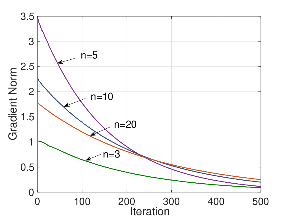
3) Effect of Network Size: The following simulations indicate that our algorithm could be scaled to large-size networks. In our simulation, we consider the ‘circle’ system: each node only connects with two neighboring nodes and forms a circle. For example, Fig. 10 shows a five-node circle. We set $n$ to be $3$, $5$, $10$, $20$ in our experiment. The local objectives are in the form of $f_{i}(x)=a_{i}(x-b_{i})^{2}.$ In our simulation, $\{a_{i},b_{i}\}_{i=1}^{n}$ are independently randomly generated: $a_{i}\sim\text{Uniform}[0,10]$ and $b_{i}\sim\text{Uniform}[0,1]$. For each value of $n$, we repeat $100$ trials and compute the average gradient norm. The convergence results are shown in Fig. 10. It can be seen that our algorithm works well as the network size increases, demonstrating the scalability of ADC-DGD.

In this paper, we considered designing communication-efficient network consensus optimization algorithms in networks with slow communication rates. We proposed a new algorithm called amplified-differential compression decentralized gradient descent (ADC-DGD), which is based on compression to reduce communication costs. We investigated the convergence behavior of ADC-DGD on smooth but possibly non-convex objectives in this work. We showed that: 1) by employing a fixed step-size $\alpha$, ADC-DGD converges with the $O(1/k^{\min(1,\gamma)})$ ergodic rate until reaching an error ball of size $O(\alpha^{2})$ with the amplified parameter $\gamma$; 2) ADC-DGD enjoys the best convergence rate $o(1/\sqrt{k})$ and converge to a stationary point almost surely with diminishing step-sizes. Consensus optimization with compressed information is an important and under-explored area. An interesting future topic is to generalize our ADC-DGD algorithmic framework to analyze cases with local stochastic gradients, which could further lower the implementation complexity of ADC-DGD.

References

• [1] Q. Ling and Z. Tian, “Decentralized sparse signal recovery for compressive sleeping wireless sensor networks,” IEEE Transactions on Signal Processing, vol. 58, no. 7, pp. 3816–3827, 2010.
• [2] J. B. Predd, S. R. Kulkarni, and H. V. Poor, “Distributed learning in wireless sensor networks,” arXiv preprint cs/0503072, 2005.
• [3] I. D. Schizas, A. Ribeiro, and G. B. Giannakis, “Consensus in ad hoc wsns with noisy links—part i: Distributed estimation of deterministic signals,” IEEE Transactions on Signal Processing, vol. 56, no. 1, pp. 350–364, 2008.
• [4] F. Zhao, J. Shin, and J. Reich, “Information-driven dynamic sensor collaboration,” IEEE Signal processing magazine, vol. 19, no. 2, pp. 61–72, 2002.
• [5] J. C. Duchi, A. Agarwal, and M. J. Wainwright, “Dual averaging for distributed optimization: Convergence analysis and network scaling,” IEEE Transactions on Automatic control, vol. 57, no. 3, pp. 592–606, 2012.
• [6] K. I. Tsianos, S. Lawlor, and M. G. Rabbat, “Consensus-based distributed optimization: Practical issues and applications in large-scale machine learning,” in Communication, Control, and Computing (Allerton), 2012 50th Annual Allerton Conference on. IEEE, 2012, pp. 1543–1550.
• [7] Y. Cao, W. Yu, W. Ren, and G. Chen, “An overview of recent progress in the study of distributed multi-agent coordination,” IEEE Transactions on Industrial informatics, vol. 9, no. 1, pp. 427–438, 2013.
• [8] W. Ren, R. W. Beard, and E. M. Atkins, “Information consensus in multivehicle cooperative control,” IEEE Control Systems, vol. 27, no. 2, pp. 71–82, 2007.
• [9] K. Zhou, S. I. Roumeliotis et al., “Multirobot active target tracking with combinations of relative observations,” IEEE Transactions on Robotics, vol. 27, no. 4, pp. 678–695, 2011.
• [10] G. B. Giannakis, V. Kekatos, N. Gatsis, S.-J. Kim, H. Zhu, and B. F. Wollenberg, “Monitoring and optimization for power grids: A signal processing perspective,” IEEE Signal Processing Magazine, vol. 30, no. 5, pp. 107–128, 2013.
• [11] V. Kekatos and G. B. Giannakis, “Distributed robust power system state estimation,” IEEE Transactions on Power Systems, vol. 28, no. 2, pp. 1617–1626, 2013.
• [12] A. Nedic and A. Ozdaglar, “Distributed subgradient methods for multi-agent optimization,” IEEE Transactions on Automatic Control, vol. 54, no. 1, pp. 48–61, 2009.
• [13] M. I. Jordan, J. D. Lee, and Y. Yang, “Communication-efficient distributed statistical inference,” arXiv preprint arXiv:1605.07689, 2016.
• [14] J. Wang, M. Kolar, N. Srebro, and T. Zhang, “Efficient distributed learning with sparsity,” arXiv preprint arXiv:1605.07991, 2016.
• [15] J. N. Tsitsiklis, “Problems in decentralized decision making and computation.” MASSACHUSETTS INST OF TECH CAMBRIDGE LAB FOR INFORMATION AND DECISION SYSTEMS, Tech. Rep., 1984.
• [16] K. Yuan, Q. Ling, and W. Yin, “On the convergence of decentralized gradient descent,” SIAM Journal on Optimization, vol. 26, no. 3, pp. 1835–1854, 2016.
• [17] J. Zeng and W. Yin, “On nonconvex decentralized gradient descent,” arXiv preprint arXiv:1608.05766, 2016.
• [18] W. Shi, Q. Ling, G. Wu, and W. Yin, “Extra: An exact first-order algorithm for decentralized consensus optimization,” SIAM Journal on Optimization, vol. 25, no. 2, pp. 944–966, 2015.
• [19] A. Nedic, A. Olshevsky, and W. Shi, “Achieving geometric convergence for distributed optimization over time-varying graphs,” SIAM Journal on Optimization, vol. 27, no. 4, pp. 2597–2633, 2017.
• [20] Y.-T. Chow, W. Shi, T. Wu, and W. Yin, “Expander graph and communication-efficient decentralized optimization,” in Signals, Systems and Computers, 2016 50th Asilomar Conference on. IEEE, 2016, pp. 1715–1720.
• [21] A. S. Berahas, R. Bollapragada, N. S. Keskar, and E. Wei, “Balancing communication and computation in distributed optimization,” arXiv preprint arXiv:1709.02999, 2017.
• [22] A. Reisizadeh, A. Mokhtari, H. Hassani, and R. Pedarsani, “Quantized decentralized consensus optimization,” in 2018 IEEE Conference on Decision and Control (CDC). IEEE, 2018, pp. 5838–5843.
• [23] H. Tang, C. Zhang, S. Gan, T. Zhang, and J. Liu, “Decentralization meets quantization,” arXiv preprint arXiv:1803.06443, 2018.
• [24] Y. Zhang, M. J. Wainwright, and J. C. Duchi, “Communication-efficient algorithms for statistical optimization,” in Advances in Neural Information Processing Systems, 2012, pp. 1502–1510.
• [25] D. Alistarh, D. Grubic, J. Li, R. Tomioka, and M. Vojnovic, “Qsgd: Communication-efficient sgd via gradient quantization and encoding,” in Advances in Neural Information Processing Systems, 2017, pp. 1707–1718.
• [26] W. Wen, C. Xu, F. Yan, C. Wu, Y. Wang, Y. Chen, and H. Li, “Terngrad: Ternary gradients to reduce communication in distributed deep learning,” in Advances in Neural Information Processing Systems, 2017, pp. 1508–1518.
• [27] J. Wangni, J. Wang, J. Liu, and T. Zhang, “Gradient sparsification for communication-efficient distributed optimization,” arXiv preprint arXiv:1710.09854, 2017.
• [28] X. Zhang, J. Liu, and Z. Zhu, “Taming convergence for asynchronous stochastic gradient descent with unbounded delay in non-convex learning,” arXiv preprint arXiv:1805.09470, 2018.
• [29] R. Hannah and W. Yin, “On unbounded delays in asynchronous parallel fixed-point algorithms,” Journal of Scientific Computing, pp. 1–28, 2016.
Appendix A Proof for Lemma 1
Without loss of generality, we prove the case of one-dimensional objective. Firstly, we consider fi​(⋅)f_{i}(\cdot) reach the minimal at xi∗=0x_{i}^{*}=0 and fi​(xi∗)=0.f_{i}(x_{i}^{*})=0. With the convexity of fi​(⋅),f_{i}(\cdot), fi​(x)≤(1−1a)​fi​(0)+1a​fi​(a​x),f_{i}(x)\leq(1-\frac{1}{a})f_{i}(0)+\frac{1}{a}f_{i}(ax), ∀x,a>1.\forall x,~a>1. Consider x0x_{0} with fi​(x0)≠0,f_{i}(x_{0})\neq 0, and define maxi⁡{‖x0‖fi​(x0)}=M0.\max_{i}\{\frac{\|x_{0}\|}{f_{i}(x_{0})}\}=M_{0}. Consider ∀y>x0>0,\forall y>x_{0}>0, there exists a constant ay>1a_{y}>1 such that y=ay​x0y=a_{y}x_{0} and thus fi​(x0)≤1ay​fi​(y).f_{i}(x_{0})\leq\frac{1}{a_{y}}f_{i}(y). Hence, ‖y‖fi​(y)≤‖ay​x0‖ay​fi​(x0)≤M0.\frac{\|y\|}{f_{i}(y)}\leq\frac{\|a_{y}x_{0}\|}{a_{y}f_{i}(x_{0})}\leq M_{0}. It is easy to obtain the same result for negative values y.y. Therefore, ∑i=1N‖xi‖∑i=1Nfi​(xi)≤∑i=1N‖xi‖fi​(xi)≤N​M0:=M.\frac{\sum_{i=1}^{N}\|x_{i}\|}{\sum_{i=1}^{N}f_{i}(x_{i})}\leq\sum_{i=1}^{N}\frac{\|x_{i}\|}{f_{i}(x_{i})}\leq NM_{0}:=M. Next, if xi∗≠0x_{i}^{*}\neq 0 and fi​(xi∗)≠0.f_{i}(x_{i}^{*})\neq 0. Consider the transformation, gi​(x)=fi​(x+xi∗)−fi​(xi∗),g_{i}(x)=f_{i}(x+x_{i}^{*})-f_{i}(x_{i}^{*}), then x=0x=0 is the minimal solution for gi​(x),g_{i}(x), gi​(0)=0g_{i}(0)=0 and also gi​(x)g_{i}(x) maintains the convexity. From the above, we know that ‖x‖gi​(x)≤M0.\frac{\|x\|}{g_{i}(x)}\leq M_{0}. Therefore, ‖x‖fi​(x+xi∗)−fi​(xi∗)≤M0.\frac{\|x\|}{f_{i}(x+x_{i}^{*})-f_{i}(x_{i}^{*})}\leq M_{0}. Denote y=x+xi∗,y=x+x_{i}^{*}, we have ‖y−xi∗‖fi​(y)−fi​(xi∗)≤M0.\frac{\|y-x_{i}^{*}\|}{f_{i}(y)-f_{i}(x_{i}^{*})}\leq M_{0}. Consider the following limits:
lim‖y‖→∞‖y‖fi​(y)/‖y−xi∗‖f⁡(y)−fi​(xi∗)=lim‖y‖→∞‖y‖‖y−xi∗‖/fi​(y)fi​(y)−fi​(xi∗)\displaystyle\lim_{\|y\|\rightarrow\infty}\!\!\frac{\|y\|}{f_{i}(y)}\!/\!\frac{\|y-x_{i}^{*}\|}{f(y)-f_{i}(x_{i}^{*})}\!\!=\!\!\lim_{\|y\|\rightarrow\infty}\!\!\frac{\|y\|}{\|y-x_{i}^{*}\|}\!/\!\frac{f_{i}(y)}{f_{i}(y)-f_{i}(x_{i}^{*})}
=lim‖y‖→∞fi​(y)−fi​(xi∗)fi​(y)≤1+lim‖y‖→∞|fi​(xi∗)fi​(y)|≤2,\displaystyle=\lim_{\|y\|\rightarrow\infty}\frac{f_{i}(y)-f_{i}(x_{i}^{*})}{f_{i}(y)}\leq 1+\lim_{\|y\|\rightarrow\infty}|\frac{f_{i}(x_{i}^{*})}{f_{i}(y)}|\leq 2,
which implies that lim‖y‖→∞‖y‖fi​(y)≤2​M0.\lim_{\|y\|\rightarrow\infty}\frac{\|y\|}{f_{i}(y)}\leq 2M_{0}. Similarly, we can show ∑i=1N‖xi‖∑i=1Nfi​(xi)≤2​N​M0:=M.\frac{\sum_{i=1}^{N}\|x_{i}\|}{\sum_{i=1}^{N}f_{i}(x_{i})}\leq 2NM_{0}:=M. This completes the proof.
Appendix B Proof for Theorem 4
First, we give the following useful lemma for series with converged infinite sum.
Lemma 5.
Assume the infinite sum of the positive series {ak}k=1∞,\{a_{k}\}_{k=1}^{\infty}, ∑k=1∞ak<∞,\sum_{k=1}^{\infty}a_{k}<\infty, then ak=o⁡(1/k).a_{k}=o(1/k).
Proof.
This result has been discussed in [28]. We give the details in the following. Define {bk}k=1∞\{b_{k}\}_{k=1}^{\infty} with bk=1/k.b_{k}=1/k. With the properity of pp-series, it is well-known that ∑k=1∞bk=∞.\sum_{k=1}^{\infty}b_{k}=\infty.
Now, if we assume aka_{k} is higher order than o⁡(1/k),o(1/k), then limk→∞ak/bk=c,\lim_{k\rightarrow\infty}a_{k}/b_{k}=c, where c=(0,+∞)∪{+∞}.c=(0,+\infty)\cup\{+\infty\}. With the limit comparison test, then ∑k=1∞ak<∞,\sum_{k=1}^{\infty}a_{k}<\infty, which leads to a contradiction with the fact ∑k=1∞ak<∞.\sum_{k=1}^{\infty}a_{k}<\infty. Hence, it requires that c=0c=0 and ak=o⁡(1/k).a_{k}=o(1/k). ∎
Define the filtrations {ℱk=σ⟨x1,⋯,xk⟩}\{\mathcal{F}_{k}=\sigma\langle\textbf{x}^{1},\cdots,\textbf{x}^{k}\rangle\}, ℱk⊂ℱk+1.\mathcal{F}_{k}\subset\mathcal{F}_{k+1}. From Lemma 2, given α,\alpha, the Lyapunov function Lα​(x)L_{\alpha}(\textbf{x}) has (1−λn​(W)+α​L)(1-\lambda_{n}(\textbf{W})+\alpha L)-Lipschitz gradient. Hence, the following holds:
Lα​(xk+1)\displaystyle L_{\alpha}(\textbf{x}^{k+1}) ≤(a)Lα​(xk)+⟨∇Lα​(xk),xk+1−xk⟩\displaystyle\stackrel{{\scriptstyle(a)}}{{\leq}}L_{\alpha}(\textbf{x}^{k})+\langle\nabla L_{\alpha}(\textbf{x}^{k}),\textbf{x}^{k+1}-\textbf{x}^{k}\rangle
+12​(1−λn​(W)+α​L)​‖xk+1−xk‖2\displaystyle+\frac{1}{2}(1-\lambda_{n}(\textbf{W})+\alpha L)\|\textbf{x}^{k+1}-\textbf{x}^{k}\|^{2}
=(b)Lα​(xk)−⟨∇Lα​(xk),∇Lα​(xk)−W​ϵkkγ⟩\displaystyle\stackrel{{\scriptstyle(b)}}{{=}}L_{\alpha}(\textbf{x}^{k})-\langle\nabla L_{\alpha}(\textbf{x}^{k}),\nabla L_{\alpha}(\textbf{x}^{k})-\frac{\textbf{W}\epsilon^{k}}{k^{\gamma}}\rangle
+(1−λn​(W)+α​L)2​‖∇Lα​(xk)−W​ϵkkγ‖2\displaystyle+\frac{(1-\lambda_{n}(\textbf{W})+\alpha L)}{2}\|\nabla L_{\alpha}(\textbf{x}^{k})-\frac{\textbf{W}\epsilon^{k}}{k^{\gamma}}\|^{2}
=Lα​(xk)−‖∇Lα​(xk)‖2+⟨∇Lα​(xk),W​ϵkkγ⟩\displaystyle=L_{\alpha}(\textbf{x}^{k})-\|\nabla L_{\alpha}(\textbf{x}^{k})\|^{2}+\langle\nabla L_{\alpha}(\textbf{x}^{k}),\frac{\textbf{W}\epsilon^{k}}{k^{\gamma}}\rangle
+(1−λn​(W)+α​L)2[∥∇Lα(xk)∥2\displaystyle+\frac{(1-\lambda_{n}(\textbf{W})+\alpha L)}{2}[\|\nabla L_{\alpha}(\textbf{x}^{k})\|^{2}
+∥W​ϵkkγ∥2−2⟨∇Lα(xk),W​ϵkkγ⟩],\displaystyle+\|\frac{\textbf{W}\epsilon^{k}}{k^{\gamma}}\|^{2}-2\langle\nabla L_{\alpha}(\textbf{x}^{k}),\frac{\textbf{W}\epsilon^{k}}{k^{\gamma}}\rangle],
where (a) is from (1−λn​(W)+α​L)(1-\lambda_{n}(\textbf{W})+\alpha L)-Lipschitz condition for Lα​(x)L_{\alpha}(\textbf{x}); (b) is from Equation IV-C. Take the condtional expectation on the above inequality:
𝔼\displaystyle\mathbb{E} [Lα​(xk+1)|ℱk]\displaystyle[L_{\alpha}(\textbf{x}^{k+1})|\mathcal{F}_{k}]
≤Lα​(xk)−‖∇Lα​(xk)‖2\displaystyle\leq L_{\alpha}(\textbf{x}^{k})-\|\nabla L_{\alpha}(\textbf{x}^{k})\|^{2}
+(1−λn​(W)+α​L)2​[‖∇Lα​(xk)‖2+𝔼⁡[‖W​ϵkkγ‖2]]\displaystyle+\frac{(1-\lambda_{n}(\textbf{W})+\alpha L)}{2}[\|\nabla L_{\alpha}(\textbf{x}^{k})\|^{2}+\mathbb{E}[\|\frac{\textbf{W}\epsilon^{k}}{k^{\gamma}}\|^{2}]]
≤(c)Lα​(xk)−‖∇Lα​(xk)‖2\displaystyle\stackrel{{\scriptstyle(c)}}{{\leq}}L_{\alpha}(\textbf{x}^{k})-\|\nabla L_{\alpha}(\textbf{x}^{k})\|^{2}
+(1−λn​(W)+α​L)2​[‖∇Lα​(xk)‖2+n​σ2k2​γ]\displaystyle+\frac{(1-\lambda_{n}(\textbf{W})+\alpha L)}{2}[\|\nabla L_{\alpha}(\textbf{x}^{k})\|^{2}+\frac{n\sigma^{2}}{k^{2\gamma}}]
=Lα​(xk)−(1−(1−λn​(W)+α​L)2)​‖∇Lα​(xk)‖2\displaystyle=L_{\alpha}(\textbf{x}^{k})-(1-\frac{(1-\lambda_{n}(\textbf{W})+\alpha L)}{2})\|\nabla L_{\alpha}(\textbf{x}^{k})\|^{2}
+(1−λn​(W)+α​L)​n​σ22​k2​γ,\displaystyle+\frac{(1-\lambda_{n}(\textbf{W})+\alpha L)n\sigma^{2}}{2k^{2\gamma}},
where (c) is from the inequality 12. Thus, with α<1+λn​(W)L\alpha<\frac{1+\lambda_{n}(\textbf{W})}{L} and take the full expectation:
𝔼⁡[Lα​(xk+1)]+(1+λn​(W)−α​L)2​𝔼​[‖∇Lα​(xk)‖2]\displaystyle\mathbb{E}[L_{\alpha}(\textbf{x}^{k+1})]+\frac{(1+\lambda_{n}(\textbf{W})-\alpha L)}{2}\mathbb{E}[\|\nabla L_{\alpha}(\textbf{x}^{k})\|^{2}]
≤𝔼⁡[Lα​(xk)]+(1−λn​(W)+α​L)​n​σ22​k2​γ,\displaystyle\leq\mathbb{E}[L_{\alpha}(\textbf{x}^{k})]+\frac{(1-\lambda_{n}(\textbf{W})+\alpha L)n\sigma^{2}}{2k^{2\gamma}},
where (1+λn​(W)−α​L)2>0.\frac{(1+\lambda_{n}(\textbf{W})-\alpha L)}{2}>0. Telescoping the above inequality, we have:
𝔼⁡[Lα​(xk+1)]+∑i=0k(1+λn​(W)−α​L)2​𝔼​[‖∇Lα​(xi)‖2]\displaystyle\mathbb{E}[L_{\alpha}(\textbf{x}^{k+1})]+\sum_{i=0}^{k}\frac{(1+\lambda_{n}(\textbf{W})-\alpha L)}{2}\mathbb{E}[\|\nabla L_{\alpha}(\textbf{x}^{i})\|^{2}]
≤Lα​(x0)+∑i=0k(1−λn​(W)+α​L)​n​σ22​i2​γ,\displaystyle\leq L_{\alpha}(\textbf{x}^{0})+\sum_{i=0}^{k}\frac{(1-\lambda_{n}(\textbf{W})+\alpha L)n\sigma^{2}}{2i^{2\gamma}}, (15)
which implies that
∑i=0k(1+λn​(W)−α​L)2​𝔼​[‖∇Lα​(xi)‖2]\displaystyle\sum_{i=0}^{k}\frac{(1+\lambda_{n}(\textbf{W})-\alpha L)}{2}\mathbb{E}[\|\nabla L_{\alpha}(\textbf{x}^{i})\|^{2}] (16)
≤Lα​(x0)−𝔼⁡[Lα​(xk+1)]+∑i=0k(1−λn​(W)+α​L)​n​σ22​i2​γ\displaystyle\leq L_{\alpha}(\textbf{x}^{0})-\mathbb{E}[L_{\alpha}(\textbf{x}^{k+1})]+\sum_{i=0}^{k}\frac{(1-\lambda_{n}(\textbf{W})+\alpha L)n\sigma^{2}}{2i^{2\gamma}}
≤(d)Lα​(x0)−α​∑i=1nfi​(x∗)+∑i=0k(1−λn​(W)+α​L)​n​σ22​i2​γ\displaystyle\stackrel{{\scriptstyle(d)}}{{\leq}}L_{\alpha}(\textbf{x}^{0})-\alpha\sum_{i=1}^{n}f_{i}(x^{*})+\sum_{i=0}^{k}\frac{(1-\lambda_{n}(\textbf{W})+\alpha L)n\sigma^{2}}{2i^{2\gamma}} (17)
where (d) is because 1) the eigenvalues of (I−W)(\textbf{I}-\textbf{W}) are positive and 12​xT​(I−W)​x≥0\frac{1}{2}\textbf{x}^{T}(\textbf{I}-\textbf{W})\textbf{x}\geq 0 and 2) ∑i=1nfi​(x∗)≤∑i=1nfi​(x),\sum_{i=1}^{n}f_{i}(x^{*})\leq\sum_{i=1}^{n}f_{i}(x), ∀x,\forall x, thus,
Lα​(xk+1)=12​(xk+1)T​(I−W)​xk+1+α​∑i=1nfi​(xi,k+1)≥α​∑i=1nfi​(x∗).L_{\alpha}(\textbf{x}^{k+1})=\frac{1}{2}(\textbf{x}^{k+1})^{T}(\textbf{I}-\textbf{W})\textbf{x}^{k+1}+\alpha\sum_{i=1}^{n}f_{i}(x_{i,k+1})\geq\alpha\sum_{i=1}^{n}f_{i}(x^{*}).
With the condition γ>12,\gamma>\frac{1}{2}, Equation (16) indicates that ∑i=0∞𝔼⁡[‖∇Lα​(xi)‖2]\sum_{i=0}^{\infty}\mathbb{E}[\|\nabla L_{\alpha}(\textbf{x}^{i})\|^{2}] is bounded and 𝔼⁡[‖∇Lα​(xi)‖2]=o⁡(1/k),\mathbb{E}[\|\nabla L_{\alpha}(\textbf{x}^{i})\|^{2}]=o(1/k), due to Lemma 5. Also, from Equation B, 𝔼⁡[Lα​(xk)]<+∞\mathbb{E}[L_{\alpha}(\textbf{x}^{k})]<+\infty holds, ∀k\forall k.
Due to the fact that
𝔼⁡[∑i=1nfi​(xi,k)]≤𝔼⁡[1α​Lα​(xk)]<+∞,\mathbb{E}[\sum_{i=1}^{n}f_{i}(x_{i,k})]\leq\mathbb{E}[\frac{1}{\alpha}L_{\alpha}(\textbf{x}^{k})]<+\infty,
with Assumption 2, the following holds:
𝔼[∥xk\displaystyle\mathbb{E}[\|\textbf{x}^{k} ∥]≤∫‖xk‖≤A∥xk∥p(xk)d(xk)+∫‖xk‖>A∥xk∥p(xk)d(xk)\displaystyle\|]\leq\int_{\|\textbf{x}^{k}\|\leq A}\|\textbf{x}^{k}\|p(\textbf{x}^{k})d(\textbf{x}^{k})+\int_{\|\textbf{x}^{k}\|>A}\|\textbf{x}^{k}\|p(\textbf{x}^{k})d(\textbf{x}^{k})
≤∫‖xk‖≤AA​p​(xk)​d​(xk)+∫‖xk‖>A‖xk‖f⁡(xk)​f​(xk)​p​(xk)​d​(xk)\displaystyle\leq\int_{\|\textbf{x}^{k}\|\leq A}Ap(\textbf{x}^{k})d(\textbf{x}^{k})+\int_{\|\textbf{x}^{k}\|>A}\frac{\|\textbf{x}^{k}\|}{f(\textbf{x}^{k})}f(\textbf{x}^{k})p(\textbf{x}^{k})d(\textbf{x}^{k})
≤A+(M+δA)​𝔼​[f⁡(xk)]≤+∞\displaystyle\leq A+(M+\delta_{A})\mathbb{E}[f(\textbf{x}^{k})]\leq+\infty
where p⁡(xk)p(\textbf{x}^{k}) is the density of xk\textbf{x}^{k} and δA\delta_{A} is from the fact that ∀A>0\forall A>0, there exist δA<∞,\delta_{A}<\infty, such that |‖xk‖f⁡(xk)|<M+δA.|\frac{\|\textbf{x}^{k}\|}{f(\textbf{x}^{k})}|<M+\delta_{A}. Hence 𝔼⁡[‖xk‖]\mathbb{E}[\|\textbf{x}^{k}\|] is bounded, ∀k,\forall k, say bounded by B.B. Then,
𝔼​[‖∇f​(xk)‖]\displaystyle\mathbb{E}[\|\nabla f(\textbf{x}^{k})\|] =𝔼⁡[‖∇f​(xk)−∇f​(x∗)‖]\displaystyle=\mathbb{E}[\|\nabla f(\textbf{x}^{k})-\nabla f(\textbf{x}^{*})\|]
≤L​𝔼​[‖xk−x∗‖]≤L⁡(B+‖x∗‖).\displaystyle\leq L\mathbb{E}[\|\textbf{x}^{k}-\textbf{x}^{*}\|]\leq L(B+\|\textbf{x}^{*}\|).
∎
Appendix C Proof for Lemma3
First of all, hkh_{k} could be bounded by a integral hk=βk​∑i=1kβ−iiγ≤βk​(∫x=1kβ−xx​𝑑x+k)h_{k}=\beta^{k}\sum_{i=1}^{k}\frac{\beta^{-i}}{i^{\gamma}}\leq\beta^{k}(\int_{x=1}^{k}\frac{\beta^{-x}}{x}dx+k). Thus, we focus on the increasing rate of ∫x=1kβ−xx​𝑑x.\int_{x=1}^{k}\frac{\beta^{-x}}{x}dx. Denote z:=−log⁡(β)>0z:=-\log(\beta)>0 and s:=1−γ∈(0,1),s:=1-\gamma\in(0,1), we have the following complex integral:
∫x=1kβ−xxγ=∫x=1kez​xx1−s​𝑑x=(a)∫y=zz​key(y/z)1−s​z​𝑑y\displaystyle\int_{x=1}^{k}\frac{\beta^{-x}}{x^{\gamma}}\!=\!\int_{x=1}^{k}\frac{e^{zx}}{x^{1-s}}dx\!\stackrel{{\scriptstyle(a)}}{{=}}\!\int_{y=z}^{zk}\frac{e^{y}}{(y/z)^{1-s}z}dy
=z−s​∫y=zz​keyy1−s​𝑑y=(b)z−s​∫t=e−i​π​ze−i​π​z​ke−t​ts−1​ei​π​s​𝑑t\displaystyle\!=\!z^{-s}\!\!\int_{y=z}^{zk}\frac{e^{y}}{y^{1-s}}dy\stackrel{{\scriptstyle(b)}}{{=}}z^{-s}\int_{t=e^{-i\pi}z}^{e^{-i\pi}zk}e^{-t}t^{s-1}e^{i\pi s}dt
=z−s​ei​π​s​[∫t=e−i​π​z∞e−t​ts−1​𝑑t−∫t=e−i​π​k​z∞e−t​ts−1​𝑑t]\displaystyle=z^{-s}e^{i\pi s}[\int_{t=e^{-i\pi}z}^{\infty}e^{-t}t^{s-1}dt-\int_{t=e^{-i\pi}kz}^{\infty}e^{-t}t^{s-1}dt]
=(c)z−s​ei​π​s​[Γ⁡(s,e−i​π​z)−Γ⁡(s,e−i​π​k​z)],\displaystyle\stackrel{{\scriptstyle(c)}}{{=}}z^{-s}e^{i\pi s}[\Gamma(s,e^{-i\pi}z)-\Gamma(s,e^{-i\pi}kz)],
where y=z​xy=zx in (a), t=e−i​π​yt=e^{-i\pi}y in (b) with e−i​π+1=0e^{-i\pi}+1=0 and Γ⁡(⋅,⋅)\Gamma(\cdot,\cdot) is the upper incomplete gamma function in (c). With the properity of Γ⁡(⋅,⋅),\Gamma(\cdot,\cdot), it follows that as k→+∞,k\rightarrow+\infty, Γ⁡(s,e−i​π​k​z)=(e−i​π​k​z)s−1​ek​z​[1+O⁡(1k)]\Gamma(s,e^{-i\pi}kz)=(e^{-i\pi}kz)^{s-1}e^{kz}[1+O(\frac{1}{k})], which implies the second term on the above equation is z−s​ei​π​s​Γ​(s,e−i​π​k​z)=−z−1​k−γ​β−k​[1+O⁡(1k)]z^{-s}e^{i\pi s}\Gamma(s,e^{-i\pi}kz)=-z^{-1}k^{-\gamma}\beta^{-k}[1+O(\frac{1}{k})]. Hence, the integral is ∫x=1kβk−xxγ=βk​{z−s​ei​π​s​Γ​(s,e−i​π​z)+z−1​k−γ​β−k​[1+O⁡(1k)]}=1k−γ​z​[1+O⁡(1k)]+O⁡(βk)\int_{x=1}^{k}\frac{\beta^{k-x}}{x^{\gamma}}=\beta^{k}\{z^{-s}e^{i\pi s}\Gamma(s,e^{-i\pi}z)+z^{-1}k^{-\gamma}\beta^{-k}[1+O(\frac{1}{k})]\}=\frac{1}{k^{-\gamma}z}[1+O(\frac{1}{k})]+O(\beta^{k}), and hk=O⁡(1kγ).h_{k}=O(\frac{1}{k^{\gamma}}). This completes the proof.
Appendix D Proof for Theorem 1
It is knowns that that x¯k=1n​11T​xk.\bar{\textbf{x}}^{k}=\frac{1}{n}\textbf{11}^{T}\textbf{x}^{k}. As a result,
‖xk−x¯k‖=‖xk−1n​11T​xk‖\displaystyle\|\textbf{x}^{k}-\bar{\textbf{x}}^{k}\|=\|\textbf{x}^{k}-\frac{1}{n}\textbf{11}^{T}\textbf{x}^{k}\|
=(a)∥(I−1n11T)∑i=0k−1[−αiWk−i−1∇f(xi)+Wk−iϵiiγ]∥\displaystyle\stackrel{{\scriptstyle(a)}}{{=}}\|(\textbf{I}-\frac{1}{n}\textbf{11}^{T})\sum_{i=0}^{k-1}[-\alpha_{i}\textbf{W}^{k-i-1}\nabla f(\textbf{x}^{i})+\textbf{W}^{k-i}\frac{\epsilon^{i}}{i^{\gamma}}]\|
≤∑i=1k−1[αi​‖Wk−i−1−1n​11T‖​‖∇f​(xi)‖+‖Wk−i−1n​11T‖​‖ϵiiγ‖]\displaystyle\leq\sum_{i=1}^{k-1}[\alpha_{i}\|\textbf{W}^{k-i-1}-\frac{1}{n}\textbf{11}^{T}\|\|\nabla f(\textbf{x}^{i})\|+\|\textbf{W}^{k-i}-\frac{1}{n}\textbf{11}^{T}\|\|\frac{\epsilon^{i}}{i^{\gamma}}\|]
≤(b)∑i=1k−1αi​βk−i−1​‖∇f​(xi)‖+∑i=1k−1βk−i​‖ϵiiγ‖\displaystyle\stackrel{{\scriptstyle(b)}}{{\leq}}\sum_{i=1}^{k-1}\alpha_{i}\beta^{k-i-1}\|\nabla f(\textbf{x}^{i})\|+\sum_{i=1}^{k-1}\beta^{k-i}\|\frac{\epsilon^{i}}{i^{\gamma}}\| (18)
where (a) is from (13) and (b) is because the largest eigenvalue of (W−1n​11T)(\textbf{W}-\frac{1}{n}\textbf{11}^{T}) is bounded by β.\beta. Now take the full expectation on the both sides:
𝔼⁡[‖xk−1n​11T​xk‖]≤∑i=1k−1αi​βk−i−1​𝔼​[‖∇f​(xi)‖]+∑i=1k−1βk−i​n​σiγ.\mathbb{E}[\|\textbf{x}^{k}-\frac{1}{n}\textbf{11}^{T}\textbf{x}^{k}\|]\leq\sum_{i=1}^{k-1}\alpha_{i}\beta^{k-i-1}\mathbb{E}[\|\nabla f(\textbf{x}^{i})\|]+\sum_{i=1}^{k-1}\beta^{k-i}\frac{\sqrt{n}\sigma}{i^{\gamma}}. (19)
Hence, with Lemma 3, if 𝔼​[‖∇f​(xi)‖]\mathbb{E}[\|\nabla f(\textbf{x}^{i})\|] is bounded by DD and step-size αi=α\alpha_{i}=\alpha, ∀i,\forall i, then it follows that 𝔼⁡[‖xk−1n​11T​xk‖]≤α​D1−β+O⁡(n​σkγ);\mathbb{E}[\|\textbf{x}^{k}-\frac{1}{n}\textbf{11}^{T}\textbf{x}^{k}\|]\leq\frac{\alpha D}{1-\beta}+O(\frac{\sqrt{n}\sigma}{k^{\gamma}}); while the step-size αi=O⁡(1kη)\alpha_{i}=O(\frac{1}{k^{\eta}}) with η>0,\eta>0, then 𝔼⁡[‖xk−1n​11T​xk‖]≤∑i=1k−1βk−i​(Dβ​αi+n​σ​1kγ)=O⁡(1kmin⁡(η,γ)).\mathbb{E}[\|\textbf{x}^{k}-\frac{1}{n}\textbf{11}^{T}\textbf{x}^{k}\|]\leq\sum_{i=1}^{k-1}\beta^{k-i}(\frac{D}{\beta}\alpha_{i}+\sqrt{n}\sigma\frac{1}{k^{\gamma}})=O(\frac{1}{k^{\min(\eta,\gamma)}}). ∎
Appendix E Proof for Lemma 4
With LL-Lipschitz condition for the local objectives, we have:
1n​∑i=1nfi​(x¯k+1)\displaystyle\frac{1}{n}\sum_{i=1}^{n}f_{i}(\bar{x}^{k+1})
≤1n​∑i=1nfi​(x¯k)+⟨1n​∑i=1n∇fi​(x¯k),x¯k+1−x¯k⟩+L2​‖x¯k+1−x¯k‖2\displaystyle\leq\frac{1}{n}\sum_{i=1}^{n}f_{i}(\bar{x}^{k})+\langle\frac{1}{n}\sum_{i=1}^{n}\nabla f_{i}(\bar{x}^{k}),\bar{x}^{k+1}-\bar{x}^{k}\rangle+\frac{L}{2}\|\bar{x}^{k+1}-\bar{x}^{k}\|^{2}
=(a)1n∑i=1nfi(x¯k)+⟨1n∑i=1n∇fi(x¯k),−αkn∑i=1n∇fi(xi,k)+\displaystyle\stackrel{{\scriptstyle(a)}}{{=}}\frac{1}{n}\sum_{i=1}^{n}f_{i}(\bar{x}^{k})+\langle\frac{1}{n}\sum_{i=1}^{n}\nabla f_{i}(\bar{x}^{k}),-\frac{\alpha_{k}}{n}\sum_{i=1}^{n}\nabla f_{i}(x_{i,k})+
1n∑i=1nϵkγ​yi,kkγ⟩+L2∥−αkn∑i=1n∇fi(xi,k)+1n∑i=1nϵkγ​yi,kkγ∥2\displaystyle\frac{1}{n}\sum_{i=1}^{n}\frac{\epsilon_{k^{\gamma}y_{i,k}}}{k^{\gamma}}\rangle+\frac{L}{2}\|-\frac{\alpha_{k}}{n}\sum_{i=1}^{n}\nabla f_{i}(x_{i,k})+\frac{1}{n}\sum_{i=1}^{n}\frac{\epsilon_{k^{\gamma}y_{i,k}}}{k^{\gamma}}\|^{2} (20)
where (a) is becaue of the fact:
x¯k+1\displaystyle\bar{x}^{k+1} =1n​∑i,j=1nWi​j​xj,k+1−αkn​∑i=1n∇fi​(xi,k)+1n​∑i,j=1nWi​j​ϵkγ​yj,kkγ\displaystyle=\frac{1}{n}\sum_{i,j=1}^{n}\textbf{W}_{ij}x_{j,k+1}-\frac{\alpha_{k}}{n}\sum_{i=1}^{n}\nabla f_{i}(x_{i,k})+\frac{1}{n}\sum_{i,j=1}^{n}\textbf{W}_{ij}\frac{\epsilon_{k^{\gamma}y_{j,k}}}{k^{\gamma}}
=x¯k−αkn​∑i=1n∇fi​(xi,k)+1n​∑i=1nϵkγ​yi,kkγ.\displaystyle=\bar{x}^{k}-\frac{\alpha_{k}}{n}\sum_{i=1}^{n}\nabla f_{i}(x_{i,k})+\frac{1}{n}\sum_{i=1}^{n}\frac{\epsilon_{k^{\gamma}y_{i,k}}}{k^{\gamma}}.
Take the conditional expectation on Equation (E) and simply calculate:
𝔼⁡[1n​∑i=1nfi​(x¯k+1)|ℱk]\displaystyle\mathbb{E}[\frac{1}{n}\sum_{i=1}^{n}f_{i}(\bar{x}^{k+1})|\mathcal{F}_{k}]
≤1n∑i=1nfi(x¯k)+⟨1n∑i=1n∇fi(x¯k),−αkn∑i=1n∇fi(xi,k)+𝔼[1n∑i=1n\displaystyle\leq\frac{1}{n}\sum_{i=1}^{n}f_{i}(\bar{x}^{k})+\langle\frac{1}{n}\sum_{i=1}^{n}\nabla f_{i}(\bar{x}^{k}),-\frac{\alpha_{k}}{n}\sum_{i=1}^{n}\nabla f_{i}(x_{i,k})+\mathbb{E}[\frac{1}{n}\sum_{i=1}^{n}
ϵkγ​yi,kkγ|ℱk]⟩+L2𝔼[∥−αkn∑i=1n∇fi(xi,k)+1n∑i=1nϵkγ​yi,kkγ∥2|ℱk]\displaystyle\frac{\epsilon_{k^{\gamma}y_{i,k}}}{k^{\gamma}}|\mathcal{F}_{k}]\rangle+\frac{L}{2}\mathbb{E}[\|-\frac{\alpha_{k}}{n}\sum_{i=1}^{n}\nabla f_{i}(x_{i,k})+\frac{1}{n}\sum_{i=1}^{n}\frac{\epsilon_{k^{\gamma}y_{i,k}}}{k^{\gamma}}\|^{2}|\mathcal{F}_{k}]
=(b)1n∑i=1nfi(x¯k)+⟨1n∑i=1n∇fi(x¯k),−αkn∑i=1n∇fi(xi,k)⟩+L2{αk2\displaystyle\stackrel{{\scriptstyle(b)}}{{=}}\frac{1}{n}\sum_{i=1}^{n}f_{i}(\bar{x}^{k})+\langle\frac{1}{n}\sum_{i=1}^{n}\nabla f_{i}(\bar{x}^{k}),-\frac{\alpha_{k}}{n}\sum_{i=1}^{n}\nabla f_{i}(x_{i,k})\rangle+\frac{L}{2}\{\alpha_{k}^{2}
∥1n∑i=1n∇fi(xi,k)∥2+𝔼[∥1n∑i=1nϵkγ​yi,kkγ∥2|ℱk]}\displaystyle\|\frac{1}{n}\sum_{i=1}^{n}\nabla f_{i}(x_{i,k})\|^{2}+\mathbb{E}[\|\frac{1}{n}\sum_{i=1}^{n}\frac{\epsilon_{k^{\gamma}y_{i,k}}}{k^{\gamma}}\|^{2}|\mathcal{F}_{k}]\}
≤(c)1n∑i=1nfi(x¯k)−αk⟨1n∑i=1n∇fi(x¯k),1n∑i=1n∇fi(xi,k)⟩+L2(∥1n\displaystyle\stackrel{{\scriptstyle(c)}}{{\leq}}\frac{1}{n}\sum_{i=1}^{n}f_{i}(\bar{x}^{k})-\alpha_{k}\langle\frac{1}{n}\sum_{i=1}^{n}\nabla f_{i}(\bar{x}^{k}),\frac{1}{n}\sum_{i=1}^{n}\nabla f_{i}(x_{i,k})\rangle+\frac{L}{2}(\|\frac{1}{n}
∑i=1n∇fi(xi,k)∥2+p​σ2n​k2​γ)\displaystyle\sum_{i=1}^{n}\nabla f_{i}(x_{i,k})\|^{2}+\frac{p\sigma^{2}}{nk^{2\gamma}})
=(d)1n∑i=1nfi(x¯k)−αk∥1n∑i=1n∇fi(x¯k)∥2+αk⟨1n∑i=1n∇fi(x¯k),1n\displaystyle\stackrel{{\scriptstyle(d)}}{{=}}\frac{1}{n}\sum_{i=1}^{n}f_{i}(\bar{x}^{k})-\alpha_{k}\|\frac{1}{n}\sum_{i=1}^{n}\nabla f_{i}(\bar{x}^{k})\|^{2}+\alpha_{k}\langle\frac{1}{n}\sum_{i=1}^{n}\nabla f_{i}(\bar{x}^{k}),\frac{1}{n}
∑i=1n∇fi(x¯k)−1n∑i=1n∇fi(xi,k)⟩\displaystyle\sum_{i=1}^{n}\nabla f_{i}(\bar{x}^{k})-\frac{1}{n}\sum_{i=1}^{n}\nabla f_{i}(x_{i,k})\rangle
+L​αk22​(‖1n​∑i=1n∇fi​(x¯k)‖2+‖1n​∑i=1n∇fi​(x¯k)−1n​∑i=1n∇fi​(xi,k)‖2CLOSE\displaystyle+\frac{L\alpha_{k}^{2}}{2}(\|\frac{1}{n}\sum_{i=1}^{n}\nabla f_{i}(\bar{x}^{k})\|^{2}+\|\frac{1}{n}\sum_{i=1}^{n}\nabla f_{i}(\bar{x}^{k})-\frac{1}{n}\sum_{i=1}^{n}\nabla f_{i}(x_{i,k})\|^{2}
OPEN−2​⟨1n​∑i=1n∇fi​(x¯k),1n​∑i=1n∇fi​(x¯k)−1n​∑i=1n∇fi​(xi,k)⟩)+L​σ22​n​k2​γ\displaystyle-2\langle\frac{1}{n}\sum_{i=1}^{n}\nabla f_{i}(\bar{x}^{k}),\frac{1}{n}\sum_{i=1}^{n}\nabla f_{i}(\bar{x}^{k})-\frac{1}{n}\sum_{i=1}^{n}\nabla f_{i}(x_{i,k})\rangle)+\frac{L\sigma^{2}}{2nk^{2\gamma}}
=1n∑i=1nfi(x¯k)−(αk−L​αk22)∥1n∑i=1n∇fi(x¯k)∥2+L​αk22∥1n∑i=1n\displaystyle=\frac{1}{n}\sum_{i=1}^{n}f_{i}(\bar{x}^{k})-(\alpha_{k}-\frac{L\alpha_{k}^{2}}{2})\|\frac{1}{n}\sum_{i=1}^{n}\nabla f_{i}(\bar{x}^{k})\|^{2}+\frac{L\alpha_{k}^{2}}{2}\|\frac{1}{n}\sum_{i=1}^{n}
∇fi(x¯k)−1n∑i=1n∇fi(xi,k)∥2+(αk−Lαk2)⟨1n∑i=1n∇fi(x¯k),1n\displaystyle\nabla f_{i}(\bar{x}^{k})-\frac{1}{n}\sum_{i=1}^{n}\nabla f_{i}(x_{i,k})\|^{2}+(\alpha_{k}-L\alpha_{k}^{2})\langle\frac{1}{n}\sum_{i=1}^{n}\nabla f_{i}(\bar{x}^{k}),\frac{1}{n}
∑i=1n∇fi(x¯k)−1n∑i=1n∇fi(xi,k)⟩+L​σ22​n​k2​γ\displaystyle\sum_{i=1}^{n}\nabla f_{i}(\bar{x}^{k})-\frac{1}{n}\sum_{i=1}^{n}\nabla f_{i}(x_{i,k})\rangle+\frac{L\sigma^{2}}{2nk^{2\gamma}}
≤(e)1n​∑i=1nfi​(x¯k)−(αk−L​αk22−αk−L​αk22)​‖1n​∑i=1n∇fi​(x¯k)‖2+\displaystyle\stackrel{{\scriptstyle(e)}}{{\leq}}\frac{1}{n}\sum_{i=1}^{n}f_{i}(\bar{x}^{k})-(\alpha_{k}-\frac{L\alpha_{k}^{2}}{2}-\frac{\alpha_{k}-L\alpha_{k}^{2}}{2})\|\frac{1}{n}\sum_{i=1}^{n}\nabla f_{i}(\bar{x}^{k})\|^{2}+
(L​αk22+αk−L​αk22)​‖1n​∑i=1n∇fi​(x¯k)−1n​∑i=1n∇fi​(xi,k)‖2+L​σ22​n​k2​γ\displaystyle(\frac{L\alpha_{k}^{2}}{2}+\frac{\alpha_{k}-L\alpha_{k}^{2}}{2})\|\frac{1}{n}\sum_{i=1}^{n}\nabla f_{i}(\bar{x}^{k})-\frac{1}{n}\sum_{i=1}^{n}\nabla f_{i}(x_{i,k})\|^{2}+\frac{L\sigma^{2}}{2nk^{2\gamma}}
=1n​∑i=1nfi​(x¯k)−αk2​‖1n​∑i=1n∇fi​(x¯k)‖2+αk2|1n​∑i=1n∇fi​(x¯k)−\displaystyle=\frac{1}{n}\sum_{i=1}^{n}f_{i}(\bar{x}^{k})-\frac{\alpha_{k}}{2}\|\frac{1}{n}\sum_{i=1}^{n}\nabla f_{i}(\bar{x}^{k})\|^{2}+\frac{\alpha_{k}}{2}\|\frac{1}{n}\sum_{i=1}^{n}\nabla f_{i}(\bar{x}^{k})-
1n∑i=1n∇fi(xi,k)∥2+L​σ22​n​k2​γ\displaystyle\frac{1}{n}\sum_{i=1}^{n}\nabla f_{i}(x_{i,k})\|^{2}+\frac{L\sigma^{2}}{2nk^{2\gamma}}
≤(f)1n​∑i=1nfi​(x¯k)−αk2​‖1n​∑i=1n∇fi​(x¯k)‖2+αk​L22​n2​∑i=1n‖x¯k−xi,k‖2\displaystyle\stackrel{{\scriptstyle(f)}}{{\leq}}\frac{1}{n}\sum_{i=1}^{n}f_{i}(\bar{x}^{k})-\frac{\alpha_{k}}{2}\|\frac{1}{n}\sum_{i=1}^{n}\nabla f_{i}(\bar{x}^{k})\|^{2}+\frac{\alpha_{k}L^{2}}{2n^{2}}\sum_{i=1}^{n}\|\bar{x}^{k}-x_{i,k}\|^{2}
+L​σ22​n​k2​γ\displaystyle+\frac{L\sigma^{2}}{2nk^{2\gamma}}
where (b) is because the expectation of ϵkγ​yi,k\epsilon_{k^{\gamma}y_{i,k}} is zero, (c) is from Definition 1, (d) is by adding and substracting αk​‖1n​∑i=1n∇fi​(x¯k)‖2\alpha_{k}\|\frac{1}{n}\sum_{i=1}^{n}\nabla f_{i}(\bar{x}^{k})\|^{2} and decompositing the quadratic term, (e) is from ±2​⟨a,b⟩≤‖a‖2+‖b‖2\pm 2\langle a,b\rangle\leq\|a\|^{2}+\|b\|^{2} and (f) is from LL-Lipschitz condition and Jensen Inequality.
Appendix F Proof for Theorem 2
From Theorem 4, we know that 𝔼​‖∇f​(xk)‖≤L⁡(B+‖x∗‖).\mathbb{E}\|\nabla f(\textbf{x}^{k})\|\leq L(B+\|\textbf{x}^{*}\|). With the inequality of Lemma 4 and Theorem 1, it holds that:
αk2​‖1n​∑i=1n∇fi​(x¯k)‖2\displaystyle\frac{\alpha_{k}}{2}\|\frac{1}{n}\sum_{i=1}^{n}\nabla f_{i}(\bar{x}^{k})\|^{2} ≤1n​∑i=1nfi​(x¯k)−𝔼⁡[1n​∑i=1nfi​(x¯k+1)|ℱk]\displaystyle\leq\frac{1}{n}\sum_{i=1}^{n}f_{i}(\bar{x}^{k})-\mathbb{E}[\frac{1}{n}\sum_{i=1}^{n}f_{i}(\bar{x}^{k+1})|\mathcal{F}_{k}]
+αk​L2​n​(αk​D1−β+O⁡(n​σkγ))2+L​p​σ22​n​k2​γ\displaystyle+\frac{\alpha_{k}L}{2n}(\frac{\alpha_{k}D}{1-\beta}+O(\frac{\sqrt{n}\sigma}{k^{\gamma}}))^{2}+\frac{Lp\sigma^{2}}{2nk^{2\gamma}}
=1n​∑i=1nfi​(x¯k)−𝔼⁡[1n​∑i=1nfi​(x¯k+1)|ℱk]\displaystyle=\frac{1}{n}\sum_{i=1}^{n}f_{i}(\bar{x}^{k})-\mathbb{E}[\frac{1}{n}\sum_{i=1}^{n}f_{i}(\bar{x}^{k+1})|\mathcal{F}_{k}]
+αk3​L2​D22​n​(1−β)2+O⁡(αk​L​n​σn​kγ)\displaystyle+\frac{\alpha_{k}^{3}L^{2}D^{2}}{2n(1-\beta)^{2}}+O(\frac{\alpha_{k}L\sqrt{n}\sigma}{nk^{\gamma}})
+αk3​L4​(B+‖x∗‖)22​n​(1−β)2+O⁡(αk​L​n​σn​kγ).\displaystyle+\frac{\alpha_{k}^{3}L^{4}(B+\|\textbf{x}^{*}\|)^{2}}{2n(1-\beta)^{2}}+O(\frac{\alpha_{k}L\sqrt{n}\sigma}{nk^{\gamma}}).
Take the full expectation and telescope the inequalities:
∑i=0kα2𝔼[∥1n∑i=1n]∇fi(x¯k)∥2\displaystyle\sum_{i=0}^{k}\frac{\alpha}{2}\mathbb{E}[\|\frac{1}{n}\sum_{i=1}^{n}]\nabla f_{i}(\bar{x}^{k})\|^{2}
≤1n​∑i=1nfi​(0)−𝔼⁡[1n​∑i=1nfi​(x¯k+1)|ℱk]+k​α3​L4​(B+‖x∗‖)22​n​(1−β)2\displaystyle\leq\frac{1}{n}\sum_{i=1}^{n}f_{i}(0)-\mathbb{E}[\frac{1}{n}\sum_{i=1}^{n}f_{i}(\bar{x}^{k+1})|\mathcal{F}_{k}]+\frac{k\alpha^{3}L^{4}(B+\|\textbf{x}^{*}\|)^{2}}{2n(1-\beta)^{2}}
+k​O​(α​L​σn​kγ)\displaystyle+kO(\frac{\alpha L\sigma}{\sqrt{n}k^{\gamma}})
≤1n​∑i=1nfi​(0)−1n​∑i=1nfi​(x∗)+k​α3​L4​(B+‖x∗‖)22​n​(1−β)2+k​O​(α​L​σn​kγ)\displaystyle\leq\frac{1}{n}\sum_{i=1}^{n}f_{i}(0)-\frac{1}{n}\sum_{i=1}^{n}f_{i}(x^{*})+\frac{k\alpha^{3}L^{4}(B+\|\textbf{x}^{*}\|)^{2}}{2n(1-\beta)^{2}}+kO(\frac{\alpha L\sigma}{\sqrt{n}k^{\gamma}})
Hence,
mink{𝔼[∥1n∑i=1n]∇fi(x¯k)∥2}\displaystyle\min_{k}\{\mathbb{E}[\|\frac{1}{n}\sum_{i=1}^{n}]\nabla f_{i}(\bar{x}^{k})\|^{2}\} ≤2α​k​[1n​∑i=1nfi​(0)−1n​∑i=1nfi​(x∗)]\displaystyle\leq\frac{2}{\alpha k}[\frac{1}{n}\sum_{i=1}^{n}f_{i}(0)-\frac{1}{n}\sum_{i=1}^{n}f_{i}(x^{*})]
+α2​L4​(B+‖x∗‖)2n​(1−β)2+O⁡(2​L​σn​kγ).\displaystyle+\frac{\alpha^{2}L^{4}(B+\|\textbf{x}^{*}\|)^{2}}{n(1-\beta)^{2}}+O(\frac{2L\sigma}{\sqrt{n}k^{\gamma}}).
Appendix G Proof for Theorem 3
From Lemma 4 and Theorem 1, it holds that:
𝔼⁡[1n​∑i=1nfi​(x¯k+1)|ℱk]+αk2​‖1n​∑i=1n∇fi​(x¯k)‖2\displaystyle\mathbb{E}[\frac{1}{n}\sum_{i=1}^{n}f_{i}(\bar{x}^{k+1})|\mathcal{F}_{k}]+\frac{\alpha_{k}}{2}\|\frac{1}{n}\sum_{i=1}^{n}\nabla f_{i}(\bar{x}^{k})\|^{2}
≤1n​∑i=1nfi​(x¯k)+O⁡(αk​L22​n2​kmin⁡(η,γ))+L​σ22​n​k2​γ.\displaystyle\leq\frac{1}{n}\sum_{i=1}^{n}f_{i}(\bar{x}^{k})+O(\frac{\alpha_{k}L^{2}}{2n^{2}k^{\min(\eta,\gamma)}})+\frac{L\sigma^{2}}{2nk^{2\gamma}}.
Then, we will apply Supermartingale Convergence Theorem to complete the proof. This theorem has been used to proof the convergence of Stochastic Gradient Descent Algorithm, e.g. [29, 28].
Theorem 6.
(Supermartingale Convergence Theorem) Let aka^{k}, θk\theta^{k} and ρk\rho^{k} be positive sequences adapted to ℱk\mathcal{F}_{k}, and let ρk\rho^{k} be summable with probably 11. If it holds that
𝔼⁡[ak+1|ℱk]+θk≤ak+ρk,\mathbb{E}[a^{k+1}|\mathcal{F}_{k}]+\theta^{k}\leq a^{k}+\rho^{k},
then with probability 11, aka^{k} converages to a [0,∞)[0,\infty)-valued random variable, and ∑k=1∞θk<+∞\sum_{k=1}^{\infty}\theta^{k}<+\infty.
In our case, denote ak=1n​∑i=1nfi​(x¯k)−1n​∑i=1nfi​(x∗),a^{k}=\frac{1}{n}\sum_{i=1}^{n}f_{i}(\bar{x}^{k})-\frac{1}{n}\sum_{i=1}^{n}f_{i}(x^{*}), θk=αk2​‖1n​∑i=1n∇fi​(x¯k)‖2,\theta^{k}=\frac{\alpha_{k}}{2}\|\frac{1}{n}\sum_{i=1}^{n}\nabla f_{i}(\bar{x}^{k})\|^{2}, and ρk=O⁡(αk​L22​n2​kmin⁡(η,γ))+L​p​σ22​n​k2​γ=O⁡(1kη+min⁡(η,γ)+1k2​γ).\rho^{k}=O(\frac{\alpha_{k}L^{2}}{2n^{2}k^{\min(\eta,\gamma)}})+\frac{Lp\sigma^{2}}{2nk^{2\gamma}}=O(\frac{1}{k^{\eta+\min(\eta,\gamma)}}+\frac{1}{k^{2\gamma}}). With γ>12\gamma>\frac{1}{2} and η≥12,\eta\geq\frac{1}{2}, there exists ϵ>0\epsilon>0 and ρk=O⁡(1k(1+ϵ)).\rho^{k}=O(\frac{1}{k^{(1+\epsilon)}}). With Lemma 5, ρk\rho^{k} is summable with probably 1.1. Then θk\theta^{k} is summable almost surely, i.e. ∑i=1∞αk2​‖1n​∑i=1n∇fi​(x¯k)‖2<+∞.\sum_{i=1}^{\infty}\frac{\alpha_{k}}{2}\|\frac{1}{n}\sum_{i=1}^{n}\nabla f_{i}(\bar{x}^{k})\|^{2}<+\infty. Again, with Lemma 5, ‖1n​∑i=1n∇fi​(x¯k)‖2=o⁡(1k1−η)\|\frac{1}{n}\sum_{i=1}^{n}\nabla f_{i}(\bar{x}^{k})\|^{2}=o(\frac{1}{k^{1-\eta}}) almost surely.