Model-mapped random phase approximation to evaluate superconductivity in the fluctuation exchange approximation from first principles

It is not so easy to treat strongly-correlated electrons only by first-principles calculations. Thus we often use a procedure via a model Hamiltonian Honerkamp 2012; Kinza and Honerkamp 2015; we determine a model Hamiltonian $\widehat{H}_{\sf M}$ from a first-principles calculation and then solve the model Hamiltonian. This is inevitable because first-principles calculations, which are mainly based on the density functional theory (DFT) in the local density approximation (LDA), are very limited to handle systems with correlated electrons. Widely used model Hamiltonians are the Hubbard ones, which consist of one-body Hamiltonian $\widehat{H}^{0}_{\sf M}$ and the on-site interactions $\widehat{U}_{\sf M}$. To solve the Hubbard models, we can use a variety of methods White 1992; Gull et al. 2011; Ceperley et al. 1977; Georges et al. 1996; Y.M. Vilk and A.-M.S. Tremblay 1997; Kyung et al. 2003; Onari and Kontani 2012; Tsuchiizu et al. 2015 such as fluctuation exchange approximation (FLEX) Bickers et al. 1989.

To determine $\widehat{H}_{\sf M}$, we have formulated the model-mapped random phase approximation (mRPA) in Ref. Sakakibara et al. 2017 recently. In mRPA, we use the standard procedure of the maximally localized Wannier function Marzari and Vanderbilt 1997; Souza et al. 2001 to determine $\widehat{H}^{0}_{\sf M}$. Here $\widehat{H}^{0}_{\sf M}$ is determined as a projection of the one-body Hamiltonian of first-principles onto a model space, which is spanned by the Wannier functions. Then we determine $\widehat{U}_{\sf M}$ so that the screened interaction of the model in the random phase approximation (RPA) agrees with that of the first-principles. In this paper, we consider on-site-only interaction in the model. Then we determine one-body double-counting term $\bar{U}_{\sf M}$. Finally we have $\widehat{H}_{\sf M}=\widehat{H}^{0}_{\sf M}+\widehat{U}_{\sf M}-\bar{U}_{\sf M}$.

mRPA can be taken as one of the improvements of cRPA Kotani 2000; Aryasetiawan et al. 2004 in the sense to determine screened Coulomb interaction without screening effects from the model space. Until now, a variety of cRPA methods have been developed Nakamura et al. 2008; Nakamura et al. 2009; Miyake et al. 2009; Miyake et al. 2010; Nakamura et al. 2010; Wehling et al. 2011; Şaşıoǧlu et al. 2011; Misawa et al. 2012; Nomura et al. 2012; Nakamura et al. 2012; Shinaoka et al. 2012; Werner et al. 2012; Casula et al. 2012; Misawa and Imada 2014; Koretsune and Hotta 2014; Şaşıoǧlu 2014; Shinaoka et al. 2015; Jang et al. 2016; van Roekeghem et al. 2016; Hirayama et al. 2018. For example, Şaşıoǧlu, Freidlich and Blüegel Şaşıoǧlu et al. 2011; Şaşıoǧlu 2014 developed a convenient cRPA method applicable to the case of entangled energy bands, while Miyake et al. Miyake et al. 2009 treated the case in a different manner. Nomura et al. showed a method to estimate the effective interaction for impurity problems in DMFT Nomura et al. 2012. Casula et al. showed a method beyond the RPA to include the band renormalization effects Casula et al. 2012.

In this paper, we apply mRPA to high-$T_{c}$ cuprate superconductors La₂CuO₄ ($T_{c}=39$ K [Takagi et al. 1992], denoted by La) and HgBa₂CuO₄ ($T_{c}=98$ K [Yamamoto et al. 2002], denoted by Hg) to determine $\widehat{H}_{\sf M}$ of a two-orbital model Sakakibara et al. 2010; Sakakibara et al. 2012a; Sakakibara et al. 2012b; Sakakibara et al. 2014. After we determine $\widehat{H}_{\sf M}$, we perform FLEX calculations to investigate superconductivity. Our results are consistent with experiments. Since this mRPA+FLEX procedure can be performed without parameters by hand, we can claim that relative height of $T_{c}$ among materials is evaluated just from crystal structures. Thus, in principle, mRPA+FLEX can be used to find out a highest $T_{c}$ material among a lot of possible materials.

We like to emphasize importance of the two-orbital model Sakakibara et al. 2010; Sakakibara et al. 2012a; Sakakibara et al. 2012b; Sakakibara et al. 2014. Although the Fermi surface of cuprates consists of the $d_{x^{2}-y^{2}}$ orbital mainly, Sakakibara et al. pointed out that hybridization of the $d_{x^{2}-y^{2}}$ orbital with the $d_{z^{2}}$ orbital Kamimura and Eto 1990; Eto and Kamimura 1991; Freeman and Yu 1988; Wang et al. 2011; Hozoi et al. 2011; Uebelacker and Honerkamp 2012; Hozoi and Laad 2007 is very important. This can be represented by the two-orbital model. Sakakibara’s FLEX calculation showed that the hybridization degrades spin-fluctuation-mediated superconductivity. This explains the difference of $T_{c}$ between La and Hg cuprates Sakakibara et al. 2010. A recent photoemission experiment for La cuprate has captured significant orbital hybridization effects Matt et al. 2018.

Let us summarize the formulation of mRPA in Ref. Sakakibara et al. 2017. First of all, we have to parametrize the interaction $\widehat{U}_{\sf M}$ of the model Hamiltonian so that $\widehat{U}_{\sf M}$ is specified by finite numbers of parameters. Fig. 1 is a chart about how we determine $\widehat{H}_{\sf M}$. Step (1) is by first-principles calculations, and step (2), (3) are by model calculations. In this paper, we will treat the on-site-only interaction of the two-orbital model specified by four parameters.

In step (1) of Fig. 1, we first perform a self-consistent calculation in first-principles method. Then we can obtain one-body Hamiltonian $\widehat{H}^{0}_{\sf M}$ in the standard procedure of maximally localized Wannier function Marzari and Vanderbilt 1997; Souza et al. 2001. In addition, we calculate static screened Coulomb interaction $W({\bf r},{\bf r}^{\prime},\omega=0)$ in RPA. Hereafter we omit $\omega=0$ since we treat only the static case in this paper. Then we calculate matrix elements $W^{11^{\prime}22^{\prime}}$ of the matrix $W$, defined as

where $\{w_{1}({\bf r})\}=\{w_{i_{1}\bm{R_{1}}}({\bf r})\}$ are the Wannier functions. ${\bm{R}}$ and $i$ denote a position of primitive cell and an orbital in each cell, respectively. The number of elements $W_{\sf M}^{11^{\prime}22^{\prime}}$ is the same as the number of elements $U_{\sf M}^{11^{\prime}22^{\prime}}$. Calculations are performed with ecalj package available from Git-hub eca.

In step (2), we determine $U_{\sf M}$, so that it satisfies

where a functional $W_{\sf M}^{11^{\prime}22^{\prime}}[H^{0}_{\sf M},U_{\sf M}]$ is a screened interaction in RPA calculated from $H^{0}_{\sf M}$ and $U_{\sf M}$. Here $H^{0}_{\sf M}$ denotes the matrix whose elements are $H^{0,12}_{\sf M}$; $U_{\sf M}$ denotes the matrix whose elements are $U_{\sf M}^{11^{\prime}22^{\prime}}$ as well. $\widehat{H}^{0}_{\sf M}$ is the second quantized operator made of the matrix $H^{0}_{\sf M}$, $\widehat{U}_{\sf M}$ as well. The functional is defined just in the model calculation; we do not treat quantities spatially dependent on ${\bf r}$. Eq. ​(2) is a key assumption of mRPA; we require that the screened interaction in a model should be the same as those of theoretical correspondence in the first-principles calculation.

Let us detail the functional $W_{\sf M}^{11^{\prime}22^{\prime}}[H^{0}_{\sf M},U_{\sf M}]$. With non-interacting polarization function $P_{\sf M}[H^{0}_{\sf M}]$ of a model, we have effective interaction $W_{\sf M}$ in RPA as

Hereafter we omit $H^{0}_{\sf M}$ in $P_{\sf M}$ for simplicity. Here we only treat non-magnetic case. From Eq. ​(3), we have

for on-site interactions $U_{\sf M}$ and $W_{\sf M}$. Eq. ​(4) is used in Eq. ​(2) so as to determine $U_{\sf M}$.

In step (3), we evaluate the one-body double counting term $\bar{U}_{\sf M}$ contained in the total model Hamiltonian $\widehat{H}_{\sf M}$. It is written as

To determine $\bar{U}_{\sf M}$, we require that the contribution from $\widehat{U}_{\sf M}$ and that from $\bar{U}_{\sf M}$ completely cancel when we treat $\widehat{U}_{\sf M}$ in a mean-field approximation. The mean-field approximation should theoretically correspond to the first-principle method from which we start. For example, if we use quasi-particle self-consistent $GW$ (QSGW) Kotani et al. 2007; Kotani 2014; Deguchi et al. 2016 as the first-principle method, we have to use QSGW to treat the model of Eq. ​(5). Then $\bar{U}_{\sf M}$ is made of the Hartree term and the static self-energy term in the model. These terms cancel the effect of $\widehat{U}_{\sf M}$ when QSGW is applied to. In this case, we have reasonable theoretical correspondence between the first-principle calculation and model calculation. However, if we use LDA as the first-principle method, we have no corresponding mean-field approximation. Thus we cannot uniquely determine $\bar{U}_{\sf M}$. Instead of determining $\bar{U}_{\sf M}$, we use a practical method to avoid double counting in FLEX (see Sec. IV).

Let us recall the procedure of cRPA as a reference to mRPA. The effective interaction of cRPA ($U_{\sf m}$) is determined based on the requirement

where $v({\bm{r}},{\bm{r}^{\prime}})$ is the bare Coulomb interaction, $P_{\sf m}({\bm{r}},{\bm{r}^{\prime}})$ is the polarization function within the model space spanned by the maximally localized Wannier functions. Eq. ​(6) leads to

Then we calculate the on-site matrix elements $U_{\sf m}^{122^{\prime}1^{\prime}}=(11^{\prime}|U_{\sf m}|22^{\prime})$.

Generally speaking, this cRPA procedures of Eq. ​(7) cannot be applicable to systems with entangled energy bands if the positive definiteness of $-(P-P_{\sf m})$ in Eq. ​(7) is not satisfied. In fact, we have checked that $-(P-P_{\sf m})$ do not satisfy the positive definiteness for La and Hg. Thus we need to use a modified $P_{\sf m}$ satisfying the positive definiteness in a manner given by Şaşıoǧlu, Freidlich and Blüegel Şaşıoǧlu et al. 2011; Şaşıoǧlu 2014. In their method, such $P_{\sf m}$ is given in Eq. (60) in Ref. Şaşıoǧlu 2014 as

where $\phi_{i}$ is the eigenfunctions. The probability factor $c_{i}$ is the norm for $\phi_{i}({\bf r})$ projected into the model space spanned by the Wannier functions (See Eq. (58) in Ref. Şaşıoǧlu 2014). The composite index $i=({\bf k},n)$ is for the wave number ${\bf k}$ and the band index $n$. Apparently, $0\leq c_{{\bf k}n}\leq 1$ and $\sum_{n}(c_{{\bf k}n})^{2}=1$ are satisfied for given ${\bf k}$. Thus $-(P-P_{\sf m})$ is clearly positive definite because it is calculated just from the equation with $1-(c_{i}c_{j})^{2}$ instead of $-(c_{i}c_{j})^{2}$ in the numerator of Eq. ​(8).

As a check for our implementation of mRPA and cRPA, we show $U_{\sf m}$ and $U_{\sf M}$ for SrVO₃ where three 3$d$ bands spanning model space are clearly separated from the other bands. In this case, we can expect that non-zero $c_{i}$ are not widely distributed among energy bands. Only $c_{i}$ for the three 3$d$ bands are almost unity, while others are almost zero. In this case, as shown in Table 1, $U_{\sf m}$ is close to $U_{\sf M}$: $U$ of $U_{\sf M}$, 2.82 eV, is only a little smaller than $U$ of $U_{\sf m}$, 3.12 eV. This is reasonable since both mRPA and cRPA are to remove screening effect related to the model space, although we treat only the on-site interactions in mRPA. The difference $2.82-3.12=-0.30$ eV may be mainly explained by the effect of off-site interactions. To check this, we apply mRPA using Eq. (9) of Ref. Sakakibara et al. 2017 including the interactions between all vanadium sites. In this case, the values obtained in mRPA should be in agreement with that of cRPA in principle. We find that $U$ of $U_{\sf M}$ become larger ¹¹ 1 In our previous paper Sakakibara et al. 2017, we made a wrong statement that $U_{\sf M}$ would become smaller if we consider off-site interactions. to be 3.33 eV, slightly overshoots but becomes closer to 3.12 eV. Still remaining difference $3.33-3.12=0.21$ eV may be due to detailed differences of formalisms and numerical treatment.

Following the chart of Fig. 1, we apply mRPA to single-layered cuprates, La and Hg, to obtain the two-orbital Hubbard model Sakakibara et al. 2010, where we start from LDA calculations. We show their experimental crystal structures Jorgensen et al. 1987; Wagner et al. 1993 in Fig. 2, together with their LDA band structures in (b) and (d), where we superpose the energy bands of the two-orbital models. In addition, we treat hypothetical cases varying apical oxygen height $h_{\rm O}$ in La, (a) and (c), in order to clarify differences between mRPA and cRPA. Here $h_{\rm O}$ is defined as the distance shown in Fig. 2. The matrix $U_{\sf M}$ of the two-orbital model is represented as

where the indices of the matrix $U_{\sf M}$ takes $d_{x^{2}-y^{2}}d_{x^{2}-y^{2}}$, $d_{x^{2}-y^{2}}d_{z^{2}}$, $d_{z^{2}}d_{x^{2}-y^{2}}$, and $d_{z^{2}}d_{z^{2}}$. Here $U^{\prime}$ is inter-orbital Coulomb interactions; $U^{J}=U^{J^{\prime}}$ are exchange interactions. Other interactions such as $W_{\sf M}$ are represented as well.

In Table 2, we show values of $U_{\sf M}$ for La and Hg (Fig. 2(b) and 2(d)), together with values of $W$ ²² 2 We use the tetrahedron method Kotani et al. 2007; Kotani 2014 in the Brillouin zone to calculate the matrix $W$ and $U_{\sf m}$, where we use $8\times 8\times 8(8\times 8\times 4)$ $k$-points for La₂CuO₄(HgBa₂CuO₄). For a model calculation to determine $U^{122^{\prime}1^{\prime}}_{\sf M}$, we take $64\times 64\times 4$ $k$-point grids for discrete summation. We use dense enough 4096 Matsubara meshes at $T=0.005$ eV (virtually equal to $T=0$ eV.). At first, let us compare $W$ for La and Hg. We see a little difference on $W^{x^{2}-y^{2}}$ (0.747eV vs. 0.820 eV), while larger difference on $W^{z^{2}}$ (1.58 eV vs. 3.83 eV). This is expected since Hg is more anisotropic than La, as indicated by the size of $h_{\rm O}$. From these $W$ and the band structure of the two-orbital model, we have obtained $U_{\sf M}$ shown in Table 2. We see that ratios $U_{\sf M}/W$ are similar for La and Hg, that is, $2.76/0.747\sim 2.99/0.820$ for $W^{x^{2}-y^{2}}$, other elements as well. This is consistent with the similarity of the band structure shown in Fig.2 (b) and (d).

We find that $U_{\sf M}^{x^{2}-y^{2}}$ is roughly estimated by

where $P_{\sf M}^{x^{2}-y^{2}}$ is the diagonal elements of the Brillouin zone average of $P_{\sf M}(\bm{q})$. Eq. ​(10) is derived from Eq. ​(4) by replacing $P_{\sf M}(\bm{q})$ with the average. Let us evaluate Eq. ​(10). Our calculation gives $P_{\sf M}^{x^{2}-y^{2}}=-0.97$ eV^-1 for La, $-0.91$ eV^-1 for Hg. The little difference $-0.06=(-0.97)-(-0.91)$ eV^-1 corresponds to the little difference of the band structures of the two-orbital models shown in Fig. 2(b) and 2(d). Together with the values of $W^{x^{2}-y^{2}}=0.747,0.820$ eV in Table 2, Eq. ​(10) gives $U_{\sf M}^{x^{2}-y^{2}}\sim 2.71$ eV for La and $\sim 3.23$ eV for Hg. These are roughly in agreements with $U_{\sf M}^{x^{2}-y^{2}}=$ 2.76 and 2.99 eV in Table 2. This analysis indicates that the difference of $U_{\sf M}^{x^{2}-y^{2}}$ between La and Hg is mainly due to the difference of $W^{x^{2}-y^{2}}$.

In Table 2, we also show cRPA values $U_{\sf m}$ for comparison. For La, Table 2 shows that $U_{\sf m}$ gives good agreement with $U_{\sf M}$, a little smaller as in the case of SrVO₃ in Table 1. On the other hand, we see large discrepancy for Hg : $U_{\sf m}^{x^{2}-y^{2}}=$2.14 eV is much smaller than $U_{\sf M}^{x^{2}-y^{2}}=$2.99 eV. This difference can be explained by Eq. ​(8) with factors $c_{i}$. In Hg, we see a stronger $d$-$p$ hybridization in Fig.2 (d) than La; the position of Cu-$d_{x^{2}-y^{2}}$ band is pushed down to be in the middle of oxygen bands. This means that non-zero $c_{i}$ are more distributed among the oxygen bands in the case of Hg than in the case of La. This can be a reason to make the effective size of $P_{\sf m}$ smaller than $P_{\sf M}$ in the case of Hg, resulting the smaller $U_{\sf m}$.

To confirm the effect of hybridization, we calculate $U_{\sf m}$ and $U_{\sf M}$ by varying $h_{\rm O}$ for La. As discussed in Ref. Sakakibara et al. 2010, $h_{\rm O}$ is a key quantity to determine the critical temperatures of superconductors Ohta et al. 1991; Andersen et al. 1995; Pavarini et al. 2001; Mori et al. 2008; Weber et al. 2010; Weber et al. 2012. We can see $h_{\rm O}$ works as a control parameter of hybridization Jang et al. 2016; Weber et al. 2010; Weber et al. 2012. That is, as shown in 2(a)-(c), higher $h_{\rm O}$ pushes down Cu-$d_{x^{2}-y^{2}}$ levels more, resulting larger hybridization with oxygen bands. Fig. 2(d) for Hg can be taken as a case with highest $h_{\rm O}$.

In Fig. 3, we plot $U_{\sf M}$ and $U_{\sf m}$ together with $W$. Let us focus on Fig. 3(a) and (e). As a function of $h_{\rm O}$, $W^{x^{2}-y^{2}}$ is almost constant. In addition, the energy bands of the two-orbital model change little as shown in Fig. 2(a)-(c). Thus it is reasonable that $U_{\sf M}^{x^{2}-y^{2}}$ changes little in Fig. 3(a), because of Eq. ​(10). On the other hand, $U_{\sf m}^{x^{2}-y^{2}}$ decreases rapidly when $h_{\rm O}$ becomes higher. This means that $P_{\sf m}$ becomes smaller for higher $h_{\rm O}$. As in the case of Hg case, we think this is because of larger hybridization of Cu-$d_{x^{2}-y^{2}}$ bands with oxygen bands.

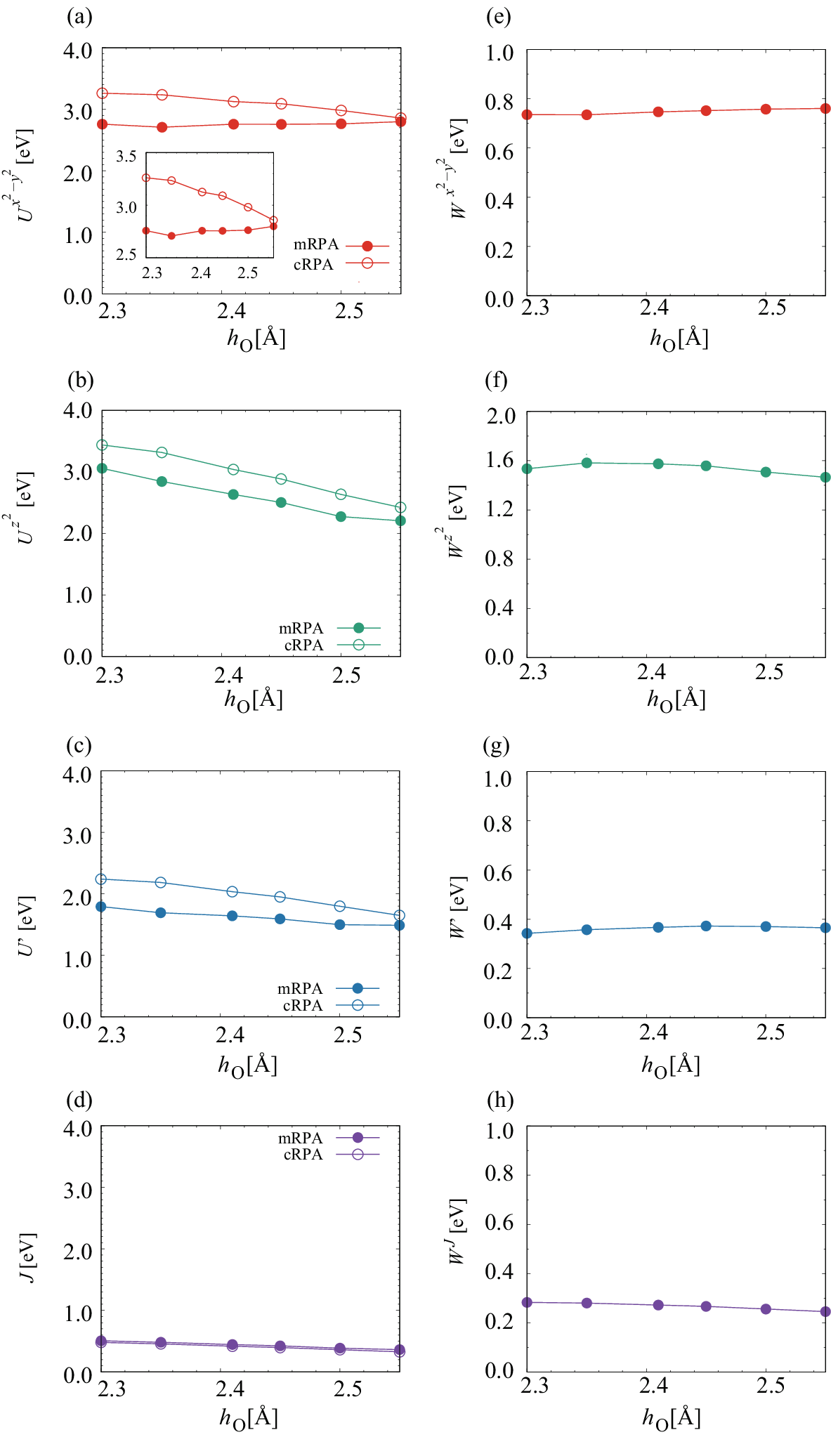
Our mRPA and cRPA results are rather different. In Ref. Jang et al. 2016, we treated a variety of layered cuprates, where we show that the effective interaction for La is larger than that for Hg as shown by $U_{\sf m}$ in Table 2, based on the cRPA calculations. In addition, we showed the effective interactions are controlled by $h_{\rm O}$ as shown in $U_{\sf m}$ in Fig. 3. Even though we do not need to modify the overall conclusion in Ref. Jang et al. 2016, we should not take such effective interactions as suitable for Hubbard models. Along the logic of mRPA, we should use $U_{\sf M}$ instead of $U_{\sf m}$.

For the model Hamiltonian $\widehat{H}_{\sf M}$ obtained from mRPA, we perform two-orbital FLEX calculations to obtain dressed Green’s functions $G_{ij}(k)$ Bickers et al. 1989; Lichtenstein and Katsnelson 1998; Yada and Kontani 2005; Mochizuki et al. 2005; Takimoto et al. 2004. Here $k=({\bm{k}},i\omega_{n})$ is a composite index made of the wave vector $\bm{k}$ and the Matsubara frequency $i\omega_{n}$. The band index $i$ takes 1 or 2. We calculate only the optimally doped case for $T_{c}$ (15% doping). We take $32\times 32\times 4$ $k$-meshes and 1024 Matsubara frequencies.

Let us remind step (3) in Fig. 1 to determine the counter one-body term $\bar{U}_{\sf M}$. Instead of LDA, let us consider QSGW case first. Theoretically, it is easier since QSGW is a method directly applicable even to a model Hamiltonian, where QSGW determines a mean-field one-body Hamiltonian for the model. We first determine $\widehat{H}^{0}_{\sf M}$ in QSGW by the first-principle QSGW calculation and the Wannier function method in the step (1) of mRPA. Then we can determine $\widehat{U}_{\sf M}$ in the step (2) of mRPA. In the step (3), we apply the QSGW method to the model Hamiltonian $\widehat{H}_{\sf M}=\widehat{H}^{0}_{\sf M}+\widehat{U}_{\sf M}-\bar{U}_{\sf M}$, where yet unknown term $\bar{U}_{\sf M}$ is included. Here $\bar{U}_{\sf M}$ is determined so that the QSGW applied to $H_{\sf M}$ do give the mean-field one-body Hamiltonian $\widehat{H}^{0}_{\sf M}$. That is, the effect of $\widehat{U}_{\sf M}$ to the one-body Hamiltonian is completely canceled by $\bar{U}_{\sf M}$.

When we start from LDA instead of QSGW, we have no unique way to determine $\bar{U}_{\sf M}$ since LDA cannot be applicable to the model Hamiltonian. Thus we need some assumption to follow the case of QSGW. Here we identify the static part of the self-energy $\Sigma(\bm{k},0)$ as $\bar{U}_{\sf M}$ (our definition of $\Sigma(\bm{k},0)$ here includes the Hartree term). In other words, if we perform a static FLEX calculation only with $\Sigma(\bm{k},0)$, we reproduce the one-body Hamiltonian of LDA. This method is equivalent to Eq. (5) in Ref. Ikeda et al. 2010. We simply assume FLEX is not for the mean-field part, but for the $\omega-$dependent self-energy part.

Here we investigate superconductivity in the two-orbital model. By substituting $G_{ij}(k)$ into the linearized Eliashberg equation,

we obtain the gap function $\Delta_{ij}(k)$ as an eigenstate and its eigenvalue $\lambda$, where $V(q)$ is the singlet pairing interaction as described in Eq. (2)-(7) of Ref. Sakakibara et al. 2012a. The largest $\lambda$ reaches unity at $T=T_{c}$. Since $\lambda$ is monotonic and increasing function of $T^{-1}$, we use $\lambda$ at $T=0.01$ eV as a qualitative measure of $T_{c}$ instead of calculating at $T_{c}$. In some FLEX calculations, $\lambda$ at fixed temperature is used to compare relative height of $T_{c}$ among similar materials Kuroki et al. 2009; Ikeda et al. 2010. We obtain $\lambda=0.50$ for La and 0.71 for Hg. This is qualitatively consistent with the experimental observation that Hg ($T_{c}=98$ K) is higher than La ($T_{c}=39$ K) Takagi et al. 1992; Yamamoto et al. 2002.

To investigate how $U_{\sf M}$ affects $\lambda$ in more detail, we perform calculations by rescaling $U_{\sf M}$ hypothetically. We plot $\lambda$ as a function of $U^{x^{2}-y^{2}}$ in Fig. 4. In the calculation, $\widehat{H}^{0}_{\sf M}$ and the ratio between all the elements of $U_{\sf M}$ are fixed. We see that $\lambda$ increases rapidly with smaller $U^{x^{2}-y^{2}}$ and plateaus with larger $U^{x^{2}-y^{2}}$ in both materials. The cases of original $U^{x^{2}-y^{2}}$ as shown in table 2 are shown by open circles. These are in the plateau region ³³ 3 The correlation between $U/t$ and $T_{c}$ is discussed with Hubbard model calculations, e.g., in Ref. Yokoyama et al. 2013.. Because of the small changes in the region, $\lambda$ of the two cuprates do not change so much even if we use $U_{\sf m}$ instead of $U_{\sf M}$, where $\lambda_{\sf cRPA}^{\sf La}=0.52$ and $\lambda_{\sf cRPA}^{\sf Hg}=0.64$. The difference between La and Hg is mainly from the hybridization of the $d_{x^{2}-y^{2}}$ orbital with the $d_{z^{2}}$ orbital. This is already examined by previous FLEX calculations with empirically determined interaction parameters Sakakibara et al. 2010. Sakakibara et al. already showed that FLEX reproduces the experimental trends of $T_{c}$ (see Fig. 1(a) of Ref. Sakakibara et al. 2014). The detailed mechanism how the hybridization affects $T_{c}$ was discussed in Sec. III D of Ref. Sakakibara et al. 2012a.

With mRPA, we obtain the two-orbital Hubbard models for La₂CuO₄ and HgBa₂CuO₄ in first-principles. The main part of mRPA is how to determine the on-site interaction parametrized by four parameters. We see that the interactions are close to those in cRPA. However, we see some differences. A difference comes from the fact that the effective size of the polarization function $P_{\sf m}$ in cRPA becomes smaller than $P_{\sf M}$ in mRPA. This is because that the probability factors $c_{i}$ in Eq. ​(8) are distributed among the oxygen bands when $d$-$p$ hybridization is strong, as in HgBa₂CuO₄.

For the models, we perform FLEX to evaluate superconductivity. The results are consistent with experiments. With the interaction obtained in mRPA, we confirm that $T_{c}$ is not so strongly dependent on the scale of interaction. Along the line of the combination of mRPA and FLEX, we will be able to predict new superconductors.

We appreciate discussions with Drs. Friedlich, Şaşıoǧlu, Imada, Arita, Hirayama, Kuroki, S. W. Jang, and M. J. Han. H.S. appreciates fruitful discussions with Drs. Misawa, Nomura, and Shinaoka. This work was supported by JSPS KAKENHI (Grant No. 16K21175, 17K05499). The computing resource is supported by Computing System for Research in Kyushu University (ITO system), the supercomputer system in RIKEN (HOKUSAI), and the supercomputer system in ISSP (sekirei).

References

- Honerkamp (2012) C. Honerkamp, Phys. Rev. B 85, 195129 (2012).
- Kinza and Honerkamp (2015) M. Kinza and C. Honerkamp, Phys. Rev. B 92, 045113 (2015).
- White (1992) S. R. White, Phys. Rev. Lett. 69, 2863 (1992).
- Gull et al. (2011) E. Gull, A. J. Millis, A. I. Lichtenstein, A. N. Rubtsov, M. Troyer, and P. Werner, Rev. Mod. Phys. 83, 349 (2011).
- Ceperley et al. (1977) D. Ceperley, G. V. Chester, and M. H. Kalos, Phys. Rev. B 16, 3081 (1977).
- Georges et al. (1996) A. Georges, G. Kotliar, W. Krauth, and M. J. Rozenberg, Rev. Mod. Phys. 68, 13 (1996).
- Y.M. Vilk and A.-M.S. Tremblay (1997) Y.M. Vilk and A.-M.S. Tremblay, J. Phys. I France 7, 1309 (1997).
- Kyung et al. (2003) B. Kyung, J.-S. Landry, and A.-M. S. Tremblay, Phys. Rev. B 68, 174502 (2003).
- Onari and Kontani (2012) S. Onari and H. Kontani, Phys. Rev. Lett. 109, 137001 (2012).
- Tsuchiizu et al. (2015) M. Tsuchiizu, Y. Yamakawa, S. Onari, Y. Ohno, and H. Kontani, Phys. Rev. B 91, 155103 (2015).
- Bickers et al. (1989) N. E. Bickers, D. J. Scalapino, and S. R. White, Phys. Rev. Lett. 62, 961 (1989).
- Sakakibara et al. (2017) H. Sakakibara, S. W. Jang, H. Kino, M. J. Han, K. Kuroki, and T. Kotani, J. Phys. Soc. Jpn. 86, 044714 (2017).
- Marzari and Vanderbilt (1997) N. Marzari and D. Vanderbilt, Phys. Rev. B 56, 12847 (1997).
- Souza et al. (2001) I. Souza, N. Marzari, and D. Vanderbilt, Phys. Rev. B 65, 035109 (2001).
- Kotani (2000) T. Kotani, J. Phys. Condens. Matter 12, 2413 (2000).
- Aryasetiawan et al. (2004) F. Aryasetiawan, M. Imada, A. Georges, G. Kotliar, S. Biermann, and A. I. Lichtenstein, Phys. Rev. B 70, 195104 (2004).
- Nakamura et al. (2008) K. Nakamura, R. Arita, and M. Imada, J. Phys. Soc. Jpn. 77, 093711 (2008).
- Nakamura et al. (2009) K. Nakamura, Y. Yoshimoto, T. Kosugi, R. Arita, and M. Imada, J. Phys. Soc. Jpn. 78, 083710 (2009).
- Miyake et al. (2009) T. Miyake, F. Aryasetiawan, and M. Imada, Phys. Rev. B 80, 155134 (2009).
- Miyake et al. (2010) T. Miyake, K. Nakamura, R. Arita, and M. Imada, J. Phys. Soc. Jpn. 79, 044705 (2010).
- Nakamura et al. (2010) K. Nakamura, Y. Yoshimoto, Y. Nohara, and M. Imada, J. Phys. Soc. Jpn. 79, 123708 (2010).
- Wehling et al. (2011) T. O. Wehling, E. Şaşıoğlu, C. Friedrich, A. I. Lichtenstein, M. I. Katsnelson, and S. Blügel, Phys. Rev. Lett. 106, 236805 (2011).
- Şaşıoǧlu et al. (2011) E. Şaşıoǧlu, C. Friedrich, and S. Blügel, Phys. Rev. B 83, 121101 (2011).
- Misawa et al. (2012) T. Misawa, K. Nakamura, and M. Imada, Phys. Rev. Lett. 108, 177007 (2012).
- Nomura et al. (2012) Y. Nomura, M. Kaltak, K. Nakamura, C. Taranto, S. Sakai, A. Toschi, R. Arita, K. Held, G. Kresse, and M. Imada, Phys. Rev. B 86, 085117 (2012).
- Nakamura et al. (2012) K. Nakamura, Y. Yoshimoto, and M. Imada, Phys. Rev. B 86, 205117 (2012).
- Shinaoka et al. (2012) H. Shinaoka, T. Misawa, K. Nakamura, and M. Imada, J. Phys. Soc. Jpn. 81, 034701 (2012).
- Werner et al. (2012) P. Werner, M. Casula, T. Miyake, F. Aryasetiawan, A. J. J. Millis, and S. Biermann, Nat. Phys. 8, 331 (2012).
- Casula et al. (2012) M. Casula, P. Werner, L. Vaugier, F. Aryasetiawan, T. Miyake, A. J. Millis, and S. Biermann, Phys. Rev. Lett. 109, 126408 (2012).
- Misawa and Imada (2014) T. Misawa and M. Imada, Nat. Commun. 5, 6738 (2014).
- Koretsune and Hotta (2014) T. Koretsune and C. Hotta, Phys. Rev. B 89, 045102 (2014).
- Şaşıoǧlu (2014) E. Şaşıoǧlu, in Lecture Notes of the 45th IFF Spring School “Computing Solids - Models, ab initio methods and supercomputing” (Forschungszentrum Jülich, 2014).
- Shinaoka et al. (2015) H. Shinaoka, M. Troyer, and P. Werner, Phys. Rev. B 91, 245156 (2015).
- Jang et al. (2016) S. W. Jang, H. Sakakibara, H. Kino, T. Kotani, K. Kuroki, and M. J. Han, Sci. Rep. 6, 33397 (2016).
- van Roekeghem et al. (2016) A. van Roekeghem, L. Vaugier, H. Jiang, and S. Biermann, Phys. Rev. B 94, 125147 (2016).
- Hirayama et al. (2018) M. Hirayama, Y. Yamaji, T. Misawa, and M. Imada, Phys. Rev. B 98, 134501 (2018).
- Takagi et al. (1992) H. Takagi, R. J. Cava, M. Marezio, B. Batlogg, J. J. Krajewski, W. F. Peck, P. Bordet, and D. E. Cox, Phys. Rev. Lett. 68, 3777 (1992).
- Yamamoto et al. (2002) A. Yamamoto, K. Minami, W.-Z. Hu, A. Miyakita, M. Izumi, and S. Tajima, Phys. Rev. B 65, 104505 (2002).
- Sakakibara et al. (2010) H. Sakakibara, H. Usui, K. Kuroki, R. Arita, and H. Aoki, Phys. Rev. Lett. 105, 057003 (2010).
- Sakakibara et al. (2012a) H. Sakakibara, H. Usui, K. Kuroki, R. Arita, and H. Aoki, Phys. Rev. B 85, 064501 (2012a).
- Sakakibara et al. (2012b) H. Sakakibara, K. Suzuki, H. Usui, K. Kuroki, R. Arita, D. J. Scalapino, and H. Aoki, Phys. Rev. B 86, 134520 (2012b).
- Sakakibara et al. (2014) H. Sakakibara, K. Suzuki, H. Usui, S. Miyao, I. Maruyama, K. Kusakabe, R. Arita, H. Aoki, and K. Kuroki, Phys. Rev. B 89, 224505 (2014).
- Kamimura and Eto (1990) H. Kamimura and M. Eto, J. Phys. Soc. Jpn. 59, 3053 (1990).
- Eto and Kamimura (1991) M. Eto and H. Kamimura, J. Phys. Soc. Jpn. 60, 2311 (1991).
- Freeman and Yu (1988) A. Freeman and J. Yu, Physica B+C 150, 50 (1988).
- Wang et al. (2011) X. Wang, H. T. Dang, and A. J. Millis, Phys. Rev. B 84, 014530 (2011).
- Hozoi et al. (2011) L. Hozoi, L. Siurakshina, P. Fulde, and J. van den Brink, Sci. Rep. 1, 65 (2011).
- Uebelacker and Honerkamp (2012) S. Uebelacker and C. Honerkamp, Phys. Rev. B 85, 155122 (2012).
- Hozoi and Laad (2007) L. Hozoi and M. S. Laad, Phys. Rev. Lett. 99, 256404 (2007).
- Matt et al. (2018) C. E. Matt, D. Sutter, A. M. Cook, Y. Sassa, M. Månsson, O. Tjernberg, L. Das, M. Horio, D. Destraz, C. G. Fatuzzo, K. Hauser, M. Shi, M. Kobayashi, V. N. Strocov, T. Schmitt, P. Dudin, M. Hoesch, S. Pyon, T. Takayama, H. Takagi, O. J. Lipscombe, S. M. Hayden, T. Kurosawa, N. Momono, M. Oda, T. Neupert, and J. Chang, Nature Communications 9, 972 (2018).
- Jorgensen et al. (1987) J. D. Jorgensen, H. B. Schüttler, D. G. Hinks, D. W. Capone II, K. Zhang, M. B. Brodsky, and D. J. Scalapino, Phys. Rev. Lett. 58, 1024 (1987).
- Wagner et al. (1993) J. Wagner, P. Radaelli, D. Hinks, J. Jorgensen, J. Mitchell, B. Dabrowski, G. Knapp, and M. Beno, Physica C: Superconductivity 210, 447 (1993).
- (53) A first-principles electronic-structure suite based on the PMT method, ecalj package, is freely available from https://github.com/tkotani/ecalj. Its one-body part is developed based on the LMTO part in the LMsuit package at http://www.lmsuite.org/.
- Kotani et al. (2007) T. Kotani, M. van Schilfgaarde, and S. V. Faleev, Phys. Rev. B 76, 165106 (2007).
- Kotani (2014) T. Kotani, J. Phys. Soc. Jpn. 83, 094711 (2014).
- Deguchi et al. (2016) D. Deguchi, K. Sato, H. Kino, and T. Kotani, Jpn. J. Appl. Phys. 55, 051201 (2016).
- (57) In our previous paper Sakakibara et al. 2017, we made a wrong statement that would become smaller if we consider off-site interactions.
- (58) We use the tetrahedron method Kotani et al. 2007; Kotani 2014 in the Brillouin zone to calculate the matrix and , where we use -points for La2CuO4(HgBa2CuO4). For a model calculation to determine , we take -point grids for discrete summation. We use dense enough 4096 Matsubara meshes at eV (virtually equal to eV.).
- Ohta et al. (1991) Y. Ohta, T. Tohyama, and S. Maekawa, Phys. Rev. B 43, 2968 (1991).
- Andersen et al. (1995) O. Andersen, A. Liechtenstein, O. Jepsen, and F. Paulsen, Journal of Physics and Chemistry of Solids 56, 1573 (1995), proceedings of the Conference on Spectroscopies in Novel Superconductors.
- Pavarini et al. (2001) E. Pavarini, I. Dasgupta, T. Saha-Dasgupta, O. Jepsen, and O. K. Andersen, Phys. Rev. Lett. 87, 047003 (2001).
- Mori et al. (2008) M. Mori, G. Khaliullin, T. Tohyama, and S. Maekawa, Phys. Rev. Lett. 101, 247003 (2008).
- Weber et al. (2010) C. Weber, K. Haule, and G. Kotliar, Phys. Rev. B 82, 125107 (2010).
- Weber et al. (2012) C. Weber, C. Yee, K. Haule, and G. Kotliar, Europhys. Lett. 100, 37001 (2012).
- Lichtenstein and Katsnelson (1998) A. I. Lichtenstein and M. I. Katsnelson, Phys. Rev. B 57, 6884 (1998).
- Yada and Kontani (2005) K. Yada and H. Kontani, J. Phys. Soc. Jpn. 74, 2161 (2005).
- Mochizuki et al. (2005) M. Mochizuki, Y. Yanase, and M. Ogata, Phys. Rev. Lett. 94, 147005 (2005).
- Takimoto et al. (2004) T. Takimoto, T. Hotta, and K. Ueda, Phys. Rev. B 69, 104504 (2004).
- Ikeda et al. (2010) H. Ikeda, R. Arita, and J. Kuneš, Phys. Rev. B 81, 054502 (2010).
- Kuroki et al. (2009) K. Kuroki, H. Usui, S. Onari, R. Arita, and H. Aoki, Phys. Rev. B 79, 224511 (2009).
- (71) The correlation between and is discussed with Hubbard model calculations, e.g., in Ref. Yokoyama et al. 2013.
- Yokoyama et al. (2013) H. Yokoyama, M. Ogata, Y. Tanaka, K. Kobayashi, and H. Tsuchiura, J. Phys. Soc. Jpn. 82, 014707 (2013).