跳到论文正文
W Papers独立论文阅读器 arXiv:1812.03475 论文正文 计算阅读时间 · 0%
引用这篇论文根据当前论文元数据生成,正式投稿前建议核对。


License: arXiv.org perpetual non-exclusive license
arXiv:1812.03475v1 [econ.EM] 09 Dec 2018

A supreme test for periodic explosive GARCH

Stefan Richter??,??abel=e1    mark]stefan.richter@iwr.uni-heidelberg.de    Weining Wang??,??abel=e2    mark]weining.wang@city.ac.uk    Wei Biao Wu??,??abel=e3    mark]wbwu@galton.uchicago.edu
Abstract

We develop a uniform test for detecting and dating explosive behavior of a strictly stationary GARCH(r,s)(r,s) (generalized autoregressive conditional heteroskedasticity) process. Namely, we test the null hypothesis of a globally stable GARCH process with constant parameters against an alternative where there is an ’abnormal’ period with changed parameter values. During this period, the change may lead to an explosive behavior of the volatility process. It is assumed that both the magnitude and the timing of the breaks are unknown. We develop a double supreme test for the existence of a break, and then provide an algorithm to identify the period of change. Our theoretical results hold under mild moment assumptions on the innovations of the GARCH process. Technically, the existing properties for the QMLE in the GARCH model need to be reinvestigated to hold uniformly over all possible periods of change. The key results involve a uniform weak Bahadur representation for the estimated parameters, which leads to weak convergence of the test statistic to the supreme of a Gaussian Process. In simulations we show that the test has good size and power for reasonably large time series lengths. We apply the test to Apple asset returns and Bitcoin returns.

keywords
GARCH , IGARCH , Change-point Analysis , Concentration Inequalities , Uniform Test

, and

??Institut für Angewandte Mathematik, Universität Heidelberg, Im Neuenheimer Feld 205, 69120 Heidelberg, Germany. ??

??Department of Economics, City, U of London, center of applied statistics, HU Berlin, Unter den Linden 6, 10099 Berlin, Germany. ??

??Department of Statistics, University of Chicago, 5734 S. University Avenue, Chicago, IL 60637, USA. ??

1 Introduction

Volatility is an important indicator for economic and financial stability. There is a growing evidence for the unstable behavior of the historical volatility of numerous micro level as well as macro level data, such as individual stocks prices, asset returns, VIX, inflation and unemployment. [2] document the unstable behavior of higher moments of many economic variables, such as R&D (research and develop) rates related to the uncertainty about future productivity. It is understood that the nature of uncertainty is the unpredictability of any model to the future path of a time series. Therefore it may be connected with a change of the parameter values in the underlying data generating process. A direct empirical fact is that one often sees a sudden explosive behavior in the second moment of the process which bounces back after a while. For example, in Figure 1 we have plotted a realization of a piece-wise explosive GARCH(1,1) process and the log returns of Bitcoin. The whole time span is set to be (July 28, 2010- May 14, 2011) with an explosive period with changing parameter values (December 30, 2010 - October 15, 2011). The two trajectories of the time series look rather similar. Such kind of data phenomena suggest that the underlying processes have time varying parameters, calling for a rigorous econometric treatment for detection of change periods and corresponding inference. We see that the piecewise explosive GARCH process in Figure 1 captures the explosive behavior of Bitcoin in the squared returns. The aim of our paper is to develop a generalised supreme test for GARCH models which is able to detect exuberance behaviour periods (periods with explosive parameter values) which are associated with the empirical phenomena of explosiveness in the second moment.

Figure 1: Plot of simulated piecewise explosive squared returns (upper panel) versus Bitcoin squared log returns (lower panel). A stable period (20100728- 20110514) versus an explosive period (20100901-20110301).

The highly celebrated autoregressive conditional heteroskedasticity (ARCH) model proposed by [6] is important for describing the pervasive phenomena of heteroskedasticity presented in many time series. One key generalization of ARCH is the GARCH model, i.e.

Xi2\displaystyle X_{i}^{2} =\displaystyle= ζi2​σi2,\displaystyle\zeta_{i}^{2}\sigma_{i}^{2},
σi2\displaystyle\sigma_{i}^{2} =\displaystyle= α0+∑j=1rαj​Xi−j2+∑k=1sβk​σi−k2,\displaystyle\alpha_{0}+\sum_{j=1}^{r}\alpha_{j}X_{i-j}^{2}+\sum_{k=1}^{s}\beta_{k}\sigma_{i-k}^{2}, (1)

where the conditional variance σi2\sigma_{i}^{2} depends on the past observations Xi−j2X_{i-j}^{2} but also on the historical conditional variance σi−k2\sigma_{i-k}^{2}. ζi\zeta_{i} are assumed to be i.i.d. innovations, see for example [16] for more details of the model.

Numerous estimation methods for the parameters of GARCH models have been proposed, and the consistency and asymptotic normality has been carefully studied in the literature. A conventional estimation approach is the quasi maximum likelihood estimation (QMLE), e.g. [3]. Also [7] study quasi-maximum likelihood estimation of GARCH models with heavy-tailed likelihoods. [17] propose a least absolute deviation estimator. [12] establish consistency and asymptotic normality of the quasi-maximum likelihood estimator in the linear ARCH model. It is well known that under the assumption of strict stationarity of a GARCH model, there is still a region of parameter values allowing for realizations with unstable volatility behavior. The leading case is the “IGARCH" process. [15] looks at the behavior of an “IGARCH" process, and it is known that the unconditional mean of the IGARCH’s conditional variance is not finite, which implies infinite second or higher moments (i.e. eruptive behavior). [14] provide an asymptotic theory for a strictly stationary GARCH(1,1) quasi-maximum likelihood estimator allowing for the case of IGARCH and explosive conditional variance and even nonstationarity. [12] consider asymptotic inference for nonstationary GARCH model.

Despite the rich empirical literature which suggests the existence of an unstable moment period of a GARCH process, there is only sparse literature on determining and testing the period of explosiveness. [9] provide a test for testing strict stationarity of a GARCH(1,1) process. Their results however do not lead to a handy tool for checking for the existence of an explosive period and determining its range. There is also a large and important literature on testing for explosiveness and dating the period of instability in the price or dividend processes of a financial asset using a supreme unit root test for bubbles. See for example [18] for a left-tailed augmented Dickey-Fuller test (ADF) for the explosive behavior in the 1990s Nasdaq. [10] considers such kind of bubble tests for crypto-currencies. [11] investigate a bubble test with a smooth time varying volatility function. The underlying models focus usually on unit root or explosive auto-regressive (AR) processes to test the change of the AR(1) coefficient. Often the variance of the errors stays the same or vary smoothly after the explosion which means that the volatility increase is mostly driven by the increase of the AR parameter. In our model we choose a different approach to model an explosion of volatility: we describe the evolution of the data-generating process by a GARCH process and therefore link the source of a change in the volatility to a change of the parameters in the volatility recursion.

It is worth noting that unlike a bubble test for an AR process, it is quite debatable to link a direct cause of the bursting behavior to the volatility process, see [13]. In contrary, volatility bursting can also be related to time varying risk aversion, sentiment, bubble or uncertainty. Nevertheless, we are trying to establish a theoretical rigorous framework of testing for the explosive interval using a GARCH model for the volatility process. It should be stressed that we focus on one aspect of the parameter and model uncertainty, namely changes in the parameters driving the volatility over time. We do not claim that our method can directly identify the cause of this behavior. In sum, we develop a change-point test for detecting possible unstable behavior of a strictly stationary GARCH(r,s)(r,s) process. The null hypothesis is a GARCH process with globally constant parameters while the alternative is the existence of a period where the parameter values change to another (higher) value. This increase potentially leads to a period of explosive volatility.

Assuming that no information on the period and the change itself is available, we develop a test statistic based on supremes which searches over all possible sub-windows of the data. We prove asymptotic consistency and provide a limit distribution of our test statistic. It is important that the test is not of unit-root-type since hypothesis and alternative are still in the regime where the GARCH process is strictly stationary. The theoretical contributions are uniform consistency statements of the QML estimators over an arbitrary observation period, a uniform weak Bahadur representation and corresponding uniform distributional limit results. For the proofs we carve out the essential analytical properties of the likelihood functions and use new concentration inequalities from [23] leading to mild moment assumptions.

We introduce some notations we use throughout the paper. For q>0q>0 and vector v=(v1,…,vd)⊤∈ℝd,v=(v_{1},\ldots,v_{d})^{\top}\in\mathbb{R}^{d}, let |v|1:=∑i=1d|vi||v|_{1}:=\sum_{i=1}^{d}|v_{i}|. For matrices A∈ℝd×dA\in\mathbb{R}^{d\times d}, we similarly use |A|1:=s​u​mi,j=1d​|Ai,j||A|_{1}:=sum_{i,j=1}^{d}|A_{i,j}|. We denote by |A|2=max|v|=1⁡|A​v|2|A|_{2}=\max_{|v|=1}|Av|_{2} the spectral norm of AA. We use Zn​→𝑑​ZZ_{n}\overset{d}{\to}Z and Zn​→𝑝​ZZ_{n}\overset{p}{\to}Z to denote convergence in distribution and convergence in probability for random variables Zn,ZZ_{n},Z. For some sequence (yj)j∈ℕ(y_{j})_{j\in\mathbb{N}} of real numbers and some sequence (χj)j∈ℕ(\chi_{j})_{j\in\mathbb{N}} of nonnegative real numbers, define the weighted seminorm

|y|χ,q:=(∑j=1∞χj​|yj|q)1/q.|y|_{\chi,q}:=\Big(\sum_{j=1}^{\infty}\chi_{j}|y_{j}|^{q}\Big)^{1/q}.

For some sequences (an)(a_{n}) and (bn)(b_{n}) of positive numbers, write an=O⁡(bn)a_{n}=O(b_{n}) or an=o⁡(bn)a_{n}=o(b_{n}) if there exists a positive constant CC such that an/bn≤Ca_{n}/b_{n}\leq C or an/bn→0a_{n}/b_{n}\rightarrow 0 respectively. For two sequences of random variables (Xn)(X_{n}) and (Yn),(Y_{n}), write Xn=op​(Yn)X_{n}=o_{p}(Y_{n}) (resp. Xn=Op​(Yn)X_{n}=O_{p}(Y_{n})) if Xn/Yn→0X_{n}/Y_{n}\rightarrow 0 in probability (Xn/YnX_{n}/Y_{n} is bounded in probability). For some random variable ZZ, define ‖Z‖q:=(𝔼​|Z|q)1/q\|Z\|_{q}:=(\mathbb{E}|Z|^{q})^{1/q}. If ∥⋅∥q\|\cdot\|_{q} is applied to a matrix, this is meant by a component-wise operation. For the i.i.d. random variables ζi\zeta_{i}, i∈ℤi\in\mathbb{Z} used in the model definition (5), let ℱi:=(ζi,ζi−1,…)\mathcal{F}_{i}:=(\zeta_{i},\zeta_{i-1},...). With some abuse of notation, we refer to ℱi\mathcal{F}_{i} also as the σ\sigma algebra generated by the entries of ℱi\mathcal{F}_{i}. For Xi=h⁡(ℱi)X_{i}=h(\mathcal{F}_{i}), i∈ℤi\in\mathbb{Z} with some measurable function hh, we define the functional dependence measure (cf. [21]),

δq​(k):=‖Xi−Xi∗‖q,\delta_{q}(k):=\|X_{i}-X_{i}^{*}\|_{q},

where Xi∗=h⁡(ℱi∗)X_{i}^{*}=h(\mathcal{F}_{i}^{*}) and ℱi∗:=(ζi,…,ζ1,ζ0∗,ζ−1,ζ−2,…)\mathcal{F}_{i}^{*}:=(\zeta_{i},...,\zeta_{1},\zeta_{0}^{*},\zeta_{-1},\zeta_{-2},...) with ζ0∗\zeta_{0}^{*} being an independent copy of ζ0\zeta_{0}.

Our text is organized as follows. Section 2 provides the results for the important GARCH(1,1) model and the corresponding test procedure. Section 3 is concerning the estimation and theoretical results in a general GARCH(r,sr,s) model. In particular, Section 3.1 introduces the framework of the QMLE and the consistency of the QMLE, and Section 3.2 presents the theoretical foundations of our uniform test and discusses the estimation of the covariance matrix of the QMLE appearing in the test statistic. In Section 4 we analyze the size and the power of our test in simulations, while Section 5 discusses the behavior of the test in examples from practice. The technical proofs are delegated to the Appendix.

2 A supreme explosiveness test for GARCH(1,1)

In this section, we introduce our model by starting with a simple testing framework for the GARCH(1,1) model. Then we will provide a rigorous theoretical treatment by starting with a more general GARCH(r,sr,s) model in the following section. We consider first of all the baseline GARCH(1,1) model over the whole sample period with possibly time-varying parameters,

Xi\displaystyle X_{i} =\displaystyle= ζi​σi,\displaystyle\zeta_{i}\sigma_{i},
σi2\displaystyle\sigma_{i}^{2} =\displaystyle= α0​(i)+α1​(i)​Xi−12+β1​(i)​σi−12,i∈ℤ,\displaystyle\alpha_{0}(i)+\alpha_{1}(i)X_{i-1}^{2}+\beta_{1}(i)\sigma_{i-1}^{2},\quad i\in\mathbb{Z}, (2)

where ζi\zeta_{i} is an i.i.d. sequence of random variables with 𝔼​ζ1=0\mathbb{E}\zeta_{1}=0, 𝔼​ζ12=1\mathbb{E}\zeta_{1}^{2}=1, and α0​(i),α1​(i),β1​(i)>0\alpha_{0}(i),\alpha_{1}(i),\beta_{1}(i)>0 are the underlying parameters at each time point. We collect data of this model at time points 1,…,n1,\dots,n.

We summarize the parameters into θ⁡(i)=(α0​(i),α1​(i),β1​(i))′\theta(i)=(\alpha_{0}(i),\alpha_{1}(i),\beta_{1}(i))^{\prime}. In the case that the parameters are constant, i.e. θ⁡(i)≡θ=(α0′,α1′,β1′)′\theta(i)\equiv\theta=(\alpha_{0}^{\prime},\alpha_{1}^{\prime},\beta_{1}^{\prime})^{\prime}, the top Lyapunov exponent associated with this model according to [5] is

γ⁡(θ)=𝔼​log⁡(α1​ζ12+β1).\gamma(\theta)=\mathbb{E}\log(\alpha_{1}\zeta_{1}^{2}+\beta_{1}).

It is worth noting that γ⁡(θ)<0\gamma(\theta)<0 allows (for instance) the IGARCH case, i.e. α1+β1=1\alpha_{1}+\beta_{1}=1. The aim of this paper is to construct tests for a period of changed parameters in the GARCH model, which allows for the explosiveness of the variances of the process. Namely, we would like to test whether there exists a period {n1,…,n2}\{n_{1},...,n_{2}\} (with 1<n1<n2<n1<n_{1}<n_{2}<n), where the parameter values in (2) change there values compared with {1,…,n}\{1,...,n\}. The task breaks into two parts: First, checking for the existence of a change, for which a uniform test is needed. Second, one has to identify the period of the change and to estimate the corresponding parameters.

For our studies, let

Θ={θ=(α0,α1,β1)∈ℝ3:γ⁡(θ)​<0,α0,α1,β1>​0}\Theta=\{\theta=(\alpha_{0},\alpha_{1},\beta_{1})\in\mathbb{R}^{3}:\gamma(\theta)<0,\alpha_{0},\alpha_{1},\beta_{1}>0\}

be the parameter space which contains all possible configurations of θ=(α0,α1,β1)\theta=(\alpha_{0},\alpha_{1},\beta_{1}).

Let θ∗​(i)=(α0∗​(i),α1∗​(i),β1∗​(i))′\theta^{*}(i)=(\alpha_{0}^{*}(i),\alpha_{1}^{*}(i),\beta_{1}^{*}(i))^{\prime} denote the true parameter in the baseline model, which possibly has a period of change in {⌊n​τ1∗⌋+1,…,⌊n​τ2∗⌋}\{\lfloor n\tau_{1}^{*}\rfloor+1,...,\lfloor n\tau_{2}^{*}\rfloor\} (where τ1∗,τ2∗∈[0,1]\tau_{1}^{*},\tau_{2}^{*}\in[0,1], τ1∗<τ2∗\tau_{1}^{*}<\tau_{2}^{*}) with a magnitude Δ∗=[δ1∗,δ2∗,δ3∗]′\Delta^{*}=[\delta_{1}^{*},\delta_{2}^{*},\delta_{3}^{*}]^{\prime}. Namely,

θ∗​(i)={θ∗,i≤⌊n​τ1∗⌋,θ∗+Δ∗,⌊n​τ1∗⌋+1≤i≤⌊n​τ2∗⌋,θ∗,i>⌊n​τ2∗⌋.\theta^{*}(i)=\begin{cases}\theta^{*},&i\leq\lfloor n\tau_{1}^{*}\rfloor,\\ \theta^{*}+\Delta^{*},&\lfloor n\tau_{1}^{*}\rfloor+1\leq i\leq\lfloor n\tau_{2}^{*}\rfloor,\\ \theta^{*},&i>\lfloor n\tau_{2}^{*}\rfloor.\end{cases}

Here ⌊x⌋\lfloor x\rfloor denotes the flooring operator, i.e. the largest integer smaller or equal to xx. An interesting question is to test whether the process is stable, i.e. α1∗​(i)+β1∗​(i)<1\alpha_{1}^{*}(i)+\beta_{1}^{*}(i)<1 for all time points i=1,…,ni=1,...,n versus the hypothesis that there exists a period explosiveness in which α1∗​(i)+β1∗​(i)>1\alpha^{*}_{1}(i)+\beta^{*}_{1}(i)>1 for some ii. α1∗​(i)+β1∗​(i)\alpha_{1}^{*}(i)+\beta_{1}^{*}(i) is referred to as the persistency parameter in our setting. Graphically, this corresponds to the question if there exists regions where the process leaves the variance-stationary regime (i.e. the variance explodes).

We formulate our hypothesis therefore in the following way, with α1∗+β1∗=c\alpha_{1}^{*}+\beta_{1}^{*}=c (c≤1c\leq 1),

H0:δ2∗+δ3∗=0v.s.H1:δ2∗+δ3∗>0.H_{0}:\delta^{*}_{2}+\delta_{3}^{*}=0\quad\text{v.s.}\quad H_{1}:\delta_{2}^{*}+\delta^{*}_{3}>0.

To construct a test, we first derive estimators for the parameters. If the period described by τ1∗,τ2∗\tau_{1}^{*},\tau_{2}^{*} is known, we can use a standard quasi maximum likelihood estimation approach. It is not hard to see from (2), that in the case of constant parameters θ⁡(i)≡θ\theta(i)\equiv\theta,

σi2=α0/(1−β1)+α1​∑k=1∞β1k​Xi−1−k2a.s.\sigma_{i}^{2}=\alpha_{0}/(1-\beta_{1})+\alpha_{1}\sum^{\infty}_{k=1}\beta_{1}^{k}X^{2}_{i-1-k}\quad\text{a.s.}

The truncated version which can be calculated from a sample is

σi2​c=α0/(1−β1)+α1​∑k=1i−2β1k​Xi−1−k2.\sigma_{i}^{2c}=\alpha_{0}/(1-\beta_{1})+\alpha_{1}\sum^{i-2}_{k=1}\beta_{1}^{k}X^{2}_{i-1-k}.

The quasi likelihood approach is to use the negative log likelihood function

Ln,τ1,τ2c​(θ):=1n​∑i=⌊n​τ1⌋+1⌊n​τ2⌋ℓ⁡(Xi2,Yic,θ),L_{n,\tau_{1},\tau_{2}}^{c}(\theta):=\frac{1}{n}\sum_{i=\lfloor n\tau_{1}\rfloor+1}^{\lfloor n\tau_{2}\rfloor}\ell(X_{i}^{2},Y_{i}^{c},\theta),

where Yic:=(Xi−12,…,X12,0,0,…)Y_{i}^{c}:=(X_{i-1}^{2},...,X_{1}^{2},0,0,...) and

ℓ⁡(Xi2,Yic,θ):=12​(Xi2σi2​c+log⁡σi2​c).\ell(X_{i}^{2},Y_{i}^{c},\theta):=\frac{1}{2}\Big(\frac{X_{i}^{2}}{\sigma_{i}^{2c}}+\log\sigma_{i}^{2c}\Big).

The estimated parameter with observations during any given period {⌊n​τ1⌋+1,…,⌊n​τ2⌋}\{\lfloor n\tau_{1}\rfloor+1,...,\lfloor n\tau_{2}\rfloor\} is defined to be θ^n,τ1,τ2=argminθ∈Θ⁡Ln,τ1,τ2c​(θ).\hat{\theta}_{n,\tau_{1},\tau_{2}}=\argmin_{\theta\in\Theta}L_{n,\tau_{1},\tau_{2}}^{c}(\theta). It can be shown that under regularity conditions, θ^n,τ1,τ2\hat{\theta}_{n,\tau_{1},\tau_{2}} is asymptotically normal with covariance matrix

Σ=V​(θ∗)−1​I​(θ∗)​V​(θ∗)−1,\Sigma=V(\theta^{*})^{-1}I(\theta^{*})V(\theta^{*})^{-1}, (3)

where

V⁡(θ):=𝔼⁡[∇θ2​ℓ​(Xi2,Yi,θ)],V(\theta):=\mathbb{E}[\nabla_{\theta}^{2}\ell(X_{i}^{2},Y_{i},\theta)],

and

I⁡(θ):=𝔼⁡[∇θℓ​(Xi2,Yi,θ)⋅∇θℓ​(Xi2,Yi,θ)′].I(\theta):=\mathbb{E}[\nabla_{\theta}\ell(X_{i}^{2},Y_{i},\theta)\cdot\nabla_{\theta}\ell(X_{i}^{2},Y_{i},\theta)^{\prime}].

Now we turn to our first step, i.e. a uniform test of the existence of the period of change. For given τ1,τ2\tau_{1},\tau_{2}, the test statistic associated with our hypothesis H0H_{0} of interest is

Tτ1,τ2=(τ2−τ1)χ(H′Σ¯n,τ1,τ2H)−1/2{α^1,n,τ1,τ2+β^1,n,τ1,τ2−c},T_{\tau_{1},\tau_{2}}=(\tau_{2}-\tau_{1})^{\chi}(H^{\prime}\bar{\Sigma}_{n,\tau_{1},\tau_{2}}H)^{-1/2}\{\hat{\alpha}_{1,n,\tau_{1},\tau_{2}}+\hat{\beta}_{1,n,\tau_{1},\tau_{2}}-c\},

where χ\chi is a scaling factor chosen for numerical stability, α^1,n,τ1,τ2\hat{\alpha}_{1,n,\tau_{1},\tau_{2}}, β^1,n,τ1,τ2\hat{\beta}_{1,n,\tau_{1},\tau_{2}} are the second and third component of θ^n,τ1,τ2\hat{\theta}_{n,\tau_{1},\tau_{2}}, and Σ¯n,τ1,τ2\bar{\Sigma}_{n,\tau_{1},\tau_{2}} is an estimator of Σ\Sigma using observations outside {⌊n​τ1⌋,…,⌊n​τ2⌋}\{\lfloor n\tau_{1}\rfloor,...,\lfloor n\tau_{2}\rfloor\}.

For instance, we can set χ=0.5\chi=0.5, Σ¯n,τ1,τ2\bar{\Sigma}_{n,\tau_{1},\tau_{2}} to be the standard covariance matrix estimator obtained by replacing V,IV,I with their empirical counterparts (see (10) below) with observations outside {⌊n​τ1⌋,…,⌊n​τ2⌋}\{\lfloor n\tau_{1}\rfloor,...,\lfloor n\tau_{2}\rfloor\} and H=(0,1,1)⊤H=(0,1,1)^{\top}.

The feasible search set is defined to be Rκ,κ′:={(τ1,τ2)∈[0,1]2:τ1<τ2,1−κ′≥τ2−τ1≥κ}R_{\kappa,\kappa^{\prime}}:=\{(\tau_{1},\tau_{2})\in[0,1]^{2}:\tau_{1}<\tau_{2},1-\kappa^{\prime}\geq\tau_{2}-\tau_{1}\geq\kappa\} (with some κ,κ′>0\kappa,\kappa^{\prime}>0, for instance κ=κ′=0.1\kappa=\kappa^{\prime}=0.1), ensuring proper estimation of Σ\Sigma due to 1−κ′≥τ2−τ11-\kappa^{\prime}\geq\tau_{2}-\tau_{1} and a change detection based on enough samples due to τ2−τ1≥κ.\tau_{2}-\tau_{1}\geq\kappa. The supreme of n​Tτ1,τ2\sqrt{n}T_{\tau_{1},\tau_{2}} converges asymptotically to the supreme of a Gaussian process, namely {B⁡(τ2)−B⁡(τ1)(τ2−τ1)1−χ}\{\frac{B(\tau_{2})-B(\tau_{1})}{(\tau_{2}-\tau_{1})^{1-\chi}}\}, where B(.)B(.) is a 1−1-dimensional Brownian motion. We show this formally in Theorem 3.9 in Section 3.2.

Empirically, we cannot exhaust all the values (τ1,τ2)∈Rκ,κ′(\tau_{1},\tau_{2})\in R_{\kappa,\kappa^{\prime}}. We therefore need to restrict the calculation of the supreme to a set of grid points as an approximation to our supreme test statistics.

We summarize our uniform test as follows.

  1. Step 0

    Choose some L>0L>0 (number of grids associated with detection accuracy). The corresponding grid points are 𝒢={jL:j=0,…,L}\mathcal{G}=\{\frac{j}{L}:j=0,...,L\} on the time line.

  2. Step 1

    Let H=(0,1,1)′H=(0,1,1)^{\prime}.

  3. Step 2

    Choose values for κ,κ′∈(0,1)\kappa,\kappa^{\prime}\in(0,1), and χ∈(0,1)\chi\in(0,1).

  4. Step 3

    For each given interval (τ1,τ2)∈Rκ,κ′∩𝒢2(\tau_{1},\tau_{2})\in R_{\kappa,\kappa^{\prime}}\cap\mathcal{G}^{2}, determine the associated QLME θ^n,τ1,τ2\hat{\theta}_{n,\tau_{1},\tau_{2}} defined in (8) and calculate Σ¯n,τ1,τ2\bar{\Sigma}_{n,\tau_{1},\tau_{2}} as in (10). Then we can calculate the test statistics as

    B^n(τ1,τ2):=n(τ2−τ1)χ{H′Σ¯n,τ1,τ2H}−1/2{H′θ^n,τ1,τ2−H′θ∗}.\hat{B}_{n}(\tau_{1},\tau_{2}):=\sqrt{n}(\tau_{2}-\tau_{1})^{\chi}\{H^{\prime}\bar{\Sigma}_{n,\tau_{1},\tau_{2}}H\}^{-1/2}\big\{H^{\prime}\hat{\theta}_{n,\tau_{1},\tau_{2}}-H^{\prime}\theta^{*}\big\}.

    (cf. (11)).

  5. Step 4

    For the critical value of this test, we can approximate the quantile of the test statistics via simulation under the null hypothesis H0H_{0}: For large NN (e.g. N=10000N=10000), generate i.i.d. εi,k∼N⁡(0,1)\varepsilon_{i,k}\sim N(0,1), i=1,…,ni=1,...,n and calculate

    μ^n,k:=sup(τ1,τ2)∈Rκ,κ′∩𝒢21n​∑i=⌊n​τ1⌋+1⌊n​τ2⌋εi,k(τ2−τ1)1−χ.\hat{\mu}_{n,k}:=\sup_{(\tau_{1},\tau_{2})\in R_{\kappa,\kappa^{\prime}}\cap\mathcal{G}^{2}}\frac{1}{\sqrt{n}}\frac{\sum_{i=\lfloor n\tau_{1}\rfloor+1}^{\lfloor n\tau_{2}\rfloor}\varepsilon_{i,k}}{(\tau_{2}-\tau_{1})^{1-\chi}}.

    We define q^W,δ:=μ^n,[⌊N⋅δ⌋]\hat{q}_{W,\delta}:=\hat{\mu}_{n,[\lfloor N\cdot\delta\rfloor]}, where μ^n,[1],…,μ^n,[N]\hat{\mu}_{n,[1]},...,\hat{\mu}_{n,[N]} are the order statistics of μ^n,1,…,μ^n,N\hat{\mu}_{n,1},...,\hat{\mu}_{n,N}. Figure 2 shows how one calculates the supreme test statistics over different windows associated with the grid points.

  6. Step 5

    We can now make a test decision based on critical values from the previous steps. If

    sup(τ1,τ2)∈Rκ,κ′∩𝒢2B^n​(τ1,τ2)>q^W,δ,\sup_{(\tau_{1},\tau_{2})\in R_{\kappa,\kappa^{\prime}}\cap\mathcal{G}^{2}}\hat{B}_{n}(\tau_{1},\tau_{2})>\hat{q}_{W,\delta}, (4)

    there is a significant shock in the parameter values. In this case, one can estimate the true shock period as [τ1∗,τ2∗][\tau_{1}^{*},\tau_{2}^{*}]

    (τ^1,n,τ^2,n)∈argmax(τ1,τ2)∈Rκ,κ′(τ2−τ1)χΣ¯n,τ1,τ2,H−1/2{H′θ^n,τ1,τ2−H′θ∗}.(\hat{\tau}_{1,n},\hat{\tau}_{2,n})\in\argmax_{(\tau_{1},\tau_{2})\in R_{\kappa,\kappa^{\prime}}}(\tau_{2}-\tau_{1})^{\chi}\bar{\Sigma}_{n,\tau_{1},\tau_{2},H}^{-1/2}\big\{H^{\prime}\hat{\theta}_{n,\tau_{1},\tau_{2}}-H^{\prime}\theta^{*}\big\}.

    If instead (4) does not hold, we conclude that there is no evidence for a period of parameter change.

  7. Step 6

    In case of the significance of our uniform test in Step 5, we re-estimate the parameter θn,τ^1,τ^2\theta_{n,\hat{\tau}_{1},\hat{\tau}_{2}}, and produce the confidence interval based on Theorem 3.9.
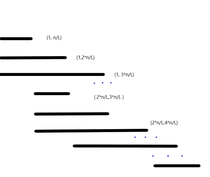
Figure 2: Plot of the windows where the supreme is calculated.
Refer to caption

We name our test as a GSRWW test (stands for GARCH supreme and the author abbreviations). The GSRWW test’s limit distribution is supτ1,τ2∈Rκ,κ′​{B⁡(τ2)−B⁡(τ1)(τ2−τ1)1−χ}\mbox{sup}_{\tau_{1},\tau_{2}\in R_{\kappa,\kappa^{\prime}}}\{\frac{B(\tau_{2})-B(\tau_{1})}{(\tau_{2}-\tau_{1})^{1-\chi}}\} (with B(.)B(.) a standard Brownian motion).

3 A supreme test for G​A​R​C​H​(r,s)GARCH(r,s)

In this section, we formulate the test and provide necessary theoretical results in a general GARCH(r,sr,s) model. For r,s∈ℕr,s\in\mathbb{N}, θ⁡(i)=(α0​(i),α1​(i),…,αr​(i),β1​(i),…,βs​(i))′\theta(i)=(\alpha_{0}(i),\alpha_{1}(i),...,\alpha_{r}(i),\beta_{1}(i),...,\beta_{s}(i))^{\prime}, we consider the GARCH(r,sr,s) model

Xi2\displaystyle X_{i}^{2} =\displaystyle= ζi2​σi2,\displaystyle\zeta_{i}^{2}\sigma_{i}^{2},
σi2\displaystyle\sigma_{i}^{2} =\displaystyle= α0​(i)+∑j=1rαj​(i)​Xi−j2+∑k=1sβk​(i)​σi−k2.\displaystyle\alpha_{0}(i)+\sum_{j=1}^{r}\alpha_{j}(i)X_{i-j}^{2}+\sum_{k=1}^{s}\beta_{k}(i)\sigma_{i-k}^{2}. (5)

Here, ζi\zeta_{i} are i.i.d. innovations with 𝔼​ζ1=0\mathbb{E}\zeta_{1}=0 and 𝔼​ζ12=1\mathbb{E}\zeta_{1}^{2}=1. We first analyze the model in the case that the parameters are constant, i.e. θ⁡(i)≡θ=(α0,α1,…,αr,β1,…,βs)′\theta(i)\equiv\theta=(\alpha_{0},\alpha_{1},...,\alpha_{r},\beta_{1},...,\beta_{s})^{\prime}. We first present our set of assumptions ensuring the existence of a unique stationary solution to our model in (5) . Define f⁡(θ)=(α1,…,αr,β1,…,βs)′f(\theta)=(\alpha_{1},\ldots,\alpha_{r},\beta_{1},\ldots,\beta_{s})^{\prime} and let ej=(0,…,0,1,0,…,0)′∈ℝr+se_{j}=(0,\ldots,0,1,0,\ldots,0)^{\prime}\in\mathbb{R}^{r+s} be the unit column vector with jjth element being 1, 1≤j≤r+s1\leq j\leq r+s. Define the (r+s)×(r+s)(r+s)\times(r+s)-matrix

Ai​(θ)=(f⁡(θ)​ζi2,e1,…,er−1,f⁡(θ),er+1,…,er+s−1)′.A_{i}(\theta)=(f(\theta)\zeta_{i}^{2},e_{1},\ldots,e_{r-1},f(\theta),e_{r+1},\ldots,e_{r+s-1})^{\prime}.

Recall that |A|2|A|_{2} is the spectral norm of a quadratic matrix AA. Define the top Lyapunov exponent of Ai​(θ)A_{i}(\theta),

γ⁡(θ):=limi→∞1i​log⁡|Ai​(θ)​Ai−1​(θ)​…​A1​(θ)|2.\gamma(\theta):=\lim_{i\to\infty}\frac{1}{i}\log|A_{i}(\theta)A_{i-1}(\theta)\dots A_{1}(\theta)|_{2}.

which exists if 𝔼​|ζ02|a<∞\mathbb{E}|\zeta_{0}^{2}|^{a}<\infty for some a>0a>0 (cf. [8]).

Assumption 3.1.

Suppose that

  1. (A1)

    ζ02\zeta_{0}^{2} has a non-degenerate distribution with 𝔼​ζ02=1\mathbb{E}\zeta_{0}^{2}=1.

  2. (A2)

    Let αm​i​n>0\alpha_{min}>0, and

    Θ~={θ∈ℝ≥0r+s+1:α0≥αm​i​n,γ(θ)<0 a.s.,∑j=1sβj<1}.\tilde{\Theta}=\{\theta\in\mathbb{R}_{\geq 0}^{r+s+1}:\alpha_{0}\geq\alpha_{min},\gamma(\theta)<0\text{ a.s.},\sum_{j=1}^{s}\beta_{j}<1\}. (6)

    Let Θ⊂Θ~\Theta\subset\tilde{\Theta} be compact. Assume that θ∗∈i​n​t​(Θ)\theta^{*}\in int(\Theta).

  3. (A3)

    Let 𝒜θ​(z):=∑i=1rαi​zi\mathcal{A}_{\theta}(z):=\sum_{i=1}^{r}\alpha_{i}z^{i}, ℬθ​(z):=1−∑j=1sβj​zj\mathcal{B}_{\theta}(z):=1-\sum_{j=1}^{s}\beta_{j}z^{j}. If s>0s>0, 𝒜θ∗​(z)\mathcal{A}_{\theta^{*}}(z) and ℬθ∗​(z)\mathcal{B}_{\theta^{*}}(z) have no common root, 𝒜θ∗​(1)≠0\mathcal{A}_{\theta^{*}}(1)\not=0 and αr∗+βs∗≠0\alpha^{*}_{r}+\beta^{*}_{s}\not=0.

Condition (A2) γ⁡(θ)<0\gamma(\theta)<0 ganrantees the strict stationarity of the GARCH process. Note that this includes parameter values corresponding to IGARCH or explosive GARCH ∑iαi+∑jβj≥1\sum_{i}\alpha_{i}+\sum_{j}\beta_{j}\geq 1.

Most of the following proposition is in the spirit of the introductory comments in [8]. However, to obtain appropriate statements for the functional dependence measure, we have to modify some arguments in the proof.

Proposition 3.2 (Existence of the GARCH model).

Let Assumption 3.1 hold. Then:

  1. (i)

    (5) has a unique stationary solution Xi2=H⁡(ℱi)X_{i}^{2}=H(\mathcal{F}_{i}), i∈ℤi\in\mathbb{Z}.

  2. (ii)

    There exists q>0q>0 with ‖X02‖q≤D\|X_{0}^{2}\|_{q}\leq D and δqX2​(k)=O⁡(ck)\delta_{q}^{X^{2}}(k)=O(c^{k}) for some 0<c<10<c<1.

  3. (iii)

    λm​a​x​(B⁡(θ))<1\lambda_{max}(B(\theta))<1, where

    B⁡(θ)=(β1β2……βs10……0010…0⋱⋱⋱0…010).B(\theta)=\begin{pmatrix}\beta_{1}&\beta_{2}&\dots&\dots&\beta_{s}\\ 1&0&\dots&\dots&0\\ 0&1&0&\dots&0\\ \vdots&\ddots&\ddots&\ddots&\vdots\\ 0&\dots&0&1&0\end{pmatrix}.

3.1 QMLE in G​A​R​C​H​(r,s)GARCH(r,s) and its consistency

In this subsection, we describe the QMLE and provide a theorem on its uniform consistency. For estimation of the parameters θ∈Θ\theta\in\Theta, we consider the following QML approach. We denote by Yic:=(Xi−12,Xi−22,…,X12,0,0,…)Y_{i}^{c}:=(X_{i-1}^{2},X_{i-2}^{2},...,X_{1}^{2},0,0,...) the observed data until time i−1i-1. For 0≤τ1<τ2≤10\leq\tau_{1}<\tau_{2}\leq 1,

Ln,τ1,τ2c​(θ):=1n​∑i=⌊n​τ1⌋+1⌊n​τ2⌋ℓ⁡(Xi2,Yic,θ),L_{n,\tau_{1},\tau_{2}}^{c}(\theta):=\frac{1}{n}\sum_{i=\lfloor n\tau_{1}\rfloor+1}^{\lfloor n\tau_{2}\rfloor}\ell(X_{i}^{2},Y_{i}^{c},\theta),

where

ℓ⁡(x,y,θ):=12​(xσ​(y,θ)2+log⁡σ​(y,θ)2)\ell(x,y,\theta):=\frac{1}{2}\Big(\frac{x}{\sigma(y,\theta)^{2}}+\log\sigma(y,\theta)^{2}\Big)

and σ​(y,θ)2\sigma(y,\theta)^{2} follows the recursion

σ​(y,θ)2=α0+∑j=1rαj​yj+∑k=1sβk​σ​((yk+1,yk+2,…),θ)2.\sigma(y,\theta)^{2}=\alpha_{0}+\sum_{j=1}^{r}\alpha_{j}y_{j}+\sum_{k=1}^{s}\beta_{k}\sigma((y_{k+1},y_{k+2},...),\theta)^{2}. (7)

The analytic definition of the recursion of σ​(y,θ)2\sigma(y,\theta)^{2} is formulated in a forward way (using y1,y2,…y_{1},y_{2},... instead of y−1y_{-1},y−2y_{-2},…) because we plug in y=Yicy=Y_{i}^{c} which is formulated in a backward way, leading to the usual quasi-likelihood approach for GARCH models. Note that σ⁡(Yic,θ)\sigma(Y_{i}^{c},\theta) in (7) terminates after a finite number of steps due to zeros in YicY_{i}^{c}. Morevoer, instead of using the truncated version Yic=(Xi−12,Xi−22,…,X12,0,…,0)Y_{i}^{c}=(X_{i-1}^{2},X_{i-2}^{2},...,X_{1}^{2},0,...,0) which corresponds to assuming that all initial values X02=X−12=…=0X_{0}^{2}=X_{-1}^{2}=...=0, one can also use different initial values like X02=X−12=…=α0X_{0}^{2}=X_{-1}^{2}=...=\alpha_{0} or X02=X−12=…=X12X_{0}^{2}=X_{-1}^{2}=...=X_{1}^{2} as investigated in [8]. For a discussion of different initial values, consider [4] (in the case of strict stationarity).

With the defined likelihood function, for 0≤τ1<τ2≤10\leq\tau_{1}<\tau_{2}\leq 1, an estimator θ^n,τ1,τ2\hat{\theta}_{n,\tau_{1},\tau_{2}} of θ\theta in the observation interval i=⌊n​τ1⌋+1,…,⌊n​τ2⌋i=\lfloor n\tau_{1}\rfloor+1,...,\lfloor n\tau_{2}\rfloor is obtained by

θ^n,τ1,τ2:=argminθ∈Θ⁡Ln,τ1,τ2c​(θ).\hat{\theta}_{n,\tau_{1},\tau_{2}}:=\argmin_{\theta\in\Theta}L_{n,\tau_{1},\tau_{2}}^{c}(\theta). (8)
Theorem 3.3 (Consistency of θ^n\hat{\theta}_{n}).

Let Assumption 3.1 hold. Then for each κ>0\kappa>0,

sup0≤τ1<τ2≤1,|τ1−τ2|≥κ|θ^n,τ1,τ2−θ∗|1​→𝑝​0.\sup_{0\leq\tau_{1}<\tau_{2}\leq 1,|\tau_{1}-\tau_{2}|\geq\kappa}|\hat{\theta}_{n,\tau_{1},\tau_{2}}-\theta^{*}|_{1}\overset{p}{\to}0.

3.2 Limiting distribution

Given the consistency of our QMLE in a GARCH(r,sr,s) model, we provide a distribution theorem for θ^n,τ1,τ2\hat{\theta}_{n,\tau_{1},\tau_{2}} which allows us to obtain critical values for the uniform test defined in Section 2 and more general tests. In our GSRWW test, we expect that over some observation period ⌊n​τ1∗⌋+1,…,⌊n​τ2∗⌋\lfloor n\tau_{1}^{*}\rfloor+1,...,\lfloor n\tau_{2}^{*}\rfloor, certain combinations of the parameters are large. For instance in the GARCH(1,1) model with θ=(α0,α1,β1)\theta=(\alpha_{0},\alpha_{1},\beta_{1}), one can observe (partly) explosive behavior even in the stationary case if α1+β1\alpha_{1}+\beta_{1} is large. To model the explosive behavior of the volatility process, we propose the following alternative ’shocked’ G​A​R​C​Hs​h​(r,s)GARCH^{sh}(r,s) model where a change of parameter values happens at time ⌊n​τ1∗⌋\lfloor n\tau_{1}^{*}\rfloor. It pushes the parameters in a specific direction H∈ℝ(r+s+1)×1H\in\mathbb{R}^{(r+s+1)\times 1} which lasts until ⌊n​τ2∗⌋\lfloor n\tau_{2}^{*}\rfloor, where the parameter values go back to their initial states.

In the following, we assume that θ∗​(i)=(α0∗​(i),α1∗​(i),…,αr∗​(i),β1∗​(i),…,βs∗​(i))′\theta^{*}(i)=(\alpha_{0}^{*}(i),\alpha_{1}^{*}(i),...,\alpha_{r}^{*}(i),\beta_{1}^{*}(i),...,\beta_{s}^{*}(i))^{\prime} denotes the true parameter in the baseline model, which possibly has a period of change in {⌊n​τ1∗⌋+1,…,⌊n​τ2∗⌋}\{\lfloor n\tau_{1}^{*}\rfloor+1,...,\lfloor n\tau_{2}^{*}\rfloor\} (where τ1∗,τ2∗∈[0,1]\tau_{1}^{*},\tau_{2}^{*}\in[0,1], τ1∗<τ2∗\tau_{1}^{*}<\tau_{2}^{*}). We suppose that the variation of θ∗\theta^{*} over time reads

θ∗​(i)={θ∗,i≤⌊n​τ1∗⌋,θ∗+H​Δ∗,⌊n​τ1∗⌋+1≤i≤⌊n​τ2∗⌋,θ∗,i>⌊n​τ2∗⌋,\theta^{*}(i)=\begin{cases}\theta^{*},&i\leq\lfloor n\tau_{1}^{*}\rfloor,\\ \theta^{*}+H\Delta^{*},&\lfloor n\tau_{1}^{*}\rfloor+1\leq i\leq\lfloor n\tau_{2}^{*}\rfloor,\\ \theta^{*},&i>\lfloor n\tau_{2}^{*}\rfloor,\end{cases}

with some magnitude Δ∗≥0\Delta^{*}\geq 0 such that θ∗+H​Δ∗∈Θ\theta^{*}+H\Delta^{*}\in\Theta. If Δ∗=0\Delta^{*}=0, θ∗​(i)≡θ∗\theta^{*}(i)\equiv\theta^{*} is constant over time and no change of parameter values happens; otherwise there is a change. We call the model (5) with the above parameter configuration the shocked GARCH(r,sr,s) model, G​A​R​C​Hs​h​(r,s)GARCH^{sh}(r,s) for short.

The condition θ∗+H​Δ∗∈Θ\theta^{*}+H\Delta^{*}\in\Theta means that even in the alternative we assume that the observed process is strictly stationary. It should be noted that the space of allowed parameter configurations can be relaxed even further by sacrificing the estimation accuracy of the constant term α0∗​(i)\alpha^{*}_{0}(i) (cf. [9]).

We now give some important examples.

Example 3.4 (G​A​R​C​Hs​h​(1,1)GARCH^{sh}(1,1)).

Here, θ=(α0,α1,β1)′\theta=(\alpha_{0},\alpha_{1},\beta_{1})^{\prime}. Fix some α¯1\bar{\alpha}_{1}, for instance α¯1=1\bar{\alpha}_{1}=1, where we understand α1∗=α¯1\alpha^{*}_{1}=\bar{\alpha}_{1} as a ’stable’ parametrization of the process without a change. Assume that Xi2X_{i}^{2} follows a G​A​R​C​Hs​h​(1,1)GARCH^{sh}(1,1) model with some Δ∗≥0\Delta^{*}\geq 0. The existence of a break period is related to testing α1∗​(i)=α¯1\alpha_{1}^{*}(i)=\bar{\alpha}_{1} for all i=1,…,ni=1,...,n against α1∗​(i)>α¯1\alpha_{1}^{*}(i)>\bar{\alpha}_{1} for some ii. Thus it corresponds to H=(0,1,0)′H=(0,1,0)^{\prime},

H0:Δ∗=0v.s.H1:Δ∗>0.H_{0}:\Delta^{*}=0\quad\text{v.s.}\quad H_{1}:\Delta^{*}>0.
Example 3.5 (G​A​R​C​Hs​h​(r,s)GARCH^{sh}(r,s)).

For some fixed constants α¯\bar{\alpha}, for instance α¯=1\bar{\alpha}=1, where we understand ∑j=1rαj∗=α¯\sum_{j=1}^{r}\alpha_{j}^{*}=\bar{\alpha} as a ’stable’ parametrization. Assume that Xi2X_{i}^{2} follows a G​A​R​C​Hs​h​(r,s)GARCH^{sh}(r,s) model with some Δ∗≥0\Delta^{*}\geq 0. The existence of an explosive period is then related to the question that whether ∑j=1rαj∗​(i)=α¯\sum_{j=1}^{r}\alpha_{j}^{*}(i)=\bar{\alpha} for all i=1,…,ni=1,...,n or ∑j=1rαj∗​(i)>α¯\sum_{j=1}^{r}\alpha_{j}^{*}(i)>\bar{\alpha} for some ii. This is our test with H=(0,1,…,1,0,…,0)′H=(0,1,...,1,0,...,0)^{\prime},

H0:Δ∗=0v.s.H1:Δ∗>0.H_{0}:\Delta^{*}=0\quad\text{v.s.}\quad H_{1}:\Delta^{*}>0.

To formulate the hypotheses in a more general way, we propose the following

H0:H′​θ∗=c¯v​s.H1:H′​θ∗>c¯,H_{0}:H^{\prime}\theta^{*}=\bar{c}\quad vs.\quad H_{1}:H^{\prime}\theta^{*}>\bar{c},

where H∈ℝ(r+s+1)×1H\in\mathbb{R}^{(r+s+1)\times 1} is a vector, c¯≥0\bar{c}\geq 0. Motivated by the consistency result Theorem 3.3, we propose a test based on the supreme distance between the estimated targeting parameter value and the value under the null,

B^n,H(χ):=n​sup0≤τ1<τ2≤1,|τ1−τ2|≥δ(τ2−τ1)χ​{H′​θ^n,τ1,τ2−H′​θ∗},\hat{B}_{n,H}^{(\chi)}:=\sqrt{n}\sup_{0\leq\tau_{1}<\tau_{2}\leq 1,|\tau_{1}-\tau_{2}|\geq\delta}(\tau_{2}-\tau_{1})^{\chi}\{H^{\prime}\hat{\theta}_{n,\tau_{1},\tau_{2}}-H^{\prime}\theta^{*}\},

where κ>0\kappa>0 is some fixed parameter specifying the minimum length of the break period to be detected, and χ∈[0,1]\chi\in[0,1] is a scaling parameter which can be chosen arbitrarily, for instance χ=12\chi=\frac{1}{2}.

Remark 3.6 (Consistency of the test statistic under the alternative).

If H1H_{1} is true, there exists τ1∗<τ2∗\tau_{1}^{*}<\tau_{2}^{*} such that for ⌊n​τ1∗⌋+1≤i≤⌊n​τ2∗⌋\lfloor n\tau_{1}^{*}\rfloor+1\leq i\leq\lfloor n\tau_{2}^{*}\rfloor, H′​θ∗​(i)=H′​θ∗+H′​H​Δ∗>H′​θ∗H^{\prime}\theta^{*}(i)=H^{\prime}\theta^{*}+H^{\prime}H\Delta^{*}>H^{\prime}\theta^{*}, and by applying Theorem 3.3,

B^n,H(χ)​→𝑝​∞,\hat{B}_{n,H}^{(\chi)}\overset{p}{\to}\infty,

which ensures that out test has asymptotic power 1.

We conjecture that the result can be extended even to nonstationary alternatives where θ∗+H​Δ∗∉Θ\theta^{*}+H\Delta^{*}\not\in\Theta as long as H′​(1,0,…,0)=0H^{\prime}(1,0,...,0)=0 ([9] find out that one cannot expect α^0\hat{\alpha}_{0} to be consistently estimated in the nonstationary regime). Therefore in practice, we can fix α0\alpha_{0} to be a constant and construct hypothesis in terms of other parameters.

To obtain the critical values of our test, we need to derive quantiles for the test statistics B^n,H(χ)\hat{B}_{n,H}^{(\chi)}, which can be inferred by its limit distribution. The asymptotic distribution of θ^n,τ1,τ2\hat{\theta}_{n,\tau_{1},\tau_{2}} is strongly connected to the Fisher information matrices

V⁡(θ):=𝔼⁡[∇θ2​ℓ​(Xi2,Yi,θ)],V(\theta):=\mathbb{E}[\nabla_{\theta}^{2}\ell(X_{i}^{2},Y_{i},\theta)],

and

I⁡(θ):=𝔼⁡[∇θℓ​(Xi2,Yi,θ)⋅∇θℓ​(Xi2,Yi,θ)′].I(\theta):=\mathbb{E}[\nabla_{\theta}\ell(X_{i}^{2},Y_{i},\theta)\cdot\nabla_{\theta}\ell(X_{i}^{2},Y_{i},\theta)^{\prime}].

We then present some properties regarding V⁡(θ),I⁡(θ)V(\theta),I(\theta). From [8] (proof of Theorem 2.2, part (ii) therein), we directly obtain (ii),(iii) of the following Proposition:

Proposition 3.7.

(Properties of the variance covariance matrix of the parameter estimates) Let Assumption 3.1 hold. Assume that μ4:=𝔼​ζ04<∞\mu_{4}:=\mathbb{E}\zeta_{0}^{4}<\infty. Then:

  1. (i)

    There exists ι>0\iota>0 such that for all θ∈Θ\theta\in\Theta with |θ−θ∗|<ι|\theta-\theta^{*}|<\iota, V⁡(θ)V(\theta) and I⁡(θ)I(\theta) are finite.

  2. (ii)

    I⁡(θ∗CLOSEI(\theta^{*}) is nonsingular. It holds that I⁡(θ∗)=μ4−12​V​(θ∗)I(\theta^{*})=\frac{\mu_{4}-1}{2}V(\theta^{*}).

  3. (iii)

    𝔼​∇θℓ​(Xi2,Yi,θ∗)=0\mathbb{E}\nabla_{\theta}\ell(X_{i}^{2},Y_{i},\theta^{*})=0.

Next we provide results to quantify the difference θ^n,τ1,τ2−θ∗\hat{\theta}_{n,\tau_{1},\tau_{2}}-\theta^{*} by a simple linear form uniformly in τ1,τ2\tau_{1},\tau_{2}. In the following, let κ∈(0,1)\kappa\in(0,1). We restrict ourselves to the case where |τ1−τ2|≥κ|\tau_{1}-\tau_{2}|\geq\kappa, i.e.

(τ1,τ2)∈Rκ:={(τ1,τ2)∈[0,1]2:τ1<τ2,|τ1−τ2|≥κ},(\tau_{1},\tau_{2})\in R_{\kappa}:=\{(\tau_{1},\tau_{2})\in[0,1]^{2}:\tau_{1}<\tau_{2},|\tau_{1}-\tau_{2}|\geq\kappa\},

where n⋅κn\cdot\kappa then can be understood as the minimum size of a shock period which can be detected. In practice, κ∈(0,1)\kappa\in(0,1) can be chosen using a cross validation method so that the restriction on RκR_{\kappa} does not affect the estimation accuracy.

Theorem 3.8 (Weak Bahadur Representation).

Let Assumption 3.1 hold. Assume that for some a>0a>0, 𝔼​|ζ0|4+a<∞\mathbb{E}|\zeta_{0}|^{4+a}<\infty. Then for each κ>0\kappa>0,

sup(τ1,τ2)∈Rκ|{θ^n,τ1,τ2−θ∗}+((τ2−τ1)​V​(θ∗))−1⋅∇θLn,τ1,τ2​(θ∗)|=Op​(log⁡(n)3​n−1).\sup_{(\tau_{1},\tau_{2})\in R_{\kappa}}\big|\{\hat{\theta}_{n,\tau_{1},\tau_{2}}-\theta^{*}\}+((\tau_{2}-\tau_{1})V(\theta^{*}))^{-1}\cdot\nabla_{\theta}L_{n,\tau_{1},\tau_{2}}(\theta^{*})\big|=O_{p}(\log(n)^{3}n^{-1}).

With the linearization of our parameter estimation, we further obtain the limit distribution of θ^n,τ1,τ2\hat{\theta}_{n,\tau_{1},\tau_{2}} uniformly in (τ1,τ2)∈Rκ(\tau_{1},\tau_{2})\in R_{\kappa} under H0H_{0} by using Gaussian approximation results from [22]. It naturally implies the pointwise convergence results from [8] but is much stronger since it can be used as a starting point to apply theorems (such as the continuous mapping theorem) from the empirical process theory. Let ℓ∞​(T)\ell^{\infty}(T) denote the space of bounded functions f:T→ℝf:T\to\mathbb{R}, cf. [19], Section 18, Example 18.5. As a direct consequence of the uniform Bahardur representation, we can derive the distribution of a simple test statistics under the null.

Theorem 3.9 (Asymptotic distribution of θ^n,τ1,τ2\hat{\theta}_{n,\tau_{1},\tau_{2}}).

Assume assumption 3.1. Suppose that there exists a′>0a^{\prime}>0 such that 𝔼​|ζ0|4+a′<∞\mathbb{E}|\zeta_{0}|^{4+a^{\prime}}<\infty. Fix κ>0\kappa>0. Then on ℓ∞​(Rκ)r+s+1\ell^{\infty}(R_{\kappa})^{r+s+1},

n​{θ^n,τ1,τ2−θ∗}​→𝑑​Σ1/2​{B⁡(τ2)−B⁡(τ1)τ2−τ1},\displaystyle\sqrt{n}\big\{\hat{\theta}_{n,\tau_{1},\tau_{2}}-\theta^{*}\big\}\overset{d}{\to}\Sigma^{1/2}\{\frac{B(\tau_{2})-B(\tau_{1})}{\tau_{2}-\tau_{1}}\},

where B⁡(⋅)B(\cdot) is a standard (r+s+1)(r+s+1)-dimensional Brownian motion and

Σ:=V​(θ∗)−1​I​(θ∗)​V​(θ∗)−1=μ4−12⋅V​(θ∗)−1,\Sigma:=V(\theta^{*})^{-1}I(\theta^{*})V(\theta^{*})^{-1}=\frac{\mu_{4}-1}{2}\cdot V(\theta^{*})^{-1},

where μ4:=𝔼​ζ04\mu_{4}:=\mathbb{E}\zeta_{0}^{4}.

With a more general formulation, we obtain the limit distribution of B^n,H(χ)\hat{B}_{n,H}^{(\chi)} with the continuous mapping theorem. We state a slightly more general result by letting H∈ℝ(r+s+1)×dH\in\mathbb{R}^{(r+s+1)\times d} which allows to detect for more than one deviation from a ’stable’ state.

Corollary 3.10 (Limit distribution of B^n,H(χ)\hat{B}_{n,H}^{(\chi)}).

Suppose that Assumption 3.1 holds. Suppose that there exists a′>0a^{\prime}>0 such that 𝔼​|ζ0|4+a′<∞\mathbb{E}|\zeta_{0}|^{4+a^{\prime}}<\infty. Fix κ>0\kappa>0. Let H∈ℝ(r+s+1)×dH\in\mathbb{R}^{(r+s+1)\times d} be a matrix with full rank. Let ΣH:=H′​Σ​H\Sigma_{H}:=H^{\prime}\Sigma H. Then

B^n,H(χ)\displaystyle\hat{B}_{n,H}^{(\chi)} =\displaystyle= n​sup(τ1,τ2)∈Rκ(τ2−τ1)χ​{H′​θ^n,τ1,τ2−H′​θ∗}\displaystyle\sqrt{n}\sup_{(\tau_{1},\tau_{2})\in R_{\kappa}}(\tau_{2}-\tau_{1})^{\chi}\big\{H^{\prime}\hat{\theta}_{n,\tau_{1},\tau_{2}}-H^{\prime}\theta^{*}\big\}
→𝑑\displaystyle\overset{d}{\to} ΣH1/2​sup(τ1,τ2)∈Rκ{B⁡(τ2)−B⁡(τ1)(τ2−τ1)1−χ},\displaystyle\Sigma_{H}^{1/2}\sup_{(\tau_{1},\tau_{2})\in R_{\kappa}}\{\frac{B(\tau_{2})-B(\tau_{1})}{(\tau_{2}-\tau_{1})^{1-\chi}}\},

where B⁡(⋅)B(\cdot) is a standard dd-dimensional Brownian motion.

3.3 Estimation of Σ\Sigma

In this subsection, we discuss how to estimate the variance covariance matrix of our QMLE. which is needed to use the proposed test without prior knowledge of the parameters. We have seen that

Σ\displaystyle\Sigma =\displaystyle= V​(θ∗)−1​I​(θ∗)​V​(θ∗)−1\displaystyle V(\theta^{*})^{-1}I(\theta^{*})V(\theta^{*})^{-1} (9)
=\displaystyle= μ4−12⋅V​(θ∗)−1.\displaystyle\frac{\mu_{4}-1}{2}\cdot V(\theta^{*})^{-1}.

Here we restrict ourselves to estimation of Σ\Sigma via the representation (9) to avoid estimating μ4\mu_{4} separately. To get a test with high power it seems reasonable to estimate Σ\Sigma under the alternative. Recall that Rκ,κ′:={(τ1,τ2)∈[0,1]2:τ1<τ2,1−κ′≥τ2−τ1≥κ}R_{\kappa,\kappa^{\prime}}:=\{(\tau_{1},\tau_{2})\in[0,1]^{2}:\tau_{1}<\tau_{2},1-\kappa^{\prime}\geq\tau_{2}-\tau_{1}\geq\kappa\}. Let

L¯n,τ1,τ2c​(θ):=1n​∑i∈{1,…,n}\{⌊n​τ1⌋+1,⌊n​τ2⌋}ℓ⁡(Xi2,Yic,θ)\bar{L}_{n,\tau_{1},\tau_{2}}^{c}(\theta):=\frac{1}{n}\sum_{i\in\{1,...,n\}\backslash\{\lfloor n\tau_{1}\rfloor+1,\lfloor n\tau_{2}\rfloor\}}\ell(X_{i}^{2},Y_{i}^{c},\theta)

and define the estimator of θ∗\theta^{*} in the stationary regime,

θ¯n,τ1,τ2:=argmin(τ1,τ2)∈Rκ,κ′⁡L¯n,τ1,τ2c​(θ).\bar{\theta}_{n,\tau_{1},\tau_{2}}:=\argmin_{(\tau_{1},\tau_{2})\in R_{\kappa,\kappa^{\prime}}}\bar{L}_{n,\tau_{1},\tau_{2}}^{c}(\theta).

Now put

V¯n,τ1,τ2​(θ)\displaystyle\bar{V}_{n,\tau_{1},\tau_{2}}(\theta) :⁣=\displaystyle:= 11−(τ2−τ1)​∇θ2L¯n,τ1,τ2c​(θ),\displaystyle\frac{1}{1-(\tau_{2}-\tau_{1})}\nabla_{\theta}^{2}\bar{L}_{n,\tau_{1},\tau_{2}}^{c}(\theta),
I¯n,τ1,τ2​(θ)\displaystyle\bar{I}_{n,\tau_{1},\tau_{2}}(\theta) :⁣=\displaystyle:= 1n⁡(1−(τ2−τ1))​∑i∈{1,…,n}\{⌊n​τ1⌋+1,⌊n​τ2⌋}∇θℓ​(Xi2,Yic,θ)​∇θℓ​(Xi2,Yic,θ)′.\displaystyle\frac{1}{n(1-(\tau_{2}-\tau_{1}))}\sum_{i\in\{1,...,n\}\backslash\{\lfloor n\tau_{1}\rfloor+1,\lfloor n\tau_{2}\rfloor\}}\nabla_{\theta}\ell(X_{i}^{2},Y_{i}^{c},\theta)\nabla_{\theta}\ell(X_{i}^{2},Y_{i}^{c},\theta)^{\prime}.

Then the following intermediate result holds:

Proposition 3.11 (Estimation of V,IV,I).

Suppose that Assumption 3.1 holds. Suppose that there exists a′>0a^{\prime}>0 such that 𝔼​|ζ0|4+a′<∞\mathbb{E}|\zeta_{0}|^{4+a^{\prime}}<\infty. Fix κ,κ′>0\kappa,\kappa^{\prime}>0. Then:

  1. (i)

    sup(τ1,τ2)∈Rκ,κ′|V¯n,τ1,τ2​(θ¯n,τ1,τ2)−V⁡(θ∗)|1​→𝑝​0\sup_{(\tau_{1},\tau_{2})\in R_{\kappa,\kappa^{\prime}}}|\bar{V}_{n,\tau_{1},\tau_{2}}(\bar{\theta}_{n,\tau_{1},\tau_{2}})-V(\theta^{*})|_{1}\overset{p}{\to}0,

  2. (ii)

    If additionally 𝔼​|ζ0|8+a′<∞\mathbb{E}|\zeta_{0}|^{8+a^{\prime}}<\infty, sup(τ1,τ2)∈Rκ,κ′|I¯n​(θ¯n,τ1,τ2)−I⁡(θ∗)|​→𝑝​0\sup_{(\tau_{1},\tau_{2})\in R_{\kappa,\kappa^{\prime}}}|\bar{I}_{n}(\bar{\theta}_{n,\tau_{1},\tau_{2}})-I(\theta^{*})|\overset{p}{\to}0.

We propose the estimate

Σ¯n,τ1,τ2:=V¯n​(θ¯n,τ1,τ2)−1​I¯n​(θ¯n,τ1,τ2)​V¯n​(θ¯n,τ1,τ2)−1\bar{\Sigma}_{n,\tau_{1},\tau_{2}}:=\bar{V}_{n}(\bar{\theta}_{n,\tau_{1},\tau_{2}})^{-1}\bar{I}_{n}(\bar{\theta}_{n,\tau_{1},\tau_{2}})\bar{V}_{n}(\bar{\theta}_{n,\tau_{1},\tau_{2}})^{-1} (10)

for Σ\Sigma and Σ¯n,τ1,τ2,H:=H′​Σ¯n,τ1,τ2​H\bar{\Sigma}_{n,\tau_{1},\tau_{2},H}:=H^{\prime}\bar{\Sigma}_{n,\tau_{1},\tau_{2}}H. As a corollary of Theorem (3.10) and Proposition (3.11), we obtain

B^n\displaystyle\hat{B}_{n} :⁣=\displaystyle:= nsup(τ1,τ2)∈Rκ,κ′(τ2−τ1)χΣ¯n,τ1,τ2,H−1/2{H′θ^n,τ1,τ2−H′θ∗}\displaystyle\sqrt{n}\sup_{(\tau_{1},\tau_{2})\in R_{\kappa,\kappa^{\prime}}}(\tau_{2}-\tau_{1})^{\chi}\bar{\Sigma}_{n,\tau_{1},\tau_{2},H}^{-1/2}\big\{H^{\prime}\hat{\theta}_{n,\tau_{1},\tau_{2}}-H^{\prime}\theta^{*}\big\} (11)
→𝑑\displaystyle\overset{d}{\to} sup(τ1,τ2)∈Rκ,κ′{B⁡(τ2)−B⁡(τ1)(τ2−τ1)1−χ}=:W\displaystyle\sup_{(\tau_{1},\tau_{2})\in R_{\kappa,\kappa^{\prime}}}\{\frac{B(\tau_{2})-B(\tau_{1})}{(\tau_{2}-\tau_{1})^{1-\chi}}\}=:W

with B⁡(⋅)B(\cdot) a dd-dimensional Brownian motion. The quantiles of the limit distribution of WW can be obtained via simulation.

If significance is detected, τ1∗,τ2∗\tau_{1}^{*},\tau_{2}^{*} can be estimated by the choice

(τ^1,n,τ^2,n)∈argmax(τ1,τ2)∈Rκ,κ′(τ2−τ1)χΣ¯n,τ1,τ2,H−1/2{H′θ^n,τ1,τ2−H′θ∗},(\hat{\tau}_{1,n},\hat{\tau}_{2,n})\in\argmax_{(\tau_{1},\tau_{2})\in R_{\kappa,\kappa^{\prime}}}(\tau_{2}-\tau_{1})^{\chi}\bar{\Sigma}_{n,\tau_{1},\tau_{2},H}^{-1/2}\big\{H^{\prime}\hat{\theta}_{n,\tau_{1},\tau_{2}}-H^{\prime}\theta^{*}\big\},

which is motivated by (11). For the special case of one parameter change in a GARCH(1,1) model we will have the following simplified result.

Example 3.12 (Example (3.4) continued).

From Corollary (3.10), we obtain with under H0:α1∗=1H_{0}:\alpha_{1}^{*}=1:

nsup(τ1,τ2)∈Rκ,κ′(τ2−τ1)χ(Σ¯n,τ1,τ2)2,2−1/2{α^1,n,τ1,τ2−1}\displaystyle\sqrt{n}\sup_{(\tau_{1},\tau_{2})\in R_{\kappa,\kappa^{\prime}}}(\tau_{2}-\tau_{1})^{\chi}(\bar{\Sigma}_{n,\tau_{1},\tau_{2}})_{2,2}^{-1/2}\{\hat{\alpha}_{1,n,\tau_{1},\tau_{2}}-1\}
→𝑑\displaystyle\overset{d}{\to} sup(τ1,τ2)∈Rκ,κ′{B⁡(τ2)−B⁡(τ1)(τ2−τ1)1−χ}\displaystyle\sup_{(\tau_{1},\tau_{2})\in R_{\kappa,\kappa^{\prime}}}\{\frac{B(\tau_{2})-B(\tau_{1})}{(\tau_{2}-\tau_{1})^{1-\chi}}\}

with some 1-dimensional standard Brownian motion B⁡(⋅)B(\cdot).

4 Simulation

In this section, we conduct a simulation study for evaluating the performance of our methodology. The algorithm is summarized in Section 2. We consider the shocked GARCH(1,1)-model with θ∗​(i)=(α0∗​(i),α1∗​(i),β1∗​(i))′\theta^{*}(i)=(\alpha_{0}^{*}(i),\alpha_{1}^{*}(i),\beta_{1}^{*}(i))^{\prime},

θ∗​(i)={θ∗,i≤⌊n​τ1⌋,θ~∗,⌊n​τ1⌋+1≤i≤⌊n​τ2⌋,θ∗,i>⌊n​τ2⌋,\theta^{*}(i)=\begin{cases}\theta^{*},&i\leq\lfloor n\tau_{1}\rfloor,\\ \tilde{\theta}^{*},&\lfloor n\tau_{1}\rfloor+1\leq i\leq\lfloor n\tau_{2}\rfloor,\\ \theta^{*},&i>\lfloor n\tau_{2}\rfloor,\end{cases}

with H0:H′​θ~∗=H​θ∗H_{0}:H^{\prime}\tilde{\theta}^{*}=H\theta^{*}, and H1:H′​θ~∗>H​θ∗H_{1}:H^{\prime}\tilde{\theta}^{*}>H\theta^{*}, where

  1. i)

    H=(0,1,0)′H=(0,1,0)^{\prime} and α0∗=0.3\alpha_{0}^{*}=0.3, α1∗=1.0\alpha_{1}^{*}=1.0, β1∗=0.25\beta_{1}^{*}=0.25 or

  2. ii)

    H=(0,1,1)′H=(0,1,1)^{\prime} and α0∗=0.3\alpha_{0}^{*}=0.3, α1∗=0.4\alpha_{1}^{*}=0.4, β1∗=0.6\beta_{1}^{*}=0.6,

and

Xi2=ζi2​σi2,σi2=α0∗​(i)+α1∗​(i)​Xi−12+β1∗​(i)​σi−12,X_{i}^{2}=\zeta_{i}^{2}\sigma_{i}^{2},\quad\quad\sigma_{i}^{2}=\alpha_{0}^{*}(i)+\alpha_{1}^{*}(i)X_{i-1}^{2}+\beta_{1}^{*}(i)\sigma_{i-1}^{2},

We now check the behavior of the test under the null hypothesis H0H_{0} of no change. We use the test proposed in Section 2 with χ=12\chi=\frac{1}{2}, κ=κ′=0.1\kappa=\kappa^{\prime}=0.1 and a grid approximation of L=30L=30.

For N=1000N=1000 replications and n∈{500,1000,2000}n\in\{500,1000,2000\}, δ∈{0.90,0.95}\delta\in\{0.90,0.95\}, we obtain the quantiles (cf. Step 4 in the algorithm in Section 2) q^W,0.90≈3.031\hat{q}_{W,0.90}\approx 3.031, q^W,0.95≈3.285\hat{q}_{W,0.95}\approx 3.285 and the results given in Table 1. We find that the performance of the test is quite unaffected by the choice of χ\chi and therefore do not present analysis for different values of χ\chi here. We can see from the table that as the sample size increases, the coverage probabilities would approach to the nominal level for both δ=0.90,0.95\delta=0.90,0.95. This illustrates a good performance of our test statistics.

Table 1: Averaged acceptance rate under null hypothesis H0H_{0}. (L=30L=30).
i) ii)
nn / δ\delta 0.900.90 0.950.95 0.900.90 0.950.95
500 0.866 0.907 0.864 0.903
1000 0.877 0.906 0.884 0.910
2000 0.896 0.918 0.859 0.913

To evaluate the test performance under the alternative, we consider δ=0.95,0.90\delta=0.95,0.90 and the cases

H′​θ~∗−H​θ∗∈{0.05,0.1,0.2}H^{\prime}\tilde{\theta}^{*}-H\theta^{*}\in\{0.05,0.1,0.2\}

with a shock period of τ2∗−τ1∗∈{0.1,0.2}\tau^{*}_{2}-\tau^{*}_{1}\in\{0.1,0.2\}, where we have chosen τ1∗=0.5\tau_{1}^{*}=0.5. The choice of τ1∗\tau_{1}^{*} does not have a big influence on the performance of the test, therefore we do not present simulation results for different τ1∗\tau_{1}^{*} here. The test results in different scenarios can be found in Table 2 and 3. It can be seen that our test shows good power under the alternative hypothesis, which is robust against different choices of break sizes and time length of breaks. We also find that as the sample size increases the power increases drastically.

Table 2: Rejection rate of the test (test power) under the alternative H1H_{1} with different Δ∗\Delta^{*} and τ2∗−τ1∗\tau_{2}^{*}-\tau_{1}^{*}. (L=30L=30), δ=95%\delta=95\%
τ2∗−τ1∗=0.1\tau_{2}^{*}-\tau_{1}^{*}=0.1 τ2∗−τ1∗=0.2\tau_{2}^{*}-\tau_{1}^{*}=0.2
n/Δ∗n/\Delta^{*} Δ∗=0.05\Delta^{*}=0.05 Δ∗=0.1\Delta^{*}=0.1 Δ∗=0.2\Delta^{*}=0.2 Δ∗=0.05\Delta^{*}=0.05 Δ∗=0.1\Delta^{*}=0.1 Δ∗=0.2\Delta^{*}=0.2
i) 500 0.300 0.305 0.828 0.896 0.923 0.942
1000 0.571 0.591 0.884 0.897 0.908 0.920
2000 0.801 0.813 0.902 1.000 1.000 1.000
ii) 500 0.344 0.488 0.831 0.901 0.940 0.950
1000 0.796 0.801 0.865 0.965 0.984 0.997
2000 0.808 0.824 0.908 1.000 1.000 1.000
Table 3: Rejection rate of the test (test power) under the alternative H1H_{1} with different Δ∗\Delta^{*} and τ2∗−τ1∗\tau_{2}^{*}-\tau_{1}^{*}. (L=30L=30), δ=90%\delta=90\%
τ2∗−τ1∗=0.1\tau_{2}^{*}-\tau_{1}^{*}=0.1 τ2∗−τ1∗=0.2\tau_{2}^{*}-\tau_{1}^{*}=0.2
n/Δ∗n/\Delta^{*} Δ∗=0.05\Delta^{*}=0.05 Δ∗=0.1\Delta^{*}=0.1 Δ∗=0.2\Delta^{*}=0.2 Δ∗=0.05\Delta^{*}=0.05 Δ∗=0.1\Delta^{*}=0.1 Δ∗=0.2\Delta^{*}=0.2
i) 500 0.376 0.498 0.855 0.917 0.936 0.945
1000 0.689 0.711 0.900 0.903 0.998 0.998
2000 0.868 0.884 0.922 1.000 1.000 1.000
ii) 500 0.398 0.711 0.866 0.931 0.949 0.960
1000 0.803 0.832 0.899 0.995 0.999 0.999
2000 0.945 0.968 0.996 1.000 1.000 1.000

5 Application

We now apply our test to real data. We collect daily historical Apple stock prices (open, high, low, close and adjusted prices) from Jan 4th, 2000 to Nov 12th, 2018 extracted from the Yahoo Finance website, http://finance.yahoo.com/quote/AAPL/history?p=AAPL. The data has logged the prices of the Apple stock everyday and comprises of the open, close, low, high and the adjusted close prices of the stock for the span of 18 years. The goal of our analysis is to discover the existence of a period of unstable behavior for the underlying volatility process, and to see whether our test can help with forecasting. Figure 3 shows the plotted adjusted price, log returns and absolute log returns of the Apple stock price. From the plot we observe that the returns fluctuate around the zero. During the years 2000, 2008-2009, 2014 and 2015-16, there are volatility peaks. We divide the data into a sequence of consecutive windows of 10001000 observations. The log returns are stationary in all the windows (suggested by the ADF test) and serial correlation is taken out by fitting an ARMA process in advance and the following analysis is done on the residuals.

Figure 3: Plot of stock price (upper panel) and log returns of stock price of Apple (middle panel), absolute returns (lower panel).
Figure 4: QQ plot and the histogram for the daily return of the stock prices.
Table 4: Detected significant break periods for the apple returns, the corresponding persistency parameter(α^1+β^1\hat{\alpha}_{1}+\hat{\beta}_{1}) and the test statistics. (***) means significant at both 0.95,0.900.95,0.90, and (**) means significant at only 0.900.90.
τ^1\hat{\tau}_{1} τ^2\hat{\tau}_{2} in out test statistics
1 2000/01/04 2000/06/27 1.01 0.98 3.23(**)
2 2003/12/30 2004/10/15 1.27 0.98 3.76(***)
3 2008/06/12 2010/01/13 1.31 0.98 100(***)
4 2016/08/17 2018/09/11 1.33 0.88 224(***)

From the histogram and Q-Q plot of the time series in Figure 4 we observe a strong evidence of leptokurtic behavior. In Table 4 we present the detected periods of the explosive behavior. The GSRWW test identifies major financial crises such as the technological bubble in 2000 and the US subprime mortgage crisis between Dec. 2007 to June 2009. Furthermore, the test detects some short-lived instability such as the 2003 stock prices downturn.

As a second analysis, we gather the Bitcoin price series ranging from July 23, 2015 to August 21, 2018 at a daily frequency and is presented throughout diagnostic tests. The data source is https://coinmarketcap.com/currencies/bitcoin/historical-data/. We show the returns and the absolute returns for the Bitcoin in Figure 5. We can see that there are several high volatility periods. The volatility level is higher before 2013 followed by a stable period. Recently, the market volatility increased. The QQ plots and histograms are given in Figure 6, indicating the heavy-tailedness of the underlying distribution. We present the test results with a window of 10001000 observations in Table 5. Again the log returns are stationary in all the windows (by results of an ADF test) and serial correlation is taken out by fitting an ARMA process in advance. We apply our tests to the residuals obtained. The GSRWW test indicates the presence of multiple market ‘euphoria’ episodes in the series. The GSSWW identifies the most significant high volatility period including the period covering the June 2016 crash, the crashes during summer 2017, the fear of market regulation in October 2017, and the massive crash that commenced in December 2017. Bitcoin are not controlled by any government, but speculators can use the test results as indicators of the market sentiment.

Figure 5: Plot of Bitcoin price (upper panel) and log returns of Bitcoin (middle panel), absolute returns (lower panel).
Figure 6: QQ plot and the histogram for the Bitcoin returns
Table 5: Detected significant break periods for the Bitcoin log returns, the corresponding persistency parameter (α^1+β^1\hat{\alpha}_{1}+\hat{\beta}_{1}) and the test statistics. (***) means significant at both 0.95,0.900.95,0.90.
τ^1\hat{\tau}_{1} τ^2\hat{\tau}_{2} in out test statistics
1 2010/12/30 2011/10/15 1.14 1.00 11.68(***)
2 2013/04/14 2013/10/31 1.18 0.99 8.13(***)
3 2016/01/09 2017/12/09 1.05 0.99 19.04(***)

6 Conclusion

In this paper, we propose a supreme test for explosive GARCH process. Theoretical results on uniform parameter consistency and asymptotic distribution of the test statistics are provided. Our test is easy to implement and can help to effectively identify explosive periods with good sizes and power via a simulation study. Moreover, we track the volatile period of the Apple stock and Bitcoin returns (log) in our application. In further work one may extend the algorithm to online procedures allowing for real time detection of breaks.

7 Technical proofs and lemmata

7.1 Existence of GARCH models

Proof of Proposition 3.2:

Following the proof of Lemma 2.3 in [1], there exists m∈ℕm\in\mathbb{N} such that 𝔼​log⁡|Am​(θ)​Am−1​(θ)​…​A1​(θ)|2<0\mathbb{E}\log|A_{m}(\theta)A_{m-1}(\theta)\dots A_{1}(\theta)|_{2}<0. The function [0,δ)→[0,∞),s⁡(t,θ)=𝔼​|Am​(θ)​Am−1​(θ)​…​A1​(θ)|2t[0,\delta)\to[0,\infty),s(t,\theta)=\mathbb{E}|A_{m}(\theta)A_{m-1}(\theta)\dots A_{1}(\theta)|_{2}^{t} fulfills s′​(0,θ)=𝔼​log⁡|Am​(θ)​Am−1​(θ)​…​A1​(θ)|2<0s^{\prime}(0,\theta)=\mathbb{E}\log|A_{m}(\theta)A_{m-1}(\theta)\dots A_{1}(\theta)|_{2}<0, thus t↦s⁡(t,θ)t\mapsto s(t,\theta) decreases in a neighborhood of 00. Since s⁡(0)=1s(0)=1, this implies that there exists 0<q<δ0<q<\delta such that

𝔼​|Am​(θ)​Am−1​(θ)​…​A1​(θ)|2q=s⁡(q,θ)<1.\mathbb{E}|A_{m}(\theta)A_{m-1}(\theta)\dots A_{1}(\theta)|_{2}^{q}=s(q,\theta)<1. (12)

Define

Pi​(θ)\displaystyle P_{i}(\theta) :⁣=\displaystyle:= (Xi2,…,Xi−r+12,σi2,…,σi−s+12)′,\displaystyle(X_{i}^{2},\ldots,X_{i-r+1}^{2},\sigma_{i}^{2},\ldots,\sigma_{i-s+1}^{2})^{\prime},
ai​(θ)\displaystyle a_{i}(\theta) :⁣=\displaystyle:= (α0​ζi2,0,…,0,α0,0,…,0)′.\displaystyle(\alpha_{0}\zeta_{i}^{2},0,\ldots,0,\alpha_{0},0,\ldots,0)^{\prime}.

Following Section 3.1 in [20], the model (5) admits the representation

Pi​(θ)=Ai​(θ)​Pi−1​(θ)+ai​(θ).P_{i}(\theta)=A_{i}(\theta)P_{i-1}(\theta)+a_{i}(\theta). (13)

Therefore, Pi​(θ)=Gζi,θ​(Pi−1)P_{i}(\theta)=G_{\zeta_{i},\theta}(P_{i-1}) with Gζi,θ​(y)=Ai​(θ)⋅y+ai​(θ)G_{\zeta_{i},\theta}(y)=A_{i}(\theta)\cdot y+a_{i}(\theta). Let Wn​(y,θ):=Gζn,θ∘Gζn−1,θ∘…∘Gζ1,θ​(y)W_{n}(y,\theta):=G_{\zeta_{n},\theta}\circ G_{\zeta_{n-1},\theta}\circ...\circ G_{\zeta_{1},\theta}(y). Then we have

Wn​(y,θ)−Wn​(y′,θ)=An​(θ)​An−1​(θ)⋅…⋅A1​(θ)⋅(y−y′).W_{n}(y,\theta)-W_{n}(y^{\prime},\theta)=A_{n}(\theta)A_{n-1}(\theta)\cdot...\cdot A_{1}(\theta)\cdot(y-y^{\prime}).

Using the submultiplicativity of |⋅|2|\cdot|_{2}, we therefore have with (12) and some suitable constant C>0C>0:

‖|Wn​(y,θ)−Wn​(y′,θ)|2‖q\displaystyle\||W_{n}(y,\theta)-W_{n}(y^{\prime},\theta)|_{2}\|_{q} ≤\displaystyle\leq ‖|An​(θ)​An−1​(θ)⋅…⋅A1​(θ)|2‖q​|y−y′|2\displaystyle\||A_{n}(\theta)A_{n-1}(\theta)\cdot...\cdot A_{1}(\theta)|_{2}\|_{q}|y-y^{\prime}|_{2}
≤\displaystyle\leq C​(s​(q,θ)q/m)n.\displaystyle C(s(q,\theta)^{q/m})^{n}.

By Theorem 2 in [21], we obtain existence and a.s. uniqueness of Xi2=H⁡(t,ℱi)X_{i}^{2}=H(t,\mathcal{F}_{i}), ‖X02‖q<∞\|X_{0}^{2}\|_{q}<\infty and δqX2​(k)=O⁡(ck)\delta_{q}^{X^{2}}(k)=O(c^{k}) with some 0<c<10<c<1, i.e. (i) and (ii). (iii) is due to Proposition 1 in [8]. ∎

7.2 Proofs for asymptotic theory

Observe that

Ln,τ1,τ2c​(θ)=Ln,τ2c​(θ)−Ln,τ1c​(θ),Ln,rc​(θ):=1n​∑i=1⌊n​r⌋ℓ⁡(Xi2,Yic,θ).L_{n,\tau_{1},\tau_{2}}^{c}(\theta)=L_{n,\tau_{2}}^{c}(\theta)-L_{n,\tau_{1}}^{c}(\theta),\quad\quad L_{n,r}^{c}(\theta):=\frac{1}{n}\sum_{i=1}^{\lfloor nr\rfloor}\ell(X_{i}^{2},Y_{i}^{c},\theta).

Define L⁡(θ):=𝔼​ℓ​(Xi2,Yi,θ)L(\theta):=\mathbb{E}\ell(X_{i}^{2},Y_{i},\theta). This is well-defined due to 𝔼​max⁡{−ℓ⁡(Xi2,Yi,θ),0}<∞\mathbb{E}\max\{-\ell(X_{i}^{2},Y_{i},\theta),0\}<\infty (cf. [8], Proof of Theorem 2.1).

To prove Theorem 3.3, we introduce some notation. For some sequence of real-valued random variables WnW_{n}, we write Wn​→𝑝​∞W_{n}\overset{p}{\to}\infty if for each M∈ℕM\in\mathbb{N}, ℙ⁡(Wn<M)→0\mathbb{P}(W_{n}<M)\to 0 (n→∞n\to\infty).

Lemma 7.1.

Let Assumption 3.1 hold. Let κ>0\kappa>0, and R:={(τ1,τ2)∈[0,1]2:τ1<τ2,|τ1−τ2|≥κ}R:=\{(\tau_{1},\tau_{2})\in[0,1]^{2}:\tau_{1}<\tau_{2},|\tau_{1}-\tau_{2}|\geq\kappa\}. For fixed k∈ℕk\in\mathbb{N}, let Vk​(θ):={θ′∈Θ:|θ′−θ|1<1/k}V_{k}(\theta):=\{\theta^{\prime}\in\Theta:|\theta^{\prime}-\theta|_{1}<1/k\}. Define Wi(k)​(θ):=infθ′∈Vk​(θ)ℓ⁡(Xi2,Yi,θ)W_{i}^{(k)}(\theta):=\inf_{\theta^{\prime}\in V_{k}(\theta)}\ell(X_{i}^{2},Y_{i},\theta). Then:

  1. (i)

    𝔼​W1(k)​(θ)∈ℝ∪{∞}\mathbb{E}W_{1}^{(k)}(\theta)\in\mathbb{R}\cup\{\infty\} and

    lim infn→∞inf(τ1,τ2)∈R1n⁡(τ2−τ1)​∑i=⌊n​τ1⌋+1⌊n​τ2⌋Wi(k)​(θ)≥𝔼​W1(k)​(θ)a.s.\liminf_{n\to\infty}\inf_{(\tau_{1},\tau_{2})\in R}\frac{1}{n(\tau_{2}-\tau_{1})}\sum_{i=\lfloor n\tau_{1}\rfloor+1}^{\lfloor n\tau_{2}\rfloor}W_{i}^{(k)}(\theta)\geq\mathbb{E}W_{1}^{(k)}(\theta)\quad a.s.
  2. (ii)

    L⁡(θ∗)L(\theta^{*}) is finite and

    sup(τ1,τ2)∈R1n⁡(τ2−τ1)​∑i=⌊n​τ1⌋+1⌊n​τ2⌋ℓ⁡(Xi2,Yi,θ∗)→L⁡(θ∗)a.s.\sup_{(\tau_{1},\tau_{2})\in R}\frac{1}{n(\tau_{2}-\tau_{1})}\sum_{i=\lfloor n\tau_{1}\rfloor+1}^{\lfloor n\tau_{2}\rfloor}\ell(X_{i}^{2},Y_{i},\theta^{*})\to L(\theta^{*})\quad a.s.
Proof.

(i) Fix some M∈ℕM\in\mathbb{N}. It holds that 𝔼​W1(k)∈ℝ∪{∞}\mathbb{E}W_{1}^{(k)}\in\mathbb{R}\cup\{\infty\} and 𝔼⁡[W1(k)∧M]∈ℝ\mathbb{E}[W_{1}^{(k)}\wedge M]\in\mathbb{R} since 𝔼​max⁡{−ℓ⁡(X12,Y1,θ),0}<∞\mathbb{E}\max\{-\ell(X_{1}^{2},Y_{1},\theta),0\}<\infty. Define Sm:=∑i=1mWi(k)​(θ)∧MS_{m}:=\sum_{i=1}^{m}W_{i}^{(k)}(\theta)\wedge M. By the ergodic theorem, we have

limm→∞1m​Sm=𝔼​S1a.s.\lim_{m\to\infty}\frac{1}{m}S_{m}=\mathbb{E}S_{1}\quad a.s.

It holds that ⌊n​τ2⌋→∞\lfloor n\tau_{2}\rfloor\to\infty uniformly in τ2∈[κ,1]\tau_{2}\in[\kappa,1], and thus

supτ2∈[κ,1]|S⌊n​τ2⌋⌊n​τ2⌋−𝔼​S1|→0a.s.\sup_{\tau_{2}\in[\kappa,1]}\big|\frac{S_{\lfloor n\tau_{2}\rfloor}}{\lfloor n\tau_{2}\rfloor}-\mathbb{E}S_{1}\big|\to 0\quad a.s. (14)

Furthermore we have that Smm\frac{S_{m}}{m} is a.s. bounded. We conclude that

supτ1∈[0,1]|τ1⋅(S⌊n​τ1⌋⌊n​τ1⌋−𝔼​S1)|→0a.s.\sup_{\tau_{1}\in[0,1]}\Big|\tau_{1}\cdot\Big(\frac{S_{\lfloor n\tau_{1}\rfloor}}{\lfloor n\tau_{1}\rfloor}-\mathbb{E}S_{1}\Big)\Big|\to 0\quad a.s. (15)

[Proof: Fix some ω∈Ω\omega\in\Omega and let C>0C>0 be such that |Sm​(ω)m|≤C|\frac{S_{m}(\omega)}{m}|\leq C for all m∈ℕm\in\mathbb{N}. For ε>0\varepsilon>0,

supτ1∈[0,1]|τ1⋅(S⌊n​τ1⌋⌊n​τ1⌋−𝔼​S1)|≤supτ1∈[εC,1]|τ1⋅(S⌊n​τ1⌋⌊n​τ1⌋−𝔼​S1)|+supτ1∈[0,εC)|τ1⋅(S⌊n​τ1⌋⌊n​τ1⌋−𝔼​S1)|\sup_{\tau_{1}\in[0,1]}\Big|\tau_{1}\cdot\Big(\frac{S_{\lfloor n\tau_{1}\rfloor}}{\lfloor n\tau_{1}\rfloor}-\mathbb{E}S_{1}\Big)\Big|\leq\sup_{\tau_{1}\in[\frac{\varepsilon}{C},1]}\Big|\tau_{1}\cdot\Big(\frac{S_{\lfloor n\tau_{1}\rfloor}}{\lfloor n\tau_{1}\rfloor}-\mathbb{E}S_{1}\Big)\Big|+\sup_{\tau_{1}\in[0,\frac{\varepsilon}{C})}\Big|\tau_{1}\cdot\Big(\frac{S_{\lfloor n\tau_{1}\rfloor}}{\lfloor n\tau_{1}\rfloor}-\mathbb{E}S_{1}\Big)\Big|

The second term is bounded by εC⋅C=ε\frac{\varepsilon}{C}\cdot C=\varepsilon, while for the first term we can choose nn large enough such that it is ≤ε\leq\varepsilon.]

With the decomposition

1n⁡(τ2−τ1)​∑i=⌊n​τ1⌋+1⌊n​τ2⌋Wi(k)​(θ)∧M=1τ2−τ1​[⌊n​τ2⌋n⋅S⌊n​τ2⌋⌊n​τ2⌋−⌊n​τ1⌋n​τ1⋅τ1⋅S⌊n​τ1⌋⌊n​τ1⌋]\frac{1}{n(\tau_{2}-\tau_{1})}\sum_{i=\lfloor n\tau_{1}\rfloor+1}^{\lfloor n\tau_{2}\rfloor}W_{i}^{(k)}(\theta)\wedge M=\frac{1}{\tau_{2}-\tau_{1}}\Big[\frac{\lfloor n\tau_{2}\rfloor}{n}\cdot\frac{S_{\lfloor n\tau_{2}\rfloor}}{\lfloor n\tau_{2}\rfloor}-\frac{\lfloor n\tau_{1}\rfloor}{n\tau_{1}}\cdot\tau_{1}\cdot\frac{S_{\lfloor n\tau_{1}\rfloor}}{\lfloor n\tau_{1}\rfloor}\Big]

and (14), (15), supτ2∈[κ,1]|⌊n​τ2⌋n−τ2|≤n−1\sup_{\tau_{2}\in[\kappa,1]}|\frac{\lfloor n\tau_{2}\rfloor}{n}-\tau_{2}|\leq n^{-1} we obtain

inf(τ1,τ2)∈R1n⁡(τ2−τ1)​∑i=⌊n​τ1⌋+1⌊n​τ2⌋Wi(k)​(θ)∧M→𝔼⁡[W1(k)​(θ)∧M]a.s.\inf_{(\tau_{1},\tau_{2})\in R}\frac{1}{n(\tau_{2}-\tau_{1})}\sum_{i=\lfloor n\tau_{1}\rfloor+1}^{\lfloor n\tau_{2}\rfloor}W_{i}^{(k)}(\theta)\wedge M\to\mathbb{E}[W_{1}^{(k)}(\theta)\wedge M]\quad a.s.

Since Wi(k)​(θ)≥Wi(k)∧MW_{i}^{(k)}(\theta)\geq W_{i}^{(k)}\wedge M and applying M→∞M\to\infty on the r.h.s., we obtain

lim infn→∞inf(τ1,τ2)∈R1n⁡(τ2−τ1)​∑i=⌊n​τ1⌋+1⌊n​τ2⌋Wi(k)​(θ)≥𝔼​W1(k)​(θ)a.s.\liminf_{n\to\infty}\inf_{(\tau_{1},\tau_{2})\in R}\frac{1}{n(\tau_{2}-\tau_{1})}\sum_{i=\lfloor n\tau_{1}\rfloor+1}^{\lfloor n\tau_{2}\rfloor}W_{i}^{(k)}(\theta)\geq\mathbb{E}W_{1}^{(k)}(\theta)\quad a.s.

(ii) The argument follows the same lines as (i). We obtain convergence since no truncation with MM is needed. ∎

Proof of Theorem 3.3.

We make use of some results obtained in the proof of Theorem 2.1. in [8]. It was shown therein that L⁡(θ):=𝔼​ℓ​(Xi2,Yi,θ)L(\theta):=\mathbb{E}\ell(X_{i}^{2},Y_{i},\theta) fulfills

𝔼​|ℓ⁡(Xi2,Yi,θ∗)|<∞,∀θ≠θ∗:L⁡(θ)>L⁡(θ∗).\mathbb{E}|\ell(X_{i}^{2},Y_{i},\theta^{*})|<\infty,\quad\quad\forall\theta\not=\theta^{*}:\quad L(\theta)>L(\theta^{*}). (16)

Let k∈ℕk\in\mathbb{N}. Use the notation from Lemma 7.1. Let θ≠θ∗\theta\not=\theta^{*}. By Beppo-Levi’s theorem, we have

𝔼​W1(k)​(θ)↑L⁡(θ)>L⁡(θ∗).\mathbb{E}W_{1}^{(k)}(\theta)\uparrow L(\theta)>L(\theta^{*}).

Thus, for each θ≠θ∗\theta\not=\theta^{*} we can find k⁡(θ)∈ℕk(\theta)\in\mathbb{N} such that 𝔼​W1(k⁡(θ))​(θ)>L⁡(θ∗)\mathbb{E}W_{1}^{(k(\theta))}(\theta)>L(\theta^{*}).

Let ε>0\varepsilon>0 and Θε:={θ∈Θ:|θ−θ∗|≥ε}\Theta_{\varepsilon}:=\{\theta\in\Theta:|\theta-\theta^{*}|\geq\varepsilon\}. Then Θε\Theta_{\varepsilon} is compact, and there exist finitely many θ1,…,θl\theta_{1},...,\theta_{l} with Θε⊂⋃i=1lVk⁡(θi)​(θi)\Theta_{\varepsilon}\subset\bigcup_{i=1}^{l}V_{k(\theta_{i})}(\theta_{i}). Let

δ:=min⁡{infi=1,…,l𝔼​W1(k⁡(θi))​(θi)−L⁡(θ∗),1}>0.\delta:=\min\{\inf_{i=1,...,l}\mathbb{E}W_{1}^{(k(\theta_{i}))}(\theta_{i})-L(\theta^{*}),1\}>0.

Suppose that sup(τ1,τ2)∈R|θ^n,τ1,τ2−θ∗|≥ε\sup_{(\tau_{1},\tau_{2})\in R}|\hat{\theta}_{n,\tau_{1},\tau_{2}}-\theta^{*}|\geq\varepsilon. By the minimal property of θ^n,τ1,τ2\hat{\theta}_{n,\tau_{1},\tau_{2}} and dividing by τ2−τ1\tau_{2}-\tau_{1}, we conclude that

0\displaystyle 0 ≥\displaystyle\geq inf(τ1,τ2)∈R1τ2−τ1​{Ln,τ1,τ2c​(θ^n,τ1,τ2)−Ln,τ1,τ2c​(θ∗)}\displaystyle\inf_{(\tau_{1},\tau_{2})\in R}\frac{1}{\tau_{2}-\tau_{1}}\big\{L_{n,\tau_{1},\tau_{2}}^{c}(\hat{\theta}_{n,\tau_{1},\tau_{2}})-L_{n,\tau_{1},\tau_{2}}^{c}(\theta^{*})\big\} (17)
=\displaystyle= infi=1,…,linf(τ1,τ2)∈Rinfθ′∈Vk⁡(θi)​(θi)1τ2−τ1​{Ln,τ1,τ2c​(θ′)−Ln,τ1,τ2c​(θ∗)}\displaystyle\inf_{i=1,...,l}\inf_{(\tau_{1},\tau_{2})\in R}\inf_{\theta^{\prime}\in V_{k(\theta_{i})}(\theta_{i})}\frac{1}{\tau_{2}-\tau_{1}}\{L_{n,\tau_{1},\tau_{2}}^{c}(\theta^{\prime})-L_{n,\tau_{1},\tau_{2}}^{c}(\theta^{*})\}
≥\displaystyle\geq infi=1,…,linf(τ1,τ2)∈Rinfθ′∈Vk⁡(θi)​(θi)Ln,τ1,τ2c​(θ′)τ2−τ1−sup(τ1,τ2)∈RLn,τ1,τ2c​(θ∗)τ2−τ1\displaystyle\inf_{i=1,...,l}\inf_{(\tau_{1},\tau_{2})\in R}\inf_{\theta^{\prime}\in V_{k(\theta_{i})}(\theta_{i})}\frac{L_{n,\tau_{1},\tau_{2}}^{c}(\theta^{\prime})}{\tau_{2}-\tau_{1}}-\sup_{(\tau_{1},\tau_{2})\in R}\frac{L_{n,\tau_{1},\tau_{2}}^{c}(\theta^{*})}{\tau_{2}-\tau_{1}}

We furthermore have:

inf(τ1,τ2)∈Rinfθ′∈Vk⁡(θi)​(θi)Ln,τ1,τ2c​(θ′)τ2−τ1\displaystyle\inf_{(\tau_{1},\tau_{2})\in R}\inf_{\theta^{\prime}\in V_{k(\theta_{i})}(\theta_{i})}\frac{L_{n,\tau_{1},\tau_{2}}^{c}(\theta^{\prime})}{\tau_{2}-\tau_{1}} (18)
≥\displaystyle\geq inf(τ1,τ2)∈Rinfθ′∈Vk⁡(θi)​(θi)Ln,τ1,τ2​(θ′)τ2−τ1−κ⋅sup(τ1,τ2)∈Rsupθ′∈Θ|Ln,τ1,τ2c​(θ′)−Ln,τ1,τ2​(θ′)|\displaystyle\inf_{(\tau_{1},\tau_{2})\in R}\inf_{\theta^{\prime}\in V_{k(\theta_{i})}(\theta_{i})}\frac{L_{n,\tau_{1},\tau_{2}}(\theta^{\prime})}{\tau_{2}-\tau_{1}}-\kappa\cdot\sup_{(\tau_{1},\tau_{2})\in R}\sup_{\theta^{\prime}\in\Theta}|L_{n,\tau_{1},\tau_{2}}^{c}(\theta^{\prime})-L_{n,\tau_{1},\tau_{2}}(\theta^{\prime})|
≥\displaystyle\geq inf(τ1,τ2)∈R1n⁡(τ2−τ1)​∑i=⌊n​τ1⌋⌊n​τ2⌋Wi(k⁡(θi))​(θi)\displaystyle\inf_{(\tau_{1},\tau_{2})\in R}\frac{1}{n(\tau_{2}-\tau_{1})}\sum_{i=\lfloor n\tau_{1}\rfloor}^{\lfloor n\tau_{2}\rfloor}W_{i}^{(k(\theta_{i}))}(\theta_{i})
−κ⋅sup(τ1,τ2)∈Rsupθ′∈Θ|Ln,τ1,τ2c(θ′)−Ln,τ1,τ2(θ′)|.\displaystyle\quad\quad-\kappa\cdot\sup_{(\tau_{1},\tau_{2})\in R}\sup_{\theta^{\prime}\in\Theta}|L_{n,\tau_{1},\tau_{2}}^{c}(\theta^{\prime})-L_{n,\tau_{1},\tau_{2}}(\theta^{\prime})|.

By Lemma 7.2(i),

ℙ⁡(sup(τ1,τ2)∈Rsupθ′∈Θ|Ln,τ1,τ2c​(θ′)−Ln,τ1,τ2​(θ′)|>δ8)=o⁡(1).\mathbb{P}\Big(\sup_{(\tau_{1},\tau_{2})\in R}\sup_{\theta^{\prime}\in\Theta}|L_{n,\tau_{1},\tau_{2}}^{c}(\theta^{\prime})-L_{n,\tau_{1},\tau_{2}}(\theta^{\prime})|>\frac{\delta}{8}\Big)=o(1). (19)

By Lemma 7.1(i),

ℙ⁡(infi=1,…,linf(τ1,τ2)∈R1n⁡(τ2−τ1)​∑i=⌊n​τ1⌋⌊n​τ2⌋Wi(k⁡(θi))​(θi)≤L⁡(θ∗)+δ2)=o⁡(1).\mathbb{P}\Big(\inf_{i=1,...,l}\inf_{(\tau_{1},\tau_{2})\in R}\frac{1}{n(\tau_{2}-\tau_{1})}\sum_{i=\lfloor n\tau_{1}\rfloor}^{\lfloor n\tau_{2}\rfloor}W_{i}^{(k(\theta_{i}))}(\theta_{i})\leq L(\theta^{*})+\frac{\delta}{2}\Big)=o(1). (20)

By Lemma 7.1(ii),

ℙ⁡(sup(τ1,τ2)∈RLn,τ1,τ2c​(θ∗)τ2−τ1≥L⁡(θ∗)+δ8)=o⁡(1).\mathbb{P}\Big(\sup_{(\tau_{1},\tau_{2})\in R}\frac{L_{n,\tau_{1},\tau_{2}}^{c}(\theta^{*})}{\tau_{2}-\tau_{1}}\geq L(\theta^{*})+\frac{\delta}{8}\Big)=o(1). (21)

Inserting (19), (20) into (18) and afterwards using (21), we have

ℙ⁡(sup(τ1,τ2)∈R|θ^n,τ1,τ2−θ∗|≥ε)\displaystyle\mathbb{P}\Big(\sup_{(\tau_{1},\tau_{2})\in R}|\hat{\theta}_{n,\tau_{1},\tau_{2}}-\theta^{*}|\geq\varepsilon\Big)
≤\displaystyle\leq ℙ⁡(0≥infi=1,…,linf(τ1,τ2)∈Rinfθ′∈Vk⁡(θi)​(θi)Ln,τ1,τ2c​(θ′)τ2−τ1−sup(τ1,τ2)∈RLn,τ1,τ2c​(θ∗)τ2−τ1)\displaystyle\mathbb{P}\Big(0\geq\inf_{i=1,...,l}\inf_{(\tau_{1},\tau_{2})\in R}\inf_{\theta^{\prime}\in V_{k(\theta_{i})}(\theta_{i})}\frac{L_{n,\tau_{1},\tau_{2}}^{c}(\theta^{\prime})}{\tau_{2}-\tau_{1}}-\sup_{(\tau_{1},\tau_{2})\in R}\frac{L_{n,\tau_{1},\tau_{2}}^{c}(\theta^{*})}{\tau_{2}-\tau_{1}}\Big)
≤\displaystyle\leq ℙ⁡(0≥(L⁡(θ∗)+δ2)−δ8−(L⁡(θ∗)+δ8)=δ4)+o⁡(1)=o⁡(1),\displaystyle\mathbb{P}\Big(0\geq(L(\theta^{*})+\frac{\delta}{2})-\frac{\delta}{8}-(L(\theta^{*})+\frac{\delta}{8})=\frac{\delta}{4}\Big)+o(1)=o(1),

showing the assertion. ∎

Proof of Theorem 3.8.

Let κ>0\kappa>0 und define R:={(τ1,τ2)∈[0,1]2:τ1<τ2,|τ1−τ2|≥κ}R:=\{(\tau_{1},\tau_{2})\in[0,1]^{2}:\tau_{1}<\tau_{2},|\tau_{1}-\tau_{2}|\geq\kappa\}. By Theorem 3.3, we have

sup(τ1,τ2)∈R|θ^n,τ1,τ2−θ∗|1→0a.s.\sup_{(\tau_{1},\tau_{2})\in R}|\hat{\theta}_{n,\tau_{1},\tau_{2}}-\theta^{*}|_{1}\to 0\quad a.s. (22)

Therefore, θ^n,τ1,τ2∈i​n​t​(Θ)\hat{\theta}_{n,\tau_{1},\tau_{2}}\in int(\Theta) uniformly in (τ1,τ2)∈R(\tau_{1},\tau_{2})\in R for nn large enough. Thus there exists Θ¯⊂i​n​t​(Θ)\bar{\Theta}\subset int(\Theta) with θ^n,τ1,τ2∈Θ¯\hat{\theta}_{n,\tau_{1},\tau_{2}}\in\bar{\Theta} (for nn large enough, (τ1,τ2)∈R(\tau_{1},\tau_{2})\in R.

By a Taylor expansion, we have

θ^n,τ1,τ2−θ∗\displaystyle\hat{\theta}_{n,\tau_{1},\tau_{2}}-\theta^{*} =\displaystyle= −[∇θ2​Ln,τ1,τ2c​(θ¯)]−1​∇θLn,τ1,τ2c​(θ∗)\displaystyle-[\nabla_{\theta}^{2}L_{n,\tau_{1},\tau_{2}}^{c}(\bar{\theta})]^{-1}\nabla_{\theta}L_{n,\tau_{1},\tau_{2}}^{c}(\theta^{*}) (23)
=\displaystyle= −[(τ2−τ1)​V​(θ∗)+Tn,τ1,τ2​(θ¯n,τ1,τ2)]−1​∇θLn,τ1,τ2c​(θ∗),\displaystyle-[(\tau_{2}-\tau_{1})V(\theta^{*})+T_{n,\tau_{1},\tau_{2}}(\bar{\theta}_{n,\tau_{1},\tau_{2}})]^{-1}\nabla_{\theta}L_{n,\tau_{1},\tau_{2}}^{c}(\theta^{*}),

where Tn,τ1,τ2​(θ¯n)=∇θ2Ln,τ1,τ2c​(θ¯n)−(τ2−τ1)​V​(θ∗)T_{n,\tau_{1},\tau_{2}}(\bar{\theta}_{n})=\nabla_{\theta}^{2}L_{n,\tau_{1},\tau_{2}}^{c}(\bar{\theta}_{n})-(\tau_{2}-\tau_{1})V(\theta^{*}) and θ¯n,τ1,τ2∈Θ\bar{\theta}_{n,\tau_{1},\tau_{2}}\in\Theta with |θ¯n,τ1,τ2−θ∗|1≤|θ^n,τ1,τ2−θ∗|1|\bar{\theta}_{n,\tau_{1},\tau_{2}}-\theta^{*}|_{1}\leq|\hat{\theta}_{n,\tau_{1},\tau_{2}}-\theta^{*}|_{1}. By Lemma 7.2 and Lemma 7.4 and |⌊n​τ2⌋−⌊n​τ1⌋n−(τ1−τ2)|≤2​n−1|\frac{\lfloor n\tau_{2}\rfloor-\lfloor n\tau_{1}\rfloor}{n}-(\tau_{1}-\tau_{2})|\leq 2n^{-1}, we have

sup(τ1,τ2)∈R|Tn,τ1,τ2(θ¯n,τ1,τ2)|1≤sup(τ1,τ2)∈R|V(θ¯n,τ1,τ2)−V(θ∗)|1+Op(log(n)3/2n−1/2).\sup_{(\tau_{1},\tau_{2})\in R}|T_{n,\tau_{1},\tau_{2}}(\bar{\theta}_{n,\tau_{1},\tau_{2}})|_{1}\leq\sup_{(\tau_{1},\tau_{2})\in R}|V(\bar{\theta}_{n,\tau_{1},\tau_{2}})-V(\theta^{*})|_{1}+O_{p}(\log(n)^{3/2}n^{-1/2}). (24)

By Lemma 7.5(ii) applied to p=qp=q and Θ¯\bar{\Theta}, we obtain ι>0\iota>0, C>0C>0 and ρ∈(0,1)\rho\in(0,1) such that for |θ−θ∗|1<ι|\theta-\theta^{*}|_{1}<\iota,

|V⁡(θ)−V⁡(θ∗)|1\displaystyle|V(\theta)-V(\theta^{*})|_{1} ≤\displaystyle\leq C⁡(1+‖|Yi|(ρj)j,qq‖1)​(1+𝔼​ζ02)⋅|θ−θ∗|1\displaystyle C(1+\||Y_{i}|_{(\rho^{j})_{j},q}^{q}\|_{1})(1+\mathbb{E}\zeta_{0}^{2})\cdot|\theta-\theta^{*}|_{1} (25)
≤\displaystyle\leq C⁡(1+Dq1−ρ)​(1+𝔼​ζ02)⋅|θ−θ∗|1=:C~⋅|θ−θ∗|1.\displaystyle C(1+\frac{D^{q}}{1-\rho})(1+\mathbb{E}\zeta_{0}^{2})\cdot|\theta-\theta^{*}|_{1}=:\tilde{C}\cdot|\theta-\theta^{*}|_{1}.

Since 𝔼​∇θℓ​(Yi,Xi2,θ∗)=0\mathbb{E}\nabla_{\theta}\ell(Y_{i},X_{i}^{2},\theta^{*})=0 (cf. Proposition 3.7(iii)), Lemma 7.2 and Lemma 7.4, we have

sup(τ1,τ2)∈R|∇θLn,τ1,τ2c(θ∗)|1=Op(log(n)3/2n−1/2).\sup_{(\tau_{1},\tau_{2})\in R}|\nabla_{\theta}L_{n,\tau_{1},\tau_{2}}^{c}(\theta^{*})|_{1}=O_{p}(\log(n)^{3/2}n^{-1/2}). (26)

Inserting (22) into (25), we obtain sup(τ1,τ2)∈R|Tn,τ1,τ2​(θ¯n,τ1,τ2)|2=op​(1)\sup_{(\tau_{1},\tau_{2})\in R}|T_{n,\tau_{1},\tau_{2}}(\bar{\theta}_{n,\tau_{1},\tau_{2}})|_{2}=o_{p}(1). From (23) and (26) we obtain

sup(τ1,τ2)∈R|θ^n,τ1,τ2−θ∗|1=Op(log(n)3/2n−1/2).\sup_{(\tau_{1},\tau_{2})\in R}|\hat{\theta}_{n,\tau_{1},\tau_{2}}-\theta^{*}|_{1}=O_{p}(\log(n)^{3/2}n^{-1/2}). (27)

By (23), we have

|θ^n,τ1,τ2−θ∗+((τ2−τ1)​V​(θ∗))−1⋅∇θLn,τ1,τ2c​(θ∗)|2\displaystyle\big|\hat{\theta}_{n,\tau_{1},\tau_{2}}-\theta^{*}+((\tau_{2}-\tau_{1})V(\theta^{*}))^{-1}\cdot\nabla_{\theta}L_{n,\tau_{1},\tau_{2}}^{c}(\theta^{*})\big|_{2} (28)
≤\displaystyle\leq |((τ2−τ1)​V​(θ∗)+Tn,τ1,τ2​(θ¯n,τ1,τ2))−1|1⋅|Tn,τ1,τ2​(θ¯n,τ1,τ2)|1\displaystyle|((\tau_{2}-\tau_{1})V(\theta^{*})+T_{n,\tau_{1},\tau_{2}}(\bar{\theta}_{n,\tau_{1},\tau_{2}}))^{-1}|_{1}\cdot|T_{n,\tau_{1},\tau_{2}}(\bar{\theta}_{n,\tau_{1},\tau_{2}})|_{1}
×|((τ2−τ1)​V​(θ∗))−1​∇θLn,τ1,τ2c​(θ∗)|1.\displaystyle\quad\quad\times|((\tau_{2}-\tau_{1})V(\theta^{*}))^{-1}\nabla_{\theta}L_{n,\tau_{1},\tau_{2}}^{c}(\theta^{*})|_{1}.

Using (24), (25) and (27), we have sup(τ1,τ2)∈R|Tn,τ1,τ2(θ¯n,τ1,τ2)|1=Op(log(n)3/2n−1/2)\sup_{(\tau_{1},\tau_{2})\in R}|T_{n,\tau_{1},\tau_{2}}(\bar{\theta}_{n,\tau_{1},\tau_{2}})|_{1}=O_{p}(\log(n)^{3/2}n^{-1/2}). Inserting this and (26) into (28), we obtain

sup(τ1,τ2)∈R|θ^n,τ1,τ2−θ∗+((τ2−τ1)​V​(θ∗))−1⋅∇θLn,τ1,τ2c​(θ∗)|1=Op​(log⁡(n)3​n−1).\sup_{(\tau_{1},\tau_{2})\in R}\big|\hat{\theta}_{n,\tau_{1},\tau_{2}}-\theta^{*}+((\tau_{2}-\tau_{1})V(\theta^{*}))^{-1}\cdot\nabla_{\theta}L_{n,\tau_{1},\tau_{2}}^{c}(\theta^{*})\big|_{1}=O_{p}(\log(n)^{3}n^{-1}).

Since sup(τ1,τ2)∈R|∇θLn,τ1,τ2c​(θ∗)−∇θLn,τ1,τ2​(θ∗)|1=Op​(n−1)\sup_{(\tau_{1},\tau_{2})\in R}|\nabla_{\theta}L_{n,\tau_{1},\tau_{2}}^{c}(\theta^{*})-\nabla_{\theta}L_{n,\tau_{1},\tau_{2}}(\theta^{*})|_{1}=O_{p}(n^{-1}) by Lemma 7.2, the proof is finished. ∎

Proof of Theorem 3.9.

Let R:={(τ1,τ2)∈[0,1]2:τ1<τ2,|τ1−τ2|≥κ}R:=\{(\tau_{1},\tau_{2})\in[0,1]^{2}:\tau_{1}<\tau_{2},|\tau_{1}-\tau_{2}|\geq\kappa\}. By Lemma 7.3 (applied with M=2+a′4M=2+\frac{a^{\prime}}{4}, a=a′4a=\frac{a^{\prime}}{4}), we obtain C>0C>0, ρ∈(0,1)\rho\in(0,1) and ι>0\iota>0 such that

δM∇θℓ​(Z,θ∗)​(k)≤C​ρk,\delta_{M}^{\nabla_{\theta}\ell(Z,\theta^{*})}(k)\leq C\rho^{k},

and thus (component-wise) ΔM∇θℓ​(Z,θ∗)​(k)≤C1−ρ​ρk\Delta_{M}^{\nabla_{\theta}\ell(Z,\theta^{*})}(k)\leq\frac{C}{1-\rho}\rho^{k}. Let Wi:=−V​(θ∗)−1​∇θℓ​(Xi2,Yi,θ∗)W_{i}:=-V(\theta^{*})^{-1}\nabla_{\theta}\ell(X_{i}^{2},Y_{i},\theta^{*}) and S⁡(j):=∑i=1jWiS(j):=\sum_{i=1}^{j}W_{i}. By Proposition 3.7(iii), 𝔼​Wi=0\mathbb{E}W_{i}=0 and

Σ\displaystyle\Sigma :⁣=\displaystyle:= Cov​(Wi)=V​(θ∗)−1​I​(θ∗)​V​(θ∗)−1=μ4−12​V​(θ∗)−1.\displaystyle\mbox{Cov}(W_{i})=V(\theta^{*})^{-1}I(\theta^{*})V(\theta^{*})^{-1}=\frac{\mu_{4}-1}{2}V(\theta^{*})^{-1}.

By Corollary 1 in [22], there exists a richer probability space and i.i.d. V1,V2,…∼N⁡(0,I(r+s+1)×(r+s+1))V_{1},V_{2},\ldots\sim N(0,I_{(r+s+1)\times(r+s+1)}), a process (S^​(i))i=1,…,n(\hat{S}(i))_{i=1,...,n} and S0​(i)=∑j=1iVjS^{0}(i)=\sum_{j=1}^{i}V_{j} such that (S⁡(i))i=1,…,n​=𝑑​(S^​(i))i=1,…,n(S(i))_{i=1,\ldots,n}\overset{d}{=}(\hat{S}(i))_{i=1,\ldots,n} and

maxi=1,…,n⁡|S^​(i)−Σ1/2​S0​(i)|=Op​(n1/min⁡{M,4}​log⁡(n)3/2).\max_{i=1,\ldots,n}|\hat{S}(i)-\Sigma^{1/2}S^{0}(i)|=O_{p}(n^{1/\min\{M,4\}}\log(n)^{3/2}).

With Theorem 3.8 we obtain:

sup(τ1,τ2)∈R|n(τ2−τ1)(θ^n,τ1,τ2−θ∗)−n−1/2(S(⌊nτ2⌋)−S(⌊nτ1⌋))|=Op(log(n)3n−1/2).\sup_{(\tau_{1},\tau_{2})\in R}\big|\sqrt{n}(\tau_{2}-\tau_{1})(\hat{\theta}_{n,\tau_{1},\tau_{2}}-\theta^{*})-n^{-1/2}(S(\lfloor n\tau_{2}\rfloor)-S(\lfloor n\tau_{1}\rfloor))\big|=O_{p}(\log(n)^{3}n^{-1/2}). (29)

By the Gaussian approximation result above, on D​(R)r+s+1D(R)^{r+s+1}

n−1/2(S(⌊nτ2⌋)−S(⌊nτ1⌋))=𝑑n−1/2(S^(⌊nτ2⌋)−S^(⌊nτ1⌋))n^{-1/2}(S(\lfloor n\tau_{2}\rfloor)-S(\lfloor n\tau_{1}\rfloor))\overset{d}{=}n^{-1/2}(\hat{S}(\lfloor n\tau_{2}\rfloor)-\hat{S}(\lfloor n\tau_{1}\rfloor)) (30)

and

sup(r1,r2)∈R|n−1/2(S^(⌊nτ2⌋)−S^(⌊nτ1⌋))−Σ1/2⋅n−1/2(S0(⌊nτ2⌋)−S0(⌊nτ1⌋))|\displaystyle\sup_{(r_{1},r_{2})\in R}\big|n^{-1/2}(\hat{S}(\lfloor n\tau_{2}\rfloor)-\hat{S}(\lfloor n\tau_{1}\rfloor))-\Sigma^{1/2}\cdot n^{-1/2}(S^{0}(\lfloor n\tau_{2}\rfloor)-S^{0}(\lfloor n\tau_{1}\rfloor))\big| (31)
=\displaystyle= Op​(n1min⁡{M,4}−12​log⁡(n)3/2).\displaystyle O_{p}(n^{\frac{1}{\min\{M,4\}}-\frac{1}{2}}\log(n)^{3/2}).

By Donsker’s theorem, it holds in D​[0,1]r+s+1D[0,1]^{r+s+1} that n−1/2S0(⌊nr⌋)→𝑑B(r)n^{-1/2}S^{0}(\lfloor nr\rfloor)\overset{d}{\to}B(r) with some standard (r+s+1)(r+s+1)-dimensional Brownian motion BB. Applying the continuous mapping theorem, we obtain in D​(R)r+s+1D(R)^{r+s+1}:

n−1/2Σ1/2{S0(⌊nτ2⌋)−S0(⌊nτ1⌋)}→𝑑Σ1/2{B(τ2)−B(τ1)}.n^{-1/2}\Sigma^{1/2}\big\{S^{0}(\lfloor n\tau_{2}\rfloor)-S^{0}(\lfloor n\tau_{1}\rfloor)\big\}\overset{d}{\to}\Sigma^{1/2}\big\{B(\tau_{2})-B(\tau_{1})\big\}. (32)

Combining (29), (30), (31) and (32), we obtain the result. ∎

Proof of Proposition 3.11.

Using similar arguments as in the proof of Theorem 3.3 (now with 1−(τ2−τ1)≥κ1-(\tau_{2}-\tau_{1})\geq\kappa instead of τ2−τ1≥κ\tau_{2}-\tau_{1}\geq\kappa), we obtain

sup(τ1,τ2)∈R¯κ|θ¯n,τ1,τ2−θ∗|​→𝑝​0.\sup_{(\tau_{1},\tau_{2})\in\bar{R}_{\kappa}}|\bar{\theta}_{n,\tau_{1},\tau_{2}}-\theta^{*}|\overset{p}{\to}0. (33)

(i) By Lemma 7.2 and Lemma 7.4 and |1−(⌊n​τ2⌋−⌊n​τ1⌋)1−(τ2−τ1)−1|≤n−1|\frac{1-(\lfloor n\tau_{2}\rfloor-\lfloor n\tau_{1}\rfloor)}{1-(\tau_{2}-\tau_{1})}-1|\leq n^{-1}, we have

sup(τ1,τ2)∈R¯κ|V¯n,τ1,τ2​(θ)−(1−(τ2−τ1))​V​(θ)|1​→𝑝​0.\sup_{(\tau_{1},\tau_{2})\in\bar{R}_{\kappa}}|\bar{V}_{n,\tau_{1},\tau_{2}}(\theta)-(1-(\tau_{2}-\tau_{1}))V(\theta)|_{1}\overset{p}{\to}0.

By Lipschitz continuity of V⁡(⋅)V(\cdot) (cf. (25)) and (33), we obtain the result.
(ii) Define g⁡(x,y,θ):=∇θℓ​(x,y,θ)⋅∇θℓ​(x,y,θ)′g(x,y,\theta):=\nabla_{\theta}\ell(x,y,\theta)\cdot\nabla_{\theta}\ell(x,y,\theta)^{\prime} and g~θ~​(ζ,y,θ):=g⁡(Rζ​(y,θ~),y,θ)\tilde{g}_{\tilde{\theta}}(\zeta,y,\theta):=g(R_{\zeta}(y,\tilde{\theta}),y,\theta), where Rζ​(y,θ):=ζ2​σ​(y,θ)2R_{\zeta}(y,\theta):=\zeta^{2}\sigma(y,\theta)^{2}. Let Θ¯⊂i​n​t​(Θ)\bar{\Theta}\subset int(\Theta) be some compact set. Using Lemma 7.5(ii) and (52), it is easy to see that for any p>0p>0, one can find ι>0\iota>0, C>0C>0 and ρ∈(0,1)\rho\in(0,1) such that (component-wise),

supθ,θ~∈Θ¯,|θ−θ~|1<ι|g~θ~​(ζ,y,θ)−g~θ~​(ζ,y′,θ)|\displaystyle\sup_{\theta,\tilde{\theta}\in\bar{\Theta},|\theta-\tilde{\theta}|_{1}<\iota}|\tilde{g}_{\tilde{\theta}}(\zeta,y,\theta)-\tilde{g}_{\tilde{\theta}}(\zeta,y^{\prime},\theta)| (34)
≤\displaystyle\leq C⁡(1+|y|(ρj)j,2​p2​p+|​y′|(ρj)j,2​p2​p)​|y−y′|(ρj)j,pp​(1+ζ2)2.\displaystyle C(1+|y|_{(\rho^{j})_{j},2p}^{2p}+|y^{\prime}|_{(\rho^{j})_{j},2p}^{2p})|y-y^{\prime}|_{(\rho^{j})_{j},p}^{p}(1+\zeta^{2})^{2}.

and

supθ,θ′,θ~∈Θ¯,|θ−θ~|1<ι,|θ′−θ~|1<ι|g~θ~​(ζ,y,θ)−g~θ~​(ζ,y,θ′)||θ−θ′|1≤C⁡(1+|y|(ρj)j,pp)​(1+ζ2)2.\sup_{\theta,\theta^{\prime},\tilde{\theta}\in\bar{\Theta},|\theta-\tilde{\theta}|_{1}<\iota,|\theta^{\prime}-\tilde{\theta}|_{1}<\iota}\frac{|\tilde{g}_{\tilde{\theta}}(\zeta,y,\theta)-\tilde{g}_{\tilde{\theta}}(\zeta,y,\theta^{\prime})|}{|\theta-\theta^{\prime}|_{1}}\leq C(1+|y|_{(\rho^{j})_{j},p}^{p})(1+\zeta^{2})^{2}. (35)

In the following we will enlarge C,ρC,\rho and reduce ι\iota if necessary without further notice. Note that supθ∈Θ|∇θ(σ​(0,θ)2)|<∞\sup_{\theta\in\Theta}|\nabla_{\theta}(\sigma(0,\theta)^{2})|<\infty and thus (component-wise) supθ∈Θ|∇θℓ​(x,0,θ)|≤C⁡(1+|x|)\sup_{\theta\in\Theta}|\nabla_{\theta}\ell(x,0,\theta)|\leq C(1+|x|). With Lemma 7.5(iii) we conclude that (component-wise) supθ∈Θ|∇θℓ​(x,y,θ)|≤C⁡(1+|y|(ρj)j,12)​(1+|x|)⋅|y|(ρj)j,1\sup_{\theta\in\Theta}|\nabla_{\theta}\ell(x,y,\theta)|\leq C(1+|y|_{(\rho^{j})_{j},1}^{2})(1+|x|)\cdot|y|_{(\rho^{j})_{j},1}. Using again Lemma 7.5(iii), we obtain

supθ∈Θ|g⁡(x,y,θ)−g⁡(x,y′,θ)|≤C⁡(1+|y|(ρj)j,15+|​y′|(ρj)j,15)​(1+|x|)2⋅|y−y′|(ρj)j,1.\sup_{\theta\in\Theta}|g(x,y,\theta)-g(x,y^{\prime},\theta)|\leq C(1+|y|_{(\rho^{j})_{j},1}^{5}+|y^{\prime}|_{(\rho^{j})_{j},1}^{5})(1+|x|)^{2}\cdot|y-y^{\prime}|_{(\rho^{j})_{j},1}.

This shows that gg has similar properties as ∇θ2​ℓ\nabla_{\theta}^{2}\ell, but with factors (1+ζ2)2(1+\zeta^{2})^{2} in (34), (35) instead of (1+ζ2)(1+\zeta^{2}). Therefore, we obtain the same result as in (i) under the stated moment condition. ∎

7.3 Technical lemmata

Proof of Proposition 3.7.

(i) By Proposition 3.2, there exists q>0q>0 with ‖X02‖q<∞\|X_{0}^{2}\|_{q}<\infty. From the bounds (52) (applied with p=qp=q) we conclude that V⁡(θ)V(\theta), I⁡(θ)I(\theta) are finite as long as |θ−θ∗||\theta-\theta^{*}| is small enough.
(ii),(iii) This was already shown in [8], see the proof step (ii) of Theorem 2.2 (the missing 12\frac{1}{2} is due to the different formulation of the likelihood). ∎

Lemma 7.2 (Negligibility of truncation).

Let Assumption 3.1 hold. Then for g=∇θl​ℓg=\nabla_{\theta}^{l}\ell, l=0,1,2l=0,1,2 it holds that

  1. (i)
    supr∈[0,1]supθ∈Θ|∑i=1⌊n​r⌋g⁡(Xi2,Yic,θ)−∑i=1⌊n​r⌋g⁡(Xi2,Yi,θ)|=Op​(1).\sup_{r\in[0,1]}\sup_{\theta\in\Theta}\Big|\sum_{i=1}^{\lfloor nr\rfloor}g(X_{i}^{2},Y_{i}^{c},\theta)-\sum_{i=1}^{\lfloor nr\rfloor}g(X_{i}^{2},Y_{i},\theta)\Big|=O_{p}(1).
  2. (ii)
    supr∈[0,1]supθ∈Θ1n​|∑i=1⌊n​r⌋g⁡(Xi2,Yic,θ)−∑i=1⌊n​r⌋g⁡(Xi2,Yi,θ)|=0a.s.\sup_{r\in[0,1]}\sup_{\theta\in\Theta}\frac{1}{n}\Big|\sum_{i=1}^{\lfloor nr\rfloor}g(X_{i}^{2},Y_{i}^{c},\theta)-\sum_{i=1}^{\lfloor nr\rfloor}g(X_{i}^{2},Y_{i},\theta)\Big|=0\quad a.s.
Proof of Lemma 7.2.

Note that for arbitrary 0<q~≤min⁡{q,1}0<\tilde{q}\leq\min\{q,1\} and random variables Zi=(Zi​1,Zi​2,…)Z_{i}=(Z_{i1},Z_{i2},...) with ‖Zi‖q≤D\|Z_{i}\|_{q}\leq D it holds that

‖|Zi|(ρj)j,1‖q~≤(∑j=1∞ρq~​j​‖Zi​j‖q~q~)1/q~≤D​(11−ρq~)1/q~=:D~​(q~).\||Z_{i}|_{(\rho^{j})_{j},1}\|_{\tilde{q}}\leq\Big(\sum_{j=1}^{\infty}\rho^{\tilde{q}j}\|Z_{ij}\|_{\tilde{q}}^{\tilde{q}}\Big)^{1/\tilde{q}}\leq D(\frac{1}{1-\rho^{\tilde{q}}})^{1/\tilde{q}}=:\tilde{D}(\tilde{q}).

Let

Wi:=supθ∈Θ|g⁡(Xi2,Yic,θ)−g⁡(Xi2,Yi,θ)|.W_{i}:=\sup_{\theta\in\Theta}|g(X_{i}^{2},Y_{i}^{c},\theta)-g(X_{i}^{2},Y_{i},\theta)|.

By Lemma 7.5(iii), we have with Hölder’s inequality for 0<q′≤q0<q^{\prime}\leq q chosen such that 0<q′​(l+3)≤10<q^{\prime}(l+3)\leq 1:

‖Wi‖q′\displaystyle\|W_{i}\|_{q^{\prime}} (36)
=\displaystyle= ‖supθ∈Θ|g⁡(Xi2,Yic,θ)−g⁡(Xi2,Yi,θ)|‖q′\displaystyle\big\|\sup_{\theta\in\Theta}|g(X_{i}^{2},Y_{i}^{c},\theta)-g(X_{i}^{2},Y_{i},\theta)|\big\|_{q^{\prime}}
≤\displaystyle\leq C⁡(1+‖|Yi|(ρj)j,1‖q′​(l+3)l+1+‖|Yic|(ρj)j,1‖q′​(l+3)l+1)⋅(1+‖Xi2‖q′​(l+3))​‖|y−y′|(ρj)j,1‖q′​(l+3)\displaystyle C(1+\||Y_{i}|_{(\rho^{j})_{j},1}\|_{q^{\prime}(l+3)}^{l+1}+\||Y_{i}^{c}|_{(\rho^{j})_{j},1}\|_{q^{\prime}(l+3)}^{l+1})\cdot(1+\|X_{i}^{2}\|_{q^{\prime}(l+3)})\||y-y^{\prime}|_{(\rho^{j})_{j},1}\|_{q^{\prime}(l+3)}
≤\displaystyle\leq C⁡(1+2​D~​(q′)l+1)​(1+D)⋅(∑j=i∞ρq′​(l+3)​j​‖Xj2‖q′​(l+3)q′​(l+3))1/(q′​(l+3))\displaystyle C(1+2\tilde{D}(q^{\prime})^{l+1})(1+D)\cdot\Big(\sum_{j=i}^{\infty}\rho^{q^{\prime}(l+3)j}\|X_{j}^{2}\|_{q^{\prime}(l+3)}^{q^{\prime}(l+3)}\Big)^{1/(q^{\prime}(l+3))}
≤\displaystyle\leq C⁡(1+2​D~​(q′)l+1)​(1+D)​D~​(q′​(l+3))​ρi=:C~⋅ρi.\displaystyle C(1+2\tilde{D}(q^{\prime})^{l+1})(1+D)\tilde{D}(q^{\prime}(l+3))\rho^{i}=:\tilde{C}\cdot\rho^{i}.

Therefore, we have

‖supr∈[0,1]supθ∈Θ|∑i=1⌊n​r⌋g⁡(Xi2,Yic,θ)−∑i=1⌊n​r⌋g⁡(Xi2,Yi,θ)|‖q′\displaystyle\Big\|\sup_{r\in[0,1]}\sup_{\theta\in\Theta}\Big|\sum_{i=1}^{\lfloor nr\rfloor}g(X_{i}^{2},Y_{i}^{c},\theta)-\sum_{i=1}^{\lfloor nr\rfloor}g(X_{i}^{2},Y_{i},\theta)\Big|\Big\|_{q^{\prime}} ≤\displaystyle\leq ‖∑i=1nWi‖q′\displaystyle\Big\|\sum_{i=1}^{n}W_{i}\Big\|_{q^{\prime}}
≤\displaystyle\leq (∑i=1n‖Wi‖q′q′)1/q′\displaystyle\Big(\sum_{i=1}^{n}\big\|W_{i}\big\|_{q^{\prime}}^{q^{\prime}}\Big)^{1/q^{\prime}}
≤\displaystyle\leq C~​(∑i=1n(ρq′)i)1/q′<∞,\displaystyle\tilde{C}\Big(\sum_{i=1}^{n}(\rho^{q^{\prime}})^{i}\Big)^{1/q^{\prime}}<\infty,

giving the result.
(ii) It holds that

supr∈[0,1]supθ∈Θ1n​|∑i=1⌊n​r⌋g⁡(Xi2,Yic,θ)−∑i=1⌊n​r⌋g⁡(Xi2,Yi,θ)|≤1n​∑i=1nWi.\sup_{r\in[0,1]}\sup_{\theta\in\Theta}\frac{1}{n}\Big|\sum_{i=1}^{\lfloor nr\rfloor}g(X_{i}^{2},Y_{i}^{c},\theta)-\sum_{i=1}^{\lfloor nr\rfloor}g(X_{i}^{2},Y_{i},\theta)\Big|\leq\frac{1}{n}\sum_{i=1}^{n}W_{i}.

In the following we show that Wi→0W_{i}\to 0 (i→∞i\to\infty) a.s.. Then the assertion follows with a Cesaro sum argument. Let ε>0\varepsilon>0 be arbitrary. Then with Markov’s inequality and (36),

∑i=1∞ℙ⁡(|Wi|>ε)≤∑i=1∞C~q′εq′​ρq′​i<∞,\sum_{i=1}^{\infty}\mathbb{P}(|W_{i}|>\varepsilon)\leq\sum_{i=1}^{\infty}\frac{\tilde{C}^{q^{\prime}}}{\varepsilon^{q^{\prime}}}\rho^{q^{\prime}i}<\infty,

showing Wi→0W_{i}\to 0 with Borel-Cantelli’s lemma. ∎

Let us use the abbreviation Zi:=(Xi2,Yi)Z_{i}:=(X_{i}^{2},Y_{i}). We now state results about the dependence measure of the stationary processes g⁡(Zi,θ)g(Z_{i},\theta), where g∈{∇θℓ,∇θ2ℓ}g\in\{\nabla_{\theta}\ell,\nabla_{\theta}^{2}\ell\}.

Lemma 7.3 (Dependence measures of ∇θℓ\nabla_{\theta}\ell, ∇θ2​ℓ\nabla_{\theta}^{2}\ell).

Let Assumption 3.1 hold. Let M≥1M\geq 1. Assume that 𝔼​|ζ0|2​(M+a)<∞\mathbb{E}|\zeta_{0}|^{2(M+a)}<\infty for some a>0a>0. Let g∈{∇θℓ,∇θ2ℓ}g\in\{\nabla_{\theta}\ell,\nabla_{\theta}^{2}\ell\}. Then there exists some C>0C>0, ρ∈(0,1)\rho\in(0,1), ι>0\iota>0 such that

sup|θ−θ∗|1<ιδMg⁡(Z,θ)​(k)≤C​ρk,δMsup|θ−θ∗|1<ιg⁡(Z,θ)​(k)≤C​ρk.\sup_{|\theta-\theta^{*}|_{1}<\iota}\delta_{M}^{g(Z,\theta)}(k)\leq C\rho^{k},\quad\quad\delta_{M}^{\sup_{|\theta-\theta^{*}|_{1}<\iota}g(Z,\theta)}(k)\leq C\rho^{k}.
Proof of Lemma 7.3.

We only prove the second assertion, the first is nearly the same. Let (Xi2)∗=H⁡(ℱi∗)(X_{i}^{2})^{*}=H(\mathcal{F}_{i}^{*}) and Zi∗:=((Xi2)∗,Yi∗)Z_{i}^{*}:=((X_{i}^{2})^{*},Y_{i}^{*}). Let κ=a3\kappa=\frac{a}{3}. Choose p>0p>0 small enough such that (M+3​κ)κ​p≤q\frac{(M+3\kappa)}{\kappa}p\leq q. By Hoelder’s inequality (MM+3​κ+κM+3​κ+2​κM+3​κ=1\frac{M}{M+3\kappa}+\frac{\kappa}{M+3\kappa}+\frac{2\kappa}{M+3\kappa}=1) and Lemma 7.5(ii) there exists ι>0\iota>0, C>0C>0, ρ∈(0,1)\rho\in(0,1) such that

δMsup|θ−θ∗|1<ι|g⁡(Z,θ)(i)|\displaystyle\delta_{M}^{\sup_{|\theta-\theta^{*}|_{1}<\iota}|g(Z,\theta)}(i)|
=\displaystyle= ‖sup|θ−θ∗|1<ι|g⁡(Zi,θ)|−sup|θ−θ∗|1<ι|g⁡(Zi∗,θ)|‖M\displaystyle\Big\|\sup_{|\theta-\theta^{*}|_{1}<\iota}|g(Z_{i},\theta)|-\sup_{|\theta-\theta^{*}|_{1}<\iota}|g(Z_{i}^{*},\theta)|\Big\|_{M}
≤\displaystyle\leq ‖sup|θ−θ∗|1<ι|g⁡(Zi,θ)−g⁡(Zi∗,θ)|‖M\displaystyle\Big\|\sup_{|\theta-\theta^{*}|_{1}<\iota}|g(Z_{i},\theta)-g(Z_{i}^{*},\theta)|\Big\|_{M}
=\displaystyle= ‖sup|θ−θ∗|1<ι|g~θ∗​(ζi,Yi,θ)−g~θ∗​(ζi,Yi∗,θ)|‖M\displaystyle\Big\|\sup_{|\theta-\theta^{*}|_{1}<\iota}|\tilde{g}_{\theta^{*}}(\zeta_{i},Y_{i},\theta)-\tilde{g}_{\theta^{*}}(\zeta_{i},Y_{i}^{*},\theta)|\Big\|_{M}
≤\displaystyle\leq C⁡(1+‖|Yi|(ρj)j,2​p2​p‖M+3​κ2​κ+‖|Yi∗|(ρj)j,2​p2​p‖M+3​κ2​κ)​‖|Yi−Yi∗|(ρj)j,pp‖M+3​κκ​(1+‖ζ2‖M+3​κ)\displaystyle C(1+\||Y_{i}|_{(\rho^{j})_{j},2p}^{2p}\|_{\frac{M+3\kappa}{2\kappa}}+\||Y_{i}^{*}|_{(\rho^{j})_{j},2p}^{2p}\|_{\frac{M+3\kappa}{2\kappa}})\||Y_{i}-Y_{i}^{*}|_{(\rho^{j})_{j},p}^{p}\|_{\frac{M+3\kappa}{\kappa}}(1+\|\zeta^{2}\|_{M+3\kappa})
≤\displaystyle\leq C⁡(1+2​D2​p1−ρ)​(1+‖ζ2‖M+3​κ)⋅∑j=1∞ρj​‖Xi−j2−(Xi−j∗)2‖(M+3​κ)​pκp\displaystyle C(1+2\frac{D^{2p}}{1-\rho})(1+\|\zeta^{2}\|_{M+3\kappa})\cdot\sum_{j=1}^{\infty}\rho^{j}\|X_{i-j}^{2}-(X_{i-j}^{*})^{2}\|^{p}_{\frac{(M+3\kappa)p}{\kappa}}
≤\displaystyle\leq C~⋅∑j=1iρj​[δqX2​(i−j)]p,\displaystyle\tilde{C}\cdot\sum_{j=1}^{i}\rho^{j}[\delta^{X^{2}}_{q}(i-j)]^{p},

where C~:=C⁡(1+2​D2​p1−ρ)​(1+‖ζ2‖M+3​κ)\tilde{C}:=C(1+2\frac{D^{2p}}{1-\rho})(1+\|\zeta^{2}\|_{M+3\kappa}). By Proposition 3.2(ii), it holds that δqX2​(k)=O⁡(ck)\delta^{X^{2}}_{q}(k)=O(c^{k}), which finishes the proof. ∎

In the following we make use of results from [23]. Therefore we have to define ΔqZ​(m):=∑k=m∞δqZ​(k)\Delta_{q}^{Z}(m):=\sum_{k=m}^{\infty}\delta_{q}^{Z}(k) and ‖Z‖q,α:=supm≥0(m+1)α​ΔqZ​(m)\|Z\|_{q,\alpha}:=\sup_{m\geq 0}(m+1)^{\alpha}\Delta_{q}^{Z}(m).

Lemma 7.4.

Let Assumption 3.1 hold. Additionally, assume that for some a′>0a^{\prime}>0, 𝔼​|ζ0|4+a′<∞\mathbb{E}|\zeta_{0}|^{4+a^{\prime}}<\infty. Then there exists ι>0\iota>0 such that for g=∇θl​ℓg=\nabla_{\theta}^{l}\ell, l=1,2l=1,2, it holds that

sup|θ−θ∗|1<ιsupr∈[0,1]|1n​∑i=1⌊n​r⌋{g⁡(Xi2,Yi,θ)−𝔼​g​(Xi2,Yi,θ)}|=Op​((log⁡(n)3n)1/2).\sup_{|\theta-\theta^{*}|_{1}<\iota}\sup_{r\in[0,1]}\Big|\frac{1}{n}\sum_{i=1}^{\lfloor nr\rfloor}\big\{g(X_{i}^{2},Y_{i},\theta)-\mathbb{E}g(X_{i}^{2},Y_{i},\theta)\big\}\Big|=O_{p}\Big(\Big(\frac{\log(n)^{3}}{n}\Big)^{1/2}\Big).
Proof of Lemma 7.4.

Let ι>0\iota>0 (is chosen below). Let Sj​(θ):=∑i=1j{g⁡(Xi2,Yi,θ)−𝔼​g​(Xi2,Yi,θ)}S_{j}(\theta):=\sum_{i=1}^{j}\big\{g(X_{i}^{2},Y_{i},\theta)-\mathbb{E}g(X_{i}^{2},Y_{i},\theta)\big\}, j=1,…,nj=1,...,n. For fixed n∈ℕn\in\mathbb{N}, choose d∈ℕd\in\mathbb{N} such that 2d−1≤n≤2d2^{d-1}\leq n\leq 2^{d}. For i=0,1,…,d−1i=0,1,...,d-1, define

Φi​(θ):=max1≤k≤2d−i⁡|S2i⋅k​(θ)−S2i​(k−1)|.\Phi_{i}(\theta):=\max_{1\leq k\leq 2^{d-i}}|S_{2^{i}\cdot k}(\theta)-S_{2^{i}(k-1)}|.

By a dyadic expansion of j∈{1,…,n}j\in\{1,...,n\} we obtain

maxj=0,…,n⁡|Sj​(θ)|≤∑i=0d−1Φi​(θ).\max_{j=0,...,n}|S_{j}(\theta)|\leq\sum_{i=0}^{d-1}\Phi_{i}(\theta).

Note that

sup|θ−θ∗|1<ιsupr∈[0,1]|∑i=1⌊n​r⌋{g⁡(Xi2,Yi,θ)−𝔼​g​(Xi2,Yi,θ)}|\displaystyle\sup_{|\theta-\theta^{*}|_{1}<\iota}\sup_{r\in[0,1]}\Big|\sum_{i=1}^{\lfloor nr\rfloor}\big\{g(X_{i}^{2},Y_{i},\theta)-\mathbb{E}g(X_{i}^{2},Y_{i},\theta)\big\}\Big|
≤\displaystyle\leq ∑i=0d−1sup|θ−θ∗|1<ιΦi​(θ).\displaystyle\sum_{i=0}^{d-1}\sup_{|\theta-\theta^{*}|_{1}<\iota}\Phi_{i}(\theta).

Thus, for Q>0Q>0, by stationarity,

ℙ⁡(sup|θ−θ∗|1<ιsupr∈[0,1]|∑i=1⌊n​r⌋{g⁡(Xi2,Yi,θ)−𝔼​g​(Xi2,Yi,θ)}|>Q​(n​log⁡(n)3)1/2)\displaystyle\mathbb{P}\Big(\sup_{|\theta-\theta^{*}|_{1}<\iota}\sup_{r\in[0,1]}\Big|\sum_{i=1}^{\lfloor nr\rfloor}\big\{g(X_{i}^{2},Y_{i},\theta)-\mathbb{E}g(X_{i}^{2},Y_{i},\theta)\big\}\Big|>Q(n\log(n)^{3})^{1/2}\Big) (37)
≤\displaystyle\leq ∑i=0d−1ℙ⁡(sup|θ−θ∗|1<ιΦi​(θ)>Q​(n​log⁡(n)3)1/2d)\displaystyle\sum_{i=0}^{d-1}\mathbb{P}\Big(\sup_{|\theta-\theta^{*}|_{1}<\iota}\Phi_{i}(\theta)>\frac{Q(n\log(n)^{3})^{1/2}}{d}\Big)
≤\displaystyle\leq ∑i=0d−12d−i⋅ℙ⁡(sup|θ−θ∗|1<ι|S2i​(θ)|>Q​(n​log⁡(n)3)1/2d).\displaystyle\sum_{i=0}^{d-1}2^{d-i}\cdot\mathbb{P}\Big(\sup_{|\theta-\theta^{*}|_{1}<\iota}|S_{2^{i}}(\theta)|>\frac{Q(n\log(n)^{3})^{1/2}}{d}\Big).

Since θ∗∈i​n​t​(Θ)\theta^{*}\in int(\Theta), there exists ι1>0\iota_{1}>0 such that Θ¯:={θ∈Θ:|θ−θ∗|1≤ι1}⊂i​n​t​(Θ)\bar{\Theta}:=\{\theta\in\Theta:|\theta-\theta^{*}|_{1}\leq\iota_{1}\}\subset int(\Theta).

Apply Lemma 7.5(ii) with p=qp=q and Lemma 7.3 applied to M=2+a′4M=2+\frac{a^{\prime}}{4}, a=a′4a=\frac{a^{\prime}}{4}, we obtain corresponding C>0C>0, ρ∈(0,1)\rho\in(0,1), 0<ι<ι10<\iota<\iota_{1} such that the statements of the Lemmata hold true.

We now use a simple chaining argument. Let Θn\Theta_{n} be a discretization of Θ⊂ℝr+s+1\Theta\subset\mathbb{R}^{r+s+1} such that for each θ∈Θ\theta\in\Theta there exists some θ′∈Θn\theta^{\prime}\in\Theta_{n} with |θ−θ′|1≤n−1|\theta-\theta^{\prime}|_{1}\leq n^{-1}.

We conclude that for 1≤m≤n1\leq m\leq n, it holds that

ℙ⁡(sup|θ−θ∗|1<ι|Sm​(θ)|>Q​(n​log⁡(n)3)1/2d)\displaystyle\mathbb{P}\Big(\sup_{|\theta-\theta^{*}|_{1}<\iota}|S_{m}(\theta)|>\frac{Q(n\log(n)^{3})^{1/2}}{d}\Big) (38)
≤\displaystyle\leq ℙ⁡(supθ∈Θn,|θ−θ∗|1<ι|Sm​(θ)|>Q​(n​log⁡(n)3)1/22​d)\displaystyle\mathbb{P}\Big(\sup_{\theta\in\Theta_{n},|\theta-\theta^{*}|_{1}<\iota}|S_{m}(\theta)|>\frac{Q(n\log(n)^{3})^{1/2}}{2d}\Big)
+ℙ⁡(supθ,θ′∈Θ,|θ−θ′|1≤n−1,|θ−θ∗|1<ι,|θ′−θ∗|1<ι|Sm​(θ)−Sm​(θ′)|>Q​(n​log⁡(n)3)1/22​d)\displaystyle\quad\quad+\mathbb{P}\Big(\sup_{\theta,\theta^{\prime}\in\Theta,|\theta-\theta^{\prime}|_{1}\leq n^{-1},|\theta-\theta^{*}|_{1}<\iota,|\theta^{\prime}-\theta^{*}|_{1}<\iota}|S_{m}(\theta)-S_{m}(\theta^{\prime})|>\frac{Q(n\log(n)^{3})^{1/2}}{2d}\Big)
=:\displaystyle=: In+I​In.\displaystyle I_{n}+II_{n}.

By Lemma 7.3 applied to M=2+a′4M=2+\frac{a^{\prime}}{4}, a=a′4a=\frac{a^{\prime}}{4}, we have ΔMsup|θ−θ∗|1<ι|g⁡(Z,θ)|​(k)=O⁡(ρk)\Delta^{\sup_{|\theta-\theta^{*}|_{1}<\iota}|g(Z,\theta)|}_{M}(k)=O(\rho^{k}) and sup|θ−θ∗|1<ιΔMg⁡(Z,θ)​(k)=O⁡(ρk)\sup_{|\theta-\theta^{*}|_{1}<\iota}\Delta^{g(Z,\theta)}_{M}(k)=O(\rho^{k}). Let α=12\alpha=\frac{1}{2}. Then

WM,α\displaystyle W_{M,\alpha} :⁣=\displaystyle:= ‖sup|θ−θ∗|1<ι|g⁡(Z,θ)|‖M,α=supm≥0(m+1)α​ΔMsup|θ−θ∗|1<ι|g⁡(Z,θ)|​(m)<∞,\displaystyle\|\sup_{|\theta-\theta^{*}|_{1}<\iota}|g(Z,\theta)|\|_{M,\alpha}=\sup_{m\geq 0}(m+1)^{\alpha}\Delta_{M}^{\sup_{|\theta-\theta^{*}|_{1}<\iota}|g(Z,\theta)|}(m)<\infty,

and

W2,α\displaystyle W_{2,\alpha} :⁣=\displaystyle:= sup|θ−θ∗|1<ι‖g⁡(Z,θ)‖2,α=supm≥0(m+1)α​sup|θ−θ∗|1<ιΔ2g⁡(Z,θ)​(m)<∞.\displaystyle\sup_{|\theta-\theta^{*}|_{1}<\iota}\|g(Z,\theta)\|_{2,\alpha}=\sup_{m\geq 0}(m+1)^{\alpha}\sup_{|\theta-\theta^{*}|_{1}<\iota}\Delta_{2}^{g(Z,\theta)}(m)<\infty.

Note that l=1∧log⁡#​Θn≤(r+s+1)​log⁡(n)l=1\wedge\log\#\Theta_{n}\leq(r+s+1)\log(n) and Q​n1/2​log⁡(n)3/2≥m​l​W2,α+m1/M​l3/2​WM,α≳m1/2​log⁡(m)1/2+m1/M​log⁡(m)3/2Qn^{1/2}\log(n)^{3/2}\geq\sqrt{ml}W_{2,\alpha}+m^{1/M}l^{3/2}W_{M,\alpha}\gtrsim m^{1/2}\log(m)^{1/2}+m^{1/M}\log(m)^{3/2} for QQ large enough.

By applying Theorem 6.2 of [23] with q=Mq=M to (g⁡(Zi,θ))θ∈Θ~n,|θ−θ∗|1<ι(g(Z_{i},\theta))_{\theta\in\tilde{\Theta}_{n},|\theta-\theta^{*}|_{1}<\iota}, we have with some constants Cα>0C_{\alpha}>0:

In\displaystyle I_{n} =\displaystyle= ℙ⁡(supθ∈Θn,|θ−θ∗|1<ι|Sm​(θ)|>Q​(n​log⁡(n)3)1/22​d)\displaystyle\mathbb{P}\Big(\sup_{\theta\in\Theta_{n},|\theta-\theta^{*}|_{1}<\iota}|S_{m}(\theta)|>\frac{Q(n\log(n)^{3})^{1/2}}{2d}\Big) (39)
≤\displaystyle\leq Cα​m⋅lM/2​WM,αM(Q/2​d)M​(n1/2​log⁡(n)3/2)M+Cα​exp⁡(−Cα​(Q/2​d)2​n​log⁡(n)3m​W2,α2)\displaystyle\frac{C_{\alpha}m\cdot l^{M/2}W_{M,\alpha}^{M}}{(Q/2d)^{M}(n^{1/2}\log(n)^{3/2})^{M}}+C_{\alpha}\exp\Big(-\frac{C_{\alpha}(Q/2d)^{2}n\log(n)^{3}}{mW_{2,\alpha}^{2}}\Big)
≤\displaystyle\leq O⁡(m⋅n−M2+n−2),\displaystyle O(m\cdot n^{-\frac{M}{2}}+n^{-2}),

for QQ large enough, since d≤log2⁡(n)+1d\leq\log_{2}(n)+1 and m≤nm\leq n.

Since g⁡(Zi,θ)=g~θ∗​(ζi,Yi,θ)g(Z_{i},\theta)=\tilde{g}_{\theta^{*}}(\zeta_{i},Y_{i},\theta) and g⁡(Zi,θ′)=g~θ∗​(ζi,Yi,θ′)g(Z_{i},\theta^{\prime})=\tilde{g}_{\theta^{*}}(\zeta_{i},Y_{i},\theta^{\prime}), we have with Lemma 7.5(ii):

supθ,θ′∈Θ~,|θ−θ′|1≤n−1,|θ−θ∗|1<ι,|θ′−θ∗|1<ι|g⁡(Zi,θ)−g⁡(Zi,θ′)|\displaystyle\sup_{\theta,\theta^{\prime}\in\tilde{\Theta},|\theta-\theta^{\prime}|_{1}\leq n^{-1},|\theta-\theta^{*}|_{1}<\iota,|\theta^{\prime}-\theta^{*}|_{1}<\iota}|g(Z_{i},\theta)-g(Z_{i},\theta^{\prime})|
≤\displaystyle\leq C⁡(1+|Yi|(ρj)j,pp)​(1+ζi2)​n−1.\displaystyle C(1+|Y_{i}|_{(\rho^{j})_{j},p}^{p})(1+\zeta_{i}^{2})n^{-1}.

Thus

‖supθ,θ′∈Θ,|θ−θ′|1≤n−1,|θ−θ∗|1<ι,|θ′−θ∗|1<ι|∑i=1m{𝔼0​g​(Zi,θ)−𝔼0​g​(Zi,θ′)}|‖1\displaystyle\Big\|\sup_{\theta,\theta^{\prime}\in\Theta,|\theta-\theta^{\prime}|_{1}\leq n^{-1},|\theta-\theta^{*}|_{1}<\iota,|\theta^{\prime}-\theta^{*}|_{1}<\iota}\Big|\sum_{i=1}^{m}\big\{\mathbb{E}_{0}g(Z_{i},\theta)-\mathbb{E}_{0}g(Z_{i},\theta^{\prime})\big\}\Big|\Big\|_{1}
≤\displaystyle\leq 2​C​(1+‖|Y0|(ρj)j,pp‖1)​(1+𝔼​ζ02)​mn\displaystyle 2C(1+\||Y_{0}|_{(\rho^{j})_{j},p}^{p}\|_{1})(1+\mathbb{E}\zeta_{0}^{2})\frac{m}{n}
≤\displaystyle\leq 2​C​(1+Dp1−ρ)​(1+𝔼​ζ02)​mn=O⁡(mn).\displaystyle 2C(1+\frac{D^{p}}{1-\rho})(1+\mathbb{E}\zeta_{0}^{2})\frac{m}{n}=O(\frac{m}{n}).

With Markov’s inequality, we therefore obtain

I​In≤2​C~​m(Q/2​d)​n3/2​log⁡(n)3/2.II_{n}\leq\frac{2\tilde{C}m}{(Q/2d)n^{3/2}\log(n)^{3/2}}. (40)

Inserting (39) and (40) into (38) and then into (37), we obtain with some constant C~>0\tilde{C}>0:

ℙ⁡(sup|θ−θ∗|1<ιsupr∈[0,1]|∑i=1⌊n​r⌋{g⁡(Xi2,Yi,θ)−𝔼​g​(Xi2,Yi,θ)}|>Q​(n​log⁡(n)3)1/2)\displaystyle\mathbb{P}\Big(\sup_{|\theta-\theta^{*}|_{1}<\iota}\sup_{r\in[0,1]}\Big|\sum_{i=1}^{\lfloor nr\rfloor}\big\{g(X_{i}^{2},Y_{i},\theta)-\mathbb{E}g(X_{i}^{2},Y_{i},\theta)\big\}\Big|>Q(n\log(n)^{3})^{1/2}\Big)
≤\displaystyle\leq C~∑i=0d−12d−i⋅(2i⋅n−M/2+n−2+2i⋅n−3/2log(n)1/2)\displaystyle\tilde{C}\sum_{i=0}^{d-1}2^{d-i}\cdot\Big(2^{i}\cdot n^{-M/2}+n^{-2}+2^{i}\cdot n^{-3/2}\log(n)^{1/2}\Big)
≤\displaystyle\leq C~dn⋅(n−M/2+n−2+n−3/2log(n)1/2)→0,\displaystyle\tilde{C}dn\cdot\Big(n^{-M/2}+n^{-2}+n^{-3/2}\log(n)^{1/2}\Big)\to 0,

showing the assertion. ∎

7.4 Analytical properties of the likelihood

For the following results, we derive some analytical properties of the likelihood we use. This allows us to separate analytical and stochastic treatment. For p>0p>0, some sequence (yj)j∈ℕ(y_{j})_{j\in\mathbb{N}} of real numbers and some sequence (χj)j∈ℕ(\chi_{j})_{j\in\mathbb{N}} of nonnegative real numbers, define the weighted seminorm

|y|χ,p:=(∑j=1∞χj​|yj|p)1/p.|y|_{\chi,p}:=\Big(\sum_{j=1}^{\infty}\chi_{j}|y_{j}|^{p}\Big)^{1/p}.

Later, we will plug in x=Xix=X_{i} and y=Yiy=Y_{i} into ℓ⁡(x,y,θ)\ell(x,y,\theta) and its derivatives. To make use of all connections between xx,yy, define Rζ​(y,θ):=ζ2​σ​(y,θ)2R_{\zeta}(y,\theta):=\zeta^{2}\sigma(y,\theta)^{2}, and

ℓ~θ~​(ζ,y,θ):=ℓ⁡(Rζ​(y,θ~),y,θ).\tilde{\ell}_{\tilde{\theta}}(\zeta,y,\theta):=\ell(R_{\zeta}(y,\tilde{\theta}),y,\theta).

In the following Lemma 7.5(ii), we collect some analytical properties of ℓ~θ~\tilde{\ell}_{\tilde{\theta}} to calculate functional dependence measures of ℓ⁡(Xi2,Yi,θ)\ell(X_{i}^{2},Y_{i},\theta). The bounds in (iii) will be used to show that the truncated likelihood ℓ⁡(Xi2,Yic,θ)\ell(X_{i}^{2},Y_{i}^{c},\theta) is near to ℓ⁡(Xi2,Yi,θ)\ell(X_{i}^{2},Y_{i},\theta); for this argument we cannot use the connection between Xi2X_{i}^{2} and YiY_{i}.

Lemma 7.5.

θ↦σ⁡(y,θ)\theta\mapsto\sigma(y,\theta) and θ↦ℓ⁡(x,y,θ)\theta\mapsto\ell(x,y,\theta) are three times continuously differentiable. Let Θ¯⊂i​n​t​(Θ)\bar{\Theta}\subset int(\Theta) be a compact subset. Then for any p>0p>0, there exists ι>0\iota>0 and C>0C>0, ρ∈(0,1)\rho\in(0,1) such that (component-wise),

  1. (i)

    for l=0,1,2,3l=0,1,2,3:

    supθ∈Θ¯|∇θl(σ​(y,θ)2)|σ​(y,θ)2≤C⁡(1+|y|(ρj)j,pp),supθ,θ~∈Θ¯,|θ−θ~|1<ισ​(y,θ~)2σ​(y,θ)2≤C⁡(1+|y|(ρj)j,pp).\sup_{\theta\in\bar{\Theta}}\frac{|\nabla_{\theta}^{l}(\sigma(y,\theta)^{2})|}{\sigma(y,\theta)^{2}}\leq C(1+|y|_{(\rho^{j})_{j},p}^{p}),\quad\quad\sup_{\theta,\tilde{\theta}\in\bar{\Theta},|\theta-\tilde{\theta}|_{1}<\iota}\frac{\sigma(y,\tilde{\theta})^{2}}{\sigma(y,\theta)^{2}}\leq C(1+|y|_{(\rho^{j})_{j},p}^{p}).
  2. (ii)

    for l=0,1,2l=0,1,2,

    supθ,θ~∈Θ¯,|θ−θ~|1<ι|∇θl​ℓ~θ~​(ζ,y,θ)−∇θl​ℓ~θ~​(ζ,y′,θ)|\displaystyle\sup_{\theta,\tilde{\theta}\in\bar{\Theta},|\theta-\tilde{\theta}|_{1}<\iota}|\nabla_{\theta}^{l}\tilde{\ell}_{\tilde{\theta}}(\zeta,y,\theta)-\nabla_{\theta}^{l}\tilde{\ell}_{\tilde{\theta}}(\zeta,y^{\prime},\theta)|
    ≤\displaystyle\leq C⁡(1+|y|(ρj)j,2​p2​p+|​y′|(ρj)j,2​p2​p)​|y−y′|(ρj)j,pp​(1+ζ2).\displaystyle C(1+|y|_{(\rho^{j})_{j},2p}^{2p}+|y^{\prime}|_{(\rho^{j})_{j},2p}^{2p})|y-y^{\prime}|_{(\rho^{j})_{j},p}^{p}(1+\zeta^{2}).

    and

    supθ,θ′,θ~∈Θ¯,|θ−θ~|1<ι,|θ′−θ~|1<ι|∇θl​ℓ~θ~​(ζ,y,θ)−∇θl​ℓ~θ~​(ζ,y,θ′)||θ−θ′|1≤C⁡(1+|y|(ρj)j,pp)​(1+ζ2).\sup_{\theta,\theta^{\prime},\tilde{\theta}\in\bar{\Theta},|\theta-\tilde{\theta}|_{1}<\iota,|\theta^{\prime}-\tilde{\theta}|_{1}<\iota}\frac{|\nabla_{\theta}^{l}\tilde{\ell}_{\tilde{\theta}}(\zeta,y,\theta)-\nabla_{\theta}^{l}\tilde{\ell}_{\tilde{\theta}}(\zeta,y,\theta^{\prime})|}{|\theta-\theta^{\prime}|_{1}}\leq C(1+|y|_{(\rho^{j})_{j},p}^{p})(1+\zeta^{2}).
  3. (iii)

    for l=1,2l=1,2,

    supθ∈Θ|∇θlℓ​(x,y,θ)−∇θℓ​(x,y′,θ)|≤C⁡(1+|y|(ρj)j,1l+1+|​y′|(ρj)j,1l+1)​(1+|x|)⋅|y−y′|(ρj)j,1.\sup_{\theta\in\Theta}|\nabla_{\theta}^{l}\ell(x,y,\theta)-\nabla_{\theta}\ell(x,y^{\prime},\theta)|\leq C(1+|y|_{(\rho^{j})_{j},1}^{l+1}+|y^{\prime}|_{(\rho^{j})_{j},1}^{l+1})(1+|x|)\cdot|y-y^{\prime}|_{(\rho^{j})_{j},1}.
Proof of Lemma 7.5.

(i) From Proposition (3.2)(iii) we obtain that the following explicit representation holds, where F⁡(y,θ):=(α0+∑j=1rαj​yj,0,…,0)′F(y,\theta):=(\alpha_{0}+\sum_{j=1}^{r}\alpha_{j}y_{j},0,...,0)^{\prime}:

σ​(y,θ)2=∑k=0∞(B​(θ)k​F​(yk→,θ))1,\sigma(y,\theta)^{2}=\sum_{k=0}^{\infty}\big(B(\theta)^{k}F(y_{k\rightarrow},\theta)\big)_{1}, (41)

where yk→=(yk+1,yk+2,…)y_{k\to}=(y_{k+1},y_{k+2},...). We conclude that

σ​(y,θ)2\displaystyle\sigma(y,\theta)^{2} =\displaystyle= α0​∑k=0∞(B⁡(θ))11+∑j=1rαj​∑k=0∞(B​(θ)k)11​yk+j\displaystyle\alpha_{0}\sum_{k=0}^{\infty}(B(\theta))_{11}+\sum_{j=1}^{r}\alpha_{j}\sum_{k=0}^{\infty}(B(\theta)^{k})_{11}y_{k+j} (42)
=k′=k+j\displaystyle\overset{k^{\prime}=k+j}{=} α0​∑k=0∞(B⁡(θ))11+∑k′=1∞(∑j=1rαj​(B​(θ)k′−j)11​𝟙k′≥j)​yk′\displaystyle\alpha_{0}\sum_{k=0}^{\infty}(B(\theta))_{11}+\sum_{k^{\prime}=1}^{\infty}\Big(\sum_{j=1}^{r}\alpha_{j}(B(\theta)^{k^{\prime}-j})_{11}\mathbbm{1}_{k^{\prime}\geq j}\Big)y_{k^{\prime}}
=:\displaystyle=: c0​(θ)+∑k′=1∞ck′​(θ)​yj.\displaystyle c_{0}(\theta)+\sum_{k^{\prime}=1}^{\infty}c_{k^{\prime}}(\theta)y_{j}.

From Proposition (3.2)(iii) we obtain that cj​(θ)≥0c_{j}(\theta)\geq 0 satisfies

supθ∈Θ|ck​(θ)|≤C⋅ρk\sup_{\theta\in\Theta}|c_{k}(\theta)|\leq C\cdot\rho^{k} (43)

with some ρ∈(0,1)\rho\in(0,1), C>0C>0 and c0​(θ)≥σm​i​n2>0c_{0}(\theta)\geq\sigma_{min}^{2}>0 (due to α0≥αm​i​n>0\alpha_{0}\geq\alpha_{min}>0).
Furthermore we conclude that σ​(y,θ)2\sigma(y,\theta)^{2} is three times continuously differentiable w.r.t. θ\theta with

∇θk(σ​(y,θ)2)=∇θk​c0​(θ)+∑k=1∞∇θk​ck​(θ)⋅yk,k∈{0,1,2,3},\nabla_{\theta}^{k}(\sigma(y,\theta)^{2})=\nabla_{\theta}^{k}c_{0}(\theta)+\sum_{k=1}^{\infty}\nabla_{\theta}^{k}c_{k}(\theta)\cdot y_{k},\quad\quad k\in\{0,1,2,3\}, (44)

where (∇θk​ck​(θ))k(\nabla_{\theta}^{k}c_{k}(\theta))_{k} is still geometrically decaying with supθ∈Θ|∇θl​cl​(θ)|∞≤C⋅ρk\sup_{\theta\in\Theta}|\nabla_{\theta}^{l}c_{l}(\theta)|_{\infty}\leq C\cdot\rho^{k}, say (enlarge C>0,ρ∈(0,1)C>0,\rho\in(0,1) if necessary).

In the following we make use of some arguments that were already used in [8]. Note that for j=0,…,rj=0,...,r, we have ∂αjF⁡(y,θ)≤1αj​F​(y,θ)\partial_{\alpha_{j}}F(y,\theta)\leq\frac{1}{\alpha_{j}}F(y,\theta) and thus

∂αjck​(θ)≤1αj​ck​(θ).\partial_{\alpha_{j}}c_{k}(\theta)\leq\frac{1}{\alpha_{j}}c_{k}(\theta). (45)

For j=1,…,sj=1,...,s, we have (’≤\leq’ is meant component-wise)

∂βj(B​(θ)k)=∑i=1kB​(θ)i−1​(∂βjB⁡(θ))​B​(θ)k−i≤1βj​k​B​(θ)k.\partial_{\beta_{j}}(B(\theta)^{k})=\sum_{i=1}^{k}B(\theta)^{i-1}(\partial_{\beta_{j}}B(\theta))B(\theta)^{k-i}\leq\frac{1}{\beta_{j}}kB(\theta)^{k}.

since ∂βjB⁡(θ)≤1βj​B​(θ)\partial_{\beta_{j}}B(\theta)\leq\frac{1}{\beta_{j}}B(\theta). We therefore obtain

∂βjck​(θ)≤1βj​k⋅ck​(θ).\partial_{\beta_{j}}c_{k}(\theta)\leq\frac{1}{\beta_{j}}k\cdot c_{k}(\theta). (46)

From (45) and (46) we obtain the inequalities

∂θjck​(θ)≤k+1θj​ck​(θ).\partial_{\theta_{j}}c_{k}(\theta)\leq\frac{k+1}{\theta_{j}}c_{k}(\theta).

Similar argumentations lead to the bounds for higher order derivatives (cf. also [8]):

∂θj1∂θj2ck​(θ)≤(k+1)2θj1​θj2​ck​(θ),∂θj1∂θj2∂θj3ck​(θ)≤(k+1)3θj1​θj2​θj3​ck​(θ).\partial_{\theta_{j_{1}}}\partial_{\theta_{j_{2}}}c_{k}(\theta)\leq\frac{(k+1)^{2}}{\theta_{j_{1}}\theta_{j_{2}}}c_{k}(\theta),\quad\quad\partial_{\theta_{j_{1}}}\partial_{\theta_{j_{2}}}\partial_{\theta_{j_{3}}}c_{k}(\theta)\leq\frac{(k+1)^{3}}{\theta_{j_{1}}\theta_{j_{2}}\theta_{j_{3}}}c_{k}(\theta).

If Θ¯⊂i​n​t​(Θ~)\bar{\Theta}\subset int(\tilde{\Theta}) is some compact subspace, we therefore obtain with C1:=max{1θj:j=1,…,r+s+1,θ∈Θ¯}C_{1}:=\max\{\frac{1}{\theta_{j}}:j=1,...,r+s+1,\theta\in\bar{\Theta}\} for arbitrary small p>0p>0:

∂θj(σ​(y,θ)2)σ​(y,θ)2\displaystyle\frac{\partial_{\theta_{j}}(\sigma(y,\theta)^{2})}{\sigma(y,\theta)^{2}} ≤\displaystyle\leq C1​∑k=0∞(k+1)​ck​(θ)∑k=0∞ck​(θ)\displaystyle C_{1}\frac{\sum_{k=0}^{\infty}(k+1)c_{k}(\theta)}{\sum_{k=0}^{\infty}c_{k}(\theta)}
≤\displaystyle\leq C1​c0​(θ)σm​i​n2+C1​∑k=1∞(k+1)​ck​(θ)​ykc0​(θ)+ck​(θ)​yk\displaystyle\frac{C_{1}c_{0}(\theta)}{\sigma_{min}^{2}}+C_{1}\sum_{k=1}^{\infty}(k+1)\frac{c_{k}(\theta)y_{k}}{c_{0}(\theta)+c_{k}(\theta)y_{k}}
≤\displaystyle\leq C1​c0​(θ)σm​i​n2+∑k=1∞(k+1)​(ck​(θ)c0​(θ))p​ykp,\displaystyle\frac{C_{1}c_{0}(\theta)}{\sigma_{min}^{2}}+\sum_{k=1}^{\infty}(k+1)\Big(\frac{c_{k}(\theta)}{c_{0}(\theta)}\Big)^{p}y_{k}^{p},

where we have used x1+x≤xs\frac{x}{1+x}\leq x^{s} in the last inequality. Since ck​(θ)s≤Cs​(ρs)kc_{k}(\theta)^{s}\leq C^{s}(\rho^{s})^{k}, we can find C~>0,ρ~∈(0,1)\tilde{C}>0,\tilde{\rho}\in(0,1) such that

supθ∈Θ¯|∂θj(σ​(y,θ)2)|σ​(y,θ)2≤C~​(1+|y|(ρ~j)j,pp),\sup_{\theta\in\bar{\Theta}}\frac{|\partial_{\theta_{j}}(\sigma(y,\theta)^{2})|}{\sigma(y,\theta)^{2}}\leq\tilde{C}(1+|y|_{(\tilde{\rho}^{j})_{j},p}^{p}),

and similarly for the higher order derivatives (component-wise):

supθ∈Θ¯|∇θl(σ​(y,θ)2)|σ​(y,θ)2≤C~(1+|y|(ρ~j)j,pp),l=1,2,3.\sup_{\theta\in\bar{\Theta}}\frac{|\nabla_{\theta}^{l}(\sigma(y,\theta)^{2})|}{\sigma(y,\theta)^{2}}\leq\tilde{C}(1+|y|_{(\tilde{\rho}^{j})_{j},p}^{p}),\quad l=1,2,3.

For θ,θ~∈Θ¯\theta,\tilde{\theta}\in\bar{\Theta} and arbitrary small p>0p>0, choose δ>0\delta>0 such that ρ¯:=(1+δ)​ρp<1\bar{\rho}:=(1+\delta)\rho^{p}<1. Then choose ι>0\iota>0 such that |θ−θ~|1<ι|\theta-\tilde{\theta}|_{1}<\iota implies (component-wise) B⁡(θ~)≤(1+δ)​B​(θ)B(\tilde{\theta})\leq(1+\delta)B(\theta). For |θ−θ~|<ι|\theta-\tilde{\theta}|<\iota, it then holds that ck​(θ~)≤(1+δ)k​ck​(θ)c_{k}(\tilde{\theta})\leq(1+\delta)^{k}c_{k}(\theta). We conclude that

σ​(y,θ~)2σ​(y,θ)2\displaystyle\frac{\sigma(y,\tilde{\theta})^{2}}{\sigma(y,\theta)^{2}} ≤\displaystyle\leq c0​(θ~)σm​i​n2+∑k=1∞ck​(θ~)​ykc0​(θ)+ck​(θ)​yk\displaystyle\frac{c_{0}(\tilde{\theta})}{\sigma_{min}^{2}}+\sum_{k=1}^{\infty}\frac{c_{k}(\tilde{\theta})y_{k}}{c_{0}(\theta)+c_{k}(\theta)y_{k}}
≤\displaystyle\leq c0​(θ~)σm​i​n2+∑k=1∞ck​(θ~)ck​(θ)⋅(ck​(θ)c0​(θ))p​ykp\displaystyle\frac{c_{0}(\tilde{\theta})}{\sigma_{min}^{2}}+\sum_{k=1}^{\infty}\frac{c_{k}(\tilde{\theta})}{c_{k}(\theta)}\cdot\Big(\frac{c_{k}(\theta)}{c_{0}(\theta)}\Big)^{p}y_{k}^{p}
≤\displaystyle\leq c0​(θ~)σm​i​n2+Cpσm​i​n2​p​∑k=1∞((1+δ)​ρp)k​ykp.\displaystyle\frac{c_{0}(\tilde{\theta})}{\sigma_{min}^{2}}+\frac{C^{p}}{\sigma_{min}^{2p}}\sum_{k=1}^{\infty}((1+\delta)\rho^{p})^{k}y_{k}^{p}.

We conclude that there exists C¯>0\bar{C}>0, ρ¯∈(0,1)\bar{\rho}\in(0,1) such that

supθ,θ~∈Θ¯,|θ−θ~|1<ισ​(y,θ~)2σ​(y,θ)2≤C¯​(1+|y|(ρ¯j)j,pp).\sup_{\theta,\tilde{\theta}\in\bar{\Theta},|\theta-\tilde{\theta}|_{1}<\iota}\frac{\sigma(y,\tilde{\theta})^{2}}{\sigma(y,\theta)^{2}}\leq\bar{C}(1+|y|_{(\bar{\rho}^{j})_{j},p}^{p}).

(ii) From the differentiability of θ↦σ⁡(y,θ)\theta\mapsto\sigma(y,\theta) we obtain that θ↦ℓ⁡(x,y,θ)\theta\mapsto\ell(x,y,\theta) is three times continuously differentiable and

ℓ⁡(x,y,θ)\displaystyle\ell(x,y,\theta) =\displaystyle= 12​(xσ​(y,θ)2+log⁡(σ​(y,θ)2)),\displaystyle\frac{1}{2}\Big(\frac{x}{\sigma(y,\theta)^{2}}+\log(\sigma(y,\theta)^{2})\Big), (47)
∇θℓ​(x,y,θ)\displaystyle\nabla_{\theta}\ell(x,y,\theta) =\displaystyle= ∇θ(σ​(y,θ)2)2​σ​(y,θ)2​(1−xσ​(y,θ)2),\displaystyle\frac{\nabla_{\theta}(\sigma(y,\theta)^{2})}{2\sigma(y,\theta)^{2}}\Big(1-\frac{x}{\sigma(y,\theta)^{2}}\Big), (48)
∇θ2​ℓ​(x,y,θ)\displaystyle\nabla_{\theta}^{2}\ell(x,y,\theta) =\displaystyle= [−∇θ(σ​(y,θ)2)​∇θ(σ​(y,θ)2)′2​σ​(y,θ)4+∇θ2(σ​(y,θ)2)2​σ​(y,θ)2]​(1−xσ​(y,θ)2)\displaystyle\Big[-\frac{\nabla_{\theta}(\sigma(y,\theta)^{2})\nabla_{\theta}(\sigma(y,\theta)^{2})^{\prime}}{2\sigma(y,\theta)^{4}}+\frac{\nabla_{\theta}^{2}(\sigma(y,\theta)^{2})}{2\sigma(y,\theta)^{2}}\Big]\Big(1-\frac{x}{\sigma(y,\theta)^{2}}\Big) (49)
+∇θ(σ​(y,θ)2)​∇θ(σ​(y,θ)2)′2​σ​(y,θ)4⋅xσ​(y,θ)2.\displaystyle\quad\quad\quad+\frac{\nabla_{\theta}(\sigma(y,\theta)^{2})\nabla_{\theta}(\sigma(y,\theta)^{2})^{\prime}}{2\sigma(y,\theta)^{4}}\cdot\frac{x}{\sigma(y,\theta)^{2}}.

For the corresponding quantity ℓ~θ~\tilde{\ell}_{\tilde{\theta}} we obtain

∇θℓ~θ~​(ζ,y,θ)=∇θ(σ​(y,θ)2)2​σ​(y,θ)2​(1−σ​(y,θ~)2σ​(y,θ)2​ζ2).\nabla_{\theta}\tilde{\ell}_{\tilde{\theta}}(\zeta,y,\theta)=\frac{\nabla_{\theta}(\sigma(y,\theta)^{2})}{2\sigma(y,\theta)^{2}}\Big(1-\frac{\sigma(y,\tilde{\theta})^{2}}{\sigma(y,\theta)^{2}}\zeta^{2}\Big).

By (i), we obtain that for p>0p>0, there exist constants ι>0\iota>0, C2>0C_{2}>0, ρ2∈(0,1)\rho_{2}\in(0,1) such that (component-wise):

sup|θ−θ~|1<ι|∇θℓ~θ~​(ζ,y,θ)|≤C2​(1+|y|(ρ2j)j,p/2p/2)​(1+(1+|y|(ρ2j)j,p/2p/2)​ζ2).\sup_{|\theta-\tilde{\theta}|_{1}<\iota}|\nabla_{\theta}\tilde{\ell}_{\tilde{\theta}}(\zeta,y,\theta)|\leq C_{2}(1+|y|_{(\rho_{2}^{j})_{j},{p/2}}^{p/2})(1+(1+|y|_{(\rho_{2}^{j})_{j},{p/2}}^{p/2})\zeta^{2}). (50)

By using

|y|(ρ2j)j,p/2p/2\displaystyle|y|_{(\rho_{2}^{j})_{j},p/2}^{p/2} ≤\displaystyle\leq ∑j=1∞ρ2j/2⋅ρ2j/2​yjp≤(∑j=1∞ρ2j)1/2​(∑j=1∞ρ2j​yjp)1/2\displaystyle\sum_{j=1}^{\infty}\rho_{2}^{j/2}\cdot\rho_{2}^{j/2}y_{j}^{p}\leq(\sum_{j=1}^{\infty}\rho_{2}^{j})^{1/2}(\sum_{j=1}^{\infty}\rho_{2}^{j}y_{j}^{p})^{1/2} (51)
=\displaystyle= (1−ρ2)−1/2|y|(ρ2j)j,pp/2,\displaystyle(1-\rho_{2})^{-1/2}|y|_{(\rho_{2}^{j})_{j},p}^{p/2},

we can obtain the more compact form

sup|θ−θ~|1<ι|∇θℓ~θ~​(ζ,y,θ)|≤C3​(1+|y|(ρ2j)j,pp)​(1+ζ2).\sup_{|\theta-\tilde{\theta}|_{1}<\iota}|\nabla_{\theta}\tilde{\ell}_{\tilde{\theta}}(\zeta,y,\theta)|\leq C_{3}(1+|y|_{(\rho_{2}^{j})_{j},p}^{p})(1+\zeta^{2}).

with some new constant C3>0C_{3}>0. Due to the similar structure, we can use similar techniques to obtain (component-wise):

sup|θ−θ~|1<ι|∇θlℓ~θ~(ζ,y,θ)|≤C3(1+|y|(ρ2j)j,pp)(1+ζ2)=:Mp(y,ζ),l=1,2,3.\sup_{|\theta-\tilde{\theta}|_{1}<\iota}|\nabla_{\theta}^{l}\tilde{\ell}_{\tilde{\theta}}(\zeta,y,\theta)|\leq C_{3}(1+|y|_{(\rho_{2}^{j})_{j},p}^{p})(1+\zeta^{2})=:M_{p}(y,\zeta),\quad\quad l=1,2,3. (52)

From (44) we deduce that (component-wise) for l=0,1,2l=0,1,2 with some constant C4>0C_{4}>0, uniformly in θ,θ′∈Θ¯\theta,\theta^{\prime}\in\bar{\Theta}:

|∇θl(σ​(y,θ)2)−∇θl(σ​(y′,θ)2)|\displaystyle|\nabla_{\theta}^{l}(\sigma(y,\theta)^{2})-\nabla_{\theta}^{l}(\sigma(y^{\prime},\theta)^{2})| ≤\displaystyle\leq C4​|y−y′|(ρj)j,1,\displaystyle C_{4}|y-y^{\prime}|_{(\rho^{j})_{j},1}, (53)

By using |1σ​(y,θ)2−1σ​(y,θ)2|≤1σm​i​n4​|σ​(y,θ)2−σ​(y′,θ)2||\frac{1}{\sigma(y,\theta)^{2}}-\frac{1}{\sigma(y,\theta)^{2}}|\leq\frac{1}{\sigma_{min}^{4}}|\sigma(y,\theta)^{2}-\sigma(y^{\prime},\theta)^{2}| and the very rough bounds σ​(y,θ)2≥σm​i​n2\sigma(y,\theta)^{2}\geq\sigma_{min}^{2}, (53) and (44), we obtain (component-wise) with some constant C5>0C_{5}>0:

supθ∈Θ¯|∇θℓ~θ~​(ζ,y,θ)−∇θℓ~θ~​(ζ,y′,θ)|≤C5​(1+|y|(ρj)j,1+|y′|(ρj)j,1)2|y−y′|(ρj)j,1​(1+ζ2)\sup_{\theta\in\bar{\Theta}}|\nabla_{\theta}\tilde{\ell}_{\tilde{\theta}}(\zeta,y,\theta)-\nabla_{\theta}\tilde{\ell}_{\tilde{\theta}}(\zeta,y^{\prime},\theta)|\leq C_{5}(1+|y|_{(\rho^{j})_{j},1}+|y^{\prime}|_{(\rho^{j})_{j},1})^{2}|y-y^{\prime}|_{(\rho^{j})_{j},1}(1+\zeta^{2})

Similar results can be obtained for higher derivatives (component-wise), l=1,2l=1,2:

supθ∈Θ¯|∇θlℓ~θ~​(ζ,y,θ)−∇θℓ~θ~​(ζ,y′,θ)|\displaystyle\sup_{\theta\in\bar{\Theta}}|\nabla_{\theta}^{l}\tilde{\ell}_{\tilde{\theta}}(\zeta,y,\theta)-\nabla_{\theta}\tilde{\ell}_{\tilde{\theta}}(\zeta,y^{\prime},\theta)| (54)
≤\displaystyle\leq C5​(1+|y|(ρj)j,1+|y′|(ρj)j,1)1+l|y−y′|(ρj)j,1​(1+ζ2)=:Nl​(y,y′,ζ).\displaystyle C_{5}(1+|y|_{(\rho^{j})_{j},1}+|y^{\prime}|_{(\rho^{j})_{j},1})^{1+l}|y-y^{\prime}|_{(\rho^{j})_{j},1}(1+\zeta^{2})=:N_{l}(y,y^{\prime},\zeta).

Using (52) and (54), we have for l=1,2l=1,2 and arbitrary small p′>0p^{\prime}>0 (use min⁡{1,x}≤xp′\min\{1,x\}\leq x^{p^{\prime}}):

supθ∈Θ¯|∇θlℓ~θ~​(ζ,y,θ)−∇θℓ~θ~​(ζ,y′,θ)|\displaystyle\sup_{\theta\in\bar{\Theta}}|\nabla_{\theta}^{l}\tilde{\ell}_{\tilde{\theta}}(\zeta,y,\theta)-\nabla_{\theta}\tilde{\ell}_{\tilde{\theta}}(\zeta,y^{\prime},\theta)|
≤\displaystyle\leq min⁡{Mp​(y,ζ)+Mp​(y′,ζ),Nl​(y,y′,ζ)}\displaystyle\min\{M_{p}(y,\zeta)+M_{p}(y^{\prime},\zeta),N_{l}(y,y^{\prime},\zeta)\}
=\displaystyle= {Mp​(y,ζ)+Mp​(y′,ζ)}​min⁡{1,Nl​(y,y′,ζ)Mp​(y,ζ)+Mp​(y′,ζ)}\displaystyle\{M_{p}(y,\zeta)+M_{p}(y^{\prime},\zeta)\}\min\{1,\frac{N_{l}(y,y^{\prime},\zeta)}{M_{p}(y,\zeta)+M_{p}(y^{\prime},\zeta)}\}
≤\displaystyle\leq {Mp​(y,ζ)+Mp​(y′,ζ)}​(Nl​(y,ζ)Mp​(y,ζ)+Mp​(y′,ζ))p′\displaystyle\{M_{p}(y,\zeta)+M_{p}(y^{\prime},\zeta)\}\Big(\frac{N_{l}(y,\zeta)}{M_{p}(y,\zeta)+M_{p}(y^{\prime},\zeta)}\Big)^{p^{\prime}}
=\displaystyle= {Mp​(y,ζ)+Mp​(y′,ζ)}1−p′​Nl​(y,ζ)p′.\displaystyle\{M_{p}(y,\zeta)+M_{p}(y^{\prime},\zeta)\}^{1-p^{\prime}}N_{l}(y,\zeta)^{p^{\prime}}.

Choosing p′∈(0,min⁡{1,p′​(1+l)}CLOSEp^{\prime}\in(0,\min\{1,p^{\prime}(1+l)\}, we obtain

{Mp​(y,ζ)+Mp​(y′,ζ)}1−p′\displaystyle\{M_{p}(y,\zeta)+M_{p}(y^{\prime},\zeta)\}^{1-p^{\prime}} ≤\displaystyle\leq C31−p′​(1+|y|(ρ2j)j,pp+|​y′|(ρ2j)j,pp)​(1+ζ2)1−p′,\displaystyle C_{3}^{1-p^{\prime}}(1+|y|_{(\rho_{2}^{j})_{j},p}^{p}+|y^{\prime}|_{(\rho_{2}^{j})_{j},p}^{p})(1+\zeta^{2})^{1-p^{\prime}},
Nl​(y,y′,ζ)p′\displaystyle N_{l}(y,y^{\prime},\zeta)^{p^{\prime}} ≤\displaystyle\leq C5p′​(1+|y|(ρp​j),pp+|​y′|(ρp​j),pp)​|y−y′|(ρp​j)j,pp​(1+ζ2)p′.\displaystyle C_{5}^{p^{\prime}}(1+|y|_{(\rho^{pj}),p}^{p}+|y^{\prime}|_{(\rho^{pj}),p}^{p})|y-y^{\prime}|_{(\rho^{pj})_{j},p}^{p}(1+\zeta^{2})^{p^{\prime}}.

With (51), ρ3:=max⁡{ρ2,ρp}\rho_{3}:=\max\{\rho_{2},\rho^{p}\} and some constant C6>0C_{6}>0

supθ,θ~∈Θ¯,|θ−θ~|1<ι|∇θlℓ~θ~​(ζ,y,θ)−∇θlℓ~θ~​(ζ,y′,θ)|≤C6​(1+|y|(ρ3j)j,2​p2​p+|​y′|(ρ3j)j,2​p2​p)|y−y′|(ρ3j)j,pp​(1+ζ2).\sup_{\theta,\tilde{\theta}\in\bar{\Theta},|\theta-\tilde{\theta}|_{1}<\iota}|\nabla_{\theta}^{l}\tilde{\ell}_{\tilde{\theta}}(\zeta,y,\theta)-\nabla_{\theta}^{l}\tilde{\ell}_{\tilde{\theta}}(\zeta,y^{\prime},\theta)|\leq C_{6}(1+|y|_{(\rho_{3}^{j})_{j},2p}^{2p}+|y^{\prime}|_{(\rho_{3}^{j})_{j},2p}^{2p})|y-y^{\prime}|_{(\rho^{j}_{3})_{j},p}^{p}(1+\zeta^{2}).

By using (52) and the mean value theorem, we obtain for l=1,2l=1,2:

supθ,θ′,θ~∈Θ¯,|θ−θ~|1<ι,|θ′−θ~|1<ι|∇θl​ℓ~θ~​(ζ,y,θ)−∇θl​ℓ~θ~​(ζ,y,θ′)||θ−θ′|1\displaystyle\sup_{\theta,\theta^{\prime},\tilde{\theta}\in\bar{\Theta},|\theta-\tilde{\theta}|_{1}<\iota,|\theta^{\prime}-\tilde{\theta}|_{1}<\iota}\frac{|\nabla_{\theta}^{l}\tilde{\ell}_{\tilde{\theta}}(\zeta,y,\theta)-\nabla_{\theta}^{l}\tilde{\ell}_{\tilde{\theta}}(\zeta,y,\theta^{\prime})|}{|\theta-\theta^{\prime}|_{1}}
≤\displaystyle\leq sup|θ¯−θ~|1<ι|∇θl+1ℓ~θ~​(ζ,y,θ¯)|∞≤Mp​(y,ζ),\displaystyle\sup_{|\bar{\theta}-\tilde{\theta}|_{1}<\iota}|\nabla_{\theta}^{l+1}\tilde{\ell}_{\tilde{\theta}}(\zeta,y,\bar{\theta})|_{\infty}\leq M_{p}(y,\zeta),

giving the result.
(iii) Using the representations (48), (49) and the inequalities (53), (44) and σ​(y,θ)2≥σm​i​n2\sigma(y,\theta)^{2}\geq\sigma_{min}^{2}, this is an immediate consequence. ∎

References

  • [1] István Berkes, Lajos Horváth, and Piotr Kokoszka. GARCH processes: structure and estimation. Bernoulli, 9(2):201–227, 2003.
  • [2] Nick Bloom. Uncertainty and the dynamics of R&D. American Economic Review, 97(2):250–255, 2007.
  • [3] Tim Bollerslev and Jeffrey M Wooldridge. Quasi-maximum likelihood estimation and inference in dynamic models with time-varying covariances. Econometric reviews, 11(2):143–172, 1992.
  • [4] Philippe Bougerol and Nico Picard. Stationarity of garch processes and of some nonnegative time series. Journal of econometrics, 52(1-2):115–127, 1992.
  • [5] Philippe Bougerol and Nico Picard. Strict stationarity of generalized autoregressive processes. Ann. Probab., 20(4):1714–1730, 1992.
  • [6] Robert F Engle. Autoregressive conditional heteroscedasticity with estimates of the variance of united kingdom inflation. Econometrica: Journal of the Econometric Society, pages 987–1007, 1982.
  • [7] Jianqing Fan, Lei Qi, and Dacheng Xiu. Quasi-maximum likelihood estimation of GARCH models with heavy-tailed likelihoods. Journal of Business & Economic Statistics, 32(2):178–191, 2014.
  • [8] Christian Francq and Jean-Michel Zakoïan. Maximum likelihood estimation of pure GARCH and ARMA-GARCH processes. Bernoulli, 10(4):605–637, 2004.
  • [9] Christian Francq and Jean-Michel Zakoïan. Strict stationarity testing and estimation of explosive and stationary generalized autoregressive conditional heteroscedasticity models. Econometrica, 80(2):821–861, 2012.
  • [10] Christian Hafner. Testing for bubbles in cryptocurrencies with time-varying volatility, 2018.
  • [11] David I Harvey, Stephen J Leybourne, and Yang Zu. Testing explosive bubbles with time-varying volatility. Econometric Reviews, 2018.
  • [12] Søren Tolver Jensen and Anders Rahbek. Asymptotic normality of the qmle estimator of arch in the nonstationary case. Econometrica, 72(2):641–646, 2004.
  • [13] Kyle Jurado, Sydney C Ludvigson, and Serena Ng. Measuring uncertainty. American Economic Review, 105(3):1177–1216, 2015.
  • [14] Sang-Won Lee and Bruce E Hansen. Asymptotic theory for the garch (1, 1) quasi-maximum likelihood estimator. Econometric theory, 10(1):29–52, 1994.
  • [15] Daniel B Nelson. Stationarity and persistence in the GARCH (1, 1) model. Econometric theory, 6(3):318–334, 1990.
  • [16] Marc S. Paolella. Linear Models and Time-Series Analysis: Regression, ANOVA, ARMA and GARCH. Chichester, 2018.
  • [17] Liang Peng and Qiwei Yao. Least absolute deviations estimation for arch and garch models. Biometrika, 90(4):967–975, 2003.
  • [18] Peter CB Phillips, Yangru Wu, and Jun Yu. Explosive behavior in the 1990s nasdaq: When did exuberance escalate asset values? International economic review, 52(1):201–226, 2011.
  • [19] A. W. van der Vaart. Asymptotic statistics, volume 3 of Cambridge Series in Statistical and Probabilistic Mathematics. Cambridge University Press, Cambridge, 1998.
  • [20] Wei Biao Wu and Wanli Min. On linear processes with dependent innovations. Stochastic Processes and their Applications, 115(6):939 – 958, 2005.
  • [21] Wei Biao Wu and Xiaofeng Shao. Limit theorems for iterated random functions. J. Appl. Probab., 41(2):425–436, 2004.
  • [22] Wei Biao Wu and Zhou Zhou. Gaussian approximations for non-stationary multiple time series. Statist. Sinica, 21(3):1397–1413, 2011.
  • [23] D. Zhang and W. B. Wu. Gaussian Approximation for High Dimensional Time Series. Ann. Statist., 45(5):1895–1919, 2017.