Probing Time-Dependent Dark Energy with the Flux Power Spectrum of the Lyman ForestJournal: ApJ
Abstract
We present new simulations of the flux power spectrum of the Lyman forest as a means to investigate the effects of time-dependent dark energy on structure formation. We use a linearized parameterization of the time-dependence of the dark energy equation of state and sample the parameters () from the the extrema of the allowed observational values as determined by the Planck results. Each chosen () pair is then used in a high-resolution, large-scale cosmological simulation run with a modified version of the publicly available SPH code GADGET-2. From each of these simulations we extract synthetic Lyman forest spectra and calculate the flux power spectrum. We use the k-sample Anderson-Darling test to analyze the effects of dark energy on the Lyman forest. We compare each dark energy power spectrum to that due to a cosmological constant power spectrum. We find, however, that there is only a marginal effect of the choice of allowed dark energy models on the flux power spectrum.
Keywords:
cosmology: dark energy — cosmology: theory — methods: numericalI Introduction
Evidence of cosmic acceleration was first noted based upon Type Ia supernovae (SNIa) (Riess et al. 1998; Perlmutter et al. 1999), and has since been confirmed by multiple independent observational probes. These include measurements of baryon acoustic oscillations (Cole et al. 2005; Eisenstein et al. 2005; Blake et al. 2011, e.g.,), studies of the cosmic microwave background (CMB) anisotropies (Spergel et al. 2003; Komatsu et al. 2011; Planck Collaboration et al. 2014; Planck Collaboration et al. 2016; Planck Collaboration et al. 2018, e.g.,)), the late-time integrated Sachs-Wolfe Effect (ISW) (Dupé et al. 2011; Ho et al. 2008; Giannantonio et al. 2008, e.g.,), and weak gravitational lensing studies (Schrabback et al. 2010; Garcia-Fernandez et al. 2016; Abbott et al. 2016; de Jong et al. 2013, e.g.,)).
There are three possible explanations for cosmic acceleration. The first is that there is some exotic new mechanism known as dark energy driving the acceleration (Ostriker & Steinhardt 1995). The second is that our understanding of gravity is not quite right and a modification to Einstein’s general relativity is required (Lue et al. 2004; Carroll et al. 2005, e.g.,). The third is that we are living inside of a very under-dense region and there really is no cosmic acceleration at all; it simply appears as if there is (Tomita 2000; Tomita 2001; Célérier 2000; Iguchi et al. 2002; Enqvist 2008, e.g.,). However, no convincing inhomogeneity model has been put forward to date (Amendola & Tsujikawa 2010; Zhao & Mathews 2011, e.g.,). Furthermore, modified gravity models are strongly restricted by local gravity constraints (Amendola & Tsujikawa 2010, e.g.,). As such, in this work we consider the dark energy paradigm as the most likely explanation. See, however, Joyce et al. 2016 for an excellent discussion of dark energy as compared with modified gravity.
Dark energy is commonly described by an equation of state (EOS) parameter , where is the pressure and is the energy density for the dark energy. In this work we adopt natural units whereby unless otherwise noted. This EOS can be either constant or dynamical in time. Thus, when constraining models of dark energy, must be allowed to vary in time.
Dynamical dark energy enters into the cosmic dynamics through the Friedmann Equation:
| (1) |
where is the Hubble parameter, is the present-day value of the Hubble parameter, is the cosmic scale factor, and , , , and are the present-day values of the radiation, matter, curvature, and dark energy density parameters, respectively.
Within the dark energy paradigm, there is a plethora of models that have been proposed as the physical mechanism responsible for cosmic acceleration (Amendola & Tsujikawa 2010, e.g.,), and they each posit a different form for . Two of the most popular are a simple cosmological constant (corresponding to ) (Garnavich et al. 1998, e.g.,) and a self-coupled, slowly evolving scalar field that usually manifests as either quintessence (Caldwell et al. 1998) or k-essence (Armendáriz-Picón et al. 2000). The empirical difference between the cosmological constant and all other dark energy models is that the energy density of the former remains constant as the Universe expands while the latter permits the energy density to vary in time. As such, observationally discriminating between various dark energy models reduces to determining how the dark energy changes in time. This can be done by studying the expansion history of the Universe and comparing observations with Equation 1.
Dark energy has only recently come to dominate the dynamics of the Universe. This means that, for much of the history of the Universe, the effects of dark energy were sub-dominant to those of matter and radiation. This makes discrimination between dark energy models difficult since any purported time-dependent effects from dark energy will be small. In part because of this, current observational constraints on dark energy are still quite weak (Planck Collaboration et al. 2015, e.g.,), with determinations of ranging from to (Planck Collaboration et al. 2016, see Table 5) depending on the combination of datasets being used as priors in their Bayesian analysis. This means that the exact form of is unknown. Additionally, we currently lack the large number of measurements of necessary for a nonparametric inference, and so we must use some parameterized form of in order to compare with observations (Corasaniti & Copeland 2003, e.g.,). Here we employ the parameterization introduced in Linder 2003 and Chevallier & Polarski 2001:
| (2) |
where is the present-day value of the equation of state and is its derivative with respect to the scale factor .
Given the compelling evidence for cosmic acceleration, as well as it’s unknown nature, it is imperative to explore every possible observational probe, as no one observational probe can adequately discriminate between models on its own (Gerke & Efstathiou 2002, e.g.,). In this paper we present simulations that allow for this parameterization of dark energy and study whether or not dark energy imprints an observationally detectable signature on the flux power spectrum of the Lyman (Ly) forest.
The Ly forest is the dense collection of H I Ly absorption lines in spectra of distant quasars (QSOs). Each of these lines occurs in the spectrum due to a particular absorber at a particular intervening redshift. The expansion of the Universe then causes each of these lines to redshift away from the Ly rest wavelength of Å in accordance with the redshift of the absorber. See Rauch 1998 for an excellent review of the Ly forest.
The motivation for using the Ly forest to study dark energy is as follows. The cosmic web (Bond et al. 1996) is composed of three major types of structures: clusters, filaments, and voids. Since dark energy possesses a negative energy density, the effects of dark energy, with respect to the cosmic web, should be most apparent on the morphology of voids (Park & Lee 2007; Bos et al. 2012; Lee & Park 2009; Biswas et al. 2010; Lavaux & Wandelt 2010; Lavaux & Wandelt 2012; Shoji & Lee 2012, e.g.,). The absorbers responsible for the Ly forest should reside primarily in the clusters and filaments (Cen et al. 1994; Bi et al. 1995, e.g.,). However, along a given line of sight (LOS), on average these absorbers will be separated by the voids. As such, the separation of these absorbers in redshift space should act as a tracer of the evolution of the voids (e.g., Viel et al. 2003, hereafter referred to as 89). As such, the flux power spectrum, which acts as a proxy for the matter power spectrum (McDonald et al. 2000, e.g.,), should contain information about how each dark energy model affects the cosmic acceleration. Specifically, dark energy affects the linear growth factor , which can be probed via the Ly forest (Kujat et al. 2002, e.g.,). Additionally, studying the Ly forest is an independent and complimentary approach to searches for time-dependent dark energy based on the SNIa redshift-distance relation, the CMB, BAO, ISW, and gravitational lensing, and one that has received comparatively little attention in the literature (Viel et al. 2003; Greig 2013; Kujat et al. 2002, see, however,).
This effect of dark energy has been explored previously in 89, however they did not consider fully dynamical dark energy, instead focusing on various values of constant . Additionally, 89 used a semi-analytic treatment in their study of the Ly forest. Here we expand upon their work in two ways. First, we make use of high-resolution N-body simulations, from which we extract synthetic Ly spectra, and second we use fully dynamical models of dark energy that probe the currently allowed parameter space for .
II Simulations
Our simulations were run with a modified version of the publicly available smoothed particle hydrodynamics (SPH) code GADGET-2 (Springel 2005; Dolag et al. 2004; Snedden et al. 2016).
Simulating the Ly forest requires very high resolution. It has been suggested (McDonald 2003) that a resolution of in a box of size is needed in order to adequately resolve the structure of the Ly forest and achieve convergence for the power spectrum. With these requirements in mind, we simulated dark matter particles in a box of length comoving Mpc. This gives a particle mass of .
Due to the high resolution requirements of our simulations, we only evolve a distribution of dark matter particles out of consideration for the total run-time. This is justified because the baryon distribution largely follows that of the dark matter on large scales (Meiksin & White 2001, e.g.,) in the low-density, mildly non-linear environments typically responsible for the Ly forest. Additionally, the effects of non-linear baryonic physics, such as galactic winds, have been shown to be small at large scales (Bertone & White 2006, e.g.,) where the effects of dark energy should be most prominent. See, however, Section V.
Our cosmological parameters are those given in the Planck Collaboration et al. 2016 analysis and summarized in Table 1 along with the other simulation parameters of note. We list the number of SPH neighbors in Table 1. The neighbors are used in the post-processing when calculating the densities. This is necessary for extracting synthetic Ly forest spectra, as described in Section III.2.1.
We ran five simulations11 1 Any and all of our simulation data are available upon request.: one with a cosmological constant and four with dynamical dark energy where was given by Equation 2. The dynamical models, shown in Figure 1 along with the cosmological constant, were chosen such that their parameters were at the edges of the allowed % confidence range for the parameter space given in Planck Collaboration et al. 2015. We chose to be at the fringes of the allowed parameter space as these models should produce flux power spectra with the largest differences between them. The only exception to this is model DE2-40-1024, which was deliberately chosen from a region of the parameter space that is outside the %5 confidence level bounds given by the Planck marginalized posteriors. This was done for two reasons: first, we wanted to determine if very extreme values of the dark energy parameters were capable of producing a distinct signature in the flux power spectrum of the Ly forest, and second, we wish to determine whether or not the flux power spectrum provides constraints on the dark energy parameter space that are in accord with the results determined from other observational probes. See Section V. The values of and that we considered are summarized in Table 2.

Each of our simulations began from the same initial conditions and was evolved from to . Our initial conditions were generated using the publicly available second-order Lagrangian perturbation theory code 2LPTIC (Scoccimarro et al. 2012). We generated snapshots of each simulation for quasars at and . We chose these particular redshift values because they correspond to the redshifts at which there are determinations of the Ly forest flux power spectrum from multiple observations, as described in Section IV. Our simulations required on the order of days on processors to run. Following this, the post-processing required on the order of one week per snapshot, with the majority of the time (about four or five days) devoted to halo-finding (see Section III.2.2).
| Simulation Parameter | Value |
|---|---|
| Number of DM Particles | |
| Number of SPH Neighbors (tolerance) | () |
| Softening Length ( comoving) | |
| Box Size ( comoving) | |
| Particle Mass | |
| () |
| Simulation Name | ||
|---|---|---|
| L-40-1024 | ||
| DE1-40-1024 | ||
| DE2-40-1024 | ||
| DE3-40-1024 | ||
| DE4-40-1024 |
III Numerical Methods
Here we present the details of our modifications to GADGET-2, our spectral extraction code, and our power spectrum calculation.22 2 All of our code can be found at https://bitbucket.org/polaris42/.
III.1 Implementation of Dynamical Dark Energy
The publicly available version of GADGET-2 assumes that dark energy arises from a cosmological constant. Modifying GADGET-2 to include the effects of dynamical dark energy is relatively straight forward. This is because using the parameterization given in Equation 2 in Equation 1 gives rise to an analytic expression:
| (3) |
We then call Equation 3 whenever dynamical dark energy is used. The parameters and are read in from the GADGET-2 parameter file. For reasons of speed, this was done using a look-up table that was generated at the beginning of the run.
III.2 Generation of Synthetic Spectra
Calculating a synthetic spectrum requires the densities, temperatures, and H I fractions for each of the simulation particles. Since these are not properties of the dark matter particles in our version of GADGET-2, we calculate these quantities in post-processing.
III.2.1 Density Calculation
The densities were determined using the GADGET-2 density calculation (Springel 2005) adapted to work for dark matter particles. The density of particle is calculated using:
| (4) |
where are the separations of particles and , is the smoothing length of particle , and is the smoothing kernel. The smoothing lengths are calculated in GADGET-2 by ensuring that the total amount of mass within the smoothing sphere remains approximately constant, i.e.,
| (5) |
where is the user-defined typical number of neighbors to be enclosed by the particle’s smoothing sphere and is the average particle mass. Here we use neighbors (Dehnen & Aly 2012). Additionally, we use the same polynomial smoothing kernel as in Springel 2005
| (6) |
Using the GADGET-2 tree, we determined a list of nearest neighbors for each dark matter particle. This list then allows for Equations 4 and 5 to be solved.
III.2.2 Temperature Calculation
We consider two different environments for our simulation particles: halo and field (where field particles are those not identified as belonging to halos and correspond to the inter-galactic medium (IGM)). We make this distinction because the physical conditions of the two environments differ significantly, so we calculate the temperature of each particle based upon which environment it resides in (Bertone 2003; Popping et al. 2009; Duffy et al. 2012, e.g.,).
Particles in the field are generally unshocked. They undergo adiabatic cooling and are photoionized by the UV background (Bertone 2003). Hui & Gnedin 1997 showed that there exists a power-law relation between the temperature and the density of the gas in the IGM:
| (7) |
where (Theuns et al. 1998) is the temperature of the IGM at a given redshift and mean density for that redshift. The slope of the power law is given by , and we use (Iršič & Viel 2014). The over-density , where is the mean density as a function of redshift, is given by
| (8) |
where is the critical density and is the expansion factor. Equation 7 is the result of considering low-density regions in photoionization equilibrium and adiabatic cooling. The average temperature of the IGM at redshift is given by
| (9) |
Where is the density parameter for baryons, is the little h parameter (Croton 2013) used in the definition of the Hubble parameter , and
| (10) | ||||
| (11) | ||||
| (12) | ||||
| (13) |
with (Bertone 2003).
Halo finding was done using the Amiga Halo Finder (Ahf) (Knollmann & Knebe 2009; Gill et al. 2004). Ahf is a parallel and publicly available halo finding code that identifies halos through a hierarchical grid generated through adaptive mesh refinement. This procedure has several advantages, chief of which is the ability to naturally identify sub-structure within each halo via the more refined grid levels. The ability to use substructure is important as it allows for the temperature calculation to be refined through the use of the properties of the sub-halo as opposed to being restricted to the properties of the host. Additionally, Ahf has the ability to incorporate non-standard dark energy models into its halo calculation out of the box. This makes it ideally suited for our purposes.
Within halos, the gas is shock heated due to the non-linear processes of structure formation. Additionally, self-shielding occurs. This affects how the particles interact with the UV background. Since halo particles do not follow Equation 7, their temperatures are calculated from the virial properties of the halo in which they reside. We require a minimum of particles in a halo. This implies a minimum halo mass of , which is reasonably consistent with observation (e.g. Bordoloi et al. 2014; Brook et al. 2014; Gerhard & Spergel 1992).
The virial properties of the halos are given by (Mo & White 2002):
| (14) | ||||
| (15) | ||||
| (16) |
where is the virial radius (the radius at which the included mass gives rise to a mean over-density of two-hundred times the critical density), is the circular velocity, is the virial mass, is the virial temperature, is the mean molecular weight, and is the mass of the proton. We use . This value of the mean molecular weight assumes a primordial composition of and , where is the hydrogen mass fraction and is the helium mass fraction.

Figure 2 shows the temperature-density relation for a subset of the total number of simulation particles. The figure shows two distinct groups: the straight line and the block-like region. These two groups are artifacts of our bimodal temperature calculation scheme. The straight line represents the field particles whose temperatures are calculated from Equation 7, and the block-like region is due to the halo particles. The temperatures of the halo particles tend to fall in horizontal bands across the region. This is because every particle in the same halo has its temperature calculated from the same virial properties. Hence, they have nearly the same temperature. See Bertone & White 2006.
III.2.3 HI Neutral Fractions
From our computed temperatures and densities we can deduce the fraction of each particle’s mass that is in the form of neutral hydrogen. In order to perform this calculation, we evolved the hydrogen mass as a difference between recombination and ionization rates, i.e.
| (17) |
where is the neutral hydrogen fraction, is the number density of species , is the electron number density, e is the electron fraction, is the fraction of ionized hydrogen, is the recombination rate of ionized hydrogen, is the photoionzation rate of neutral hydrogen, and is the collisional ionization rate of neutral hydrogen. The electron fraction is given by (Bertone 2003):
| (18) |
To solve Equation 17, we assume ionization equilibrium, for which . Furthermore, we assume that the gas is initially highly ionized, i.e. . These are reasonable assumptions when modeling the IGM (Schaye & Dalla Vecchia 2008, e.g.,). With these assumptions the neutral hydrogen fraction is given by:
| (19) |
and the recombination and ionization rates are given by (Theuns et al. 1998):
| (20) | ||||
| (21) | ||||
| (22) |
where , is the photoionizing UV background, is the photoionization cross section for neutral hydrogen, and is Planck’s constant reintroduced here for clarity. In this work we adopt the UV background of Haardt and Madau 2005 (Haardt & Madau 1996).
In reality, the actual form of the UV background is still highly uncertain (McQuinn 2016, e.g.,). The exact form of is believed to be due to contributions from both quasars and star forming galaxies (Haardt & Madau 2012, e.g.,). While there are constraints on the quasar contribution, the contribution from star forming galaxies is far more uncertain, due mostly to the fact that the fraction of UV photons that can escape from star forming galaxies is unknown (e.g., Rivera-Thorsen et al. 2017; Vanzella et al. 2018, and references therein). Additionally, Madau et al. 1999 have shown that the known population of quasars and galaxies cannot provide enough UV photons to produce the ionization state of the present-day IGM. This large uncertainty surrounding the UV background affects the numerical procedure for spectral extraction via the normalization of each spectrum, as discussed in section III.2.4.
III.2.4 Spectral Extraction
For simplicity, each LOS is taken parallel to the x-axis of the simulation volume. However, the starting point on the face of the cube is chosen randomly. We call the starting point of the LOS point A, and it corresponds to the location of the quasar responsible for the synthetic spectrum we are generating. We call the end of the LOS point B, which corresponds to the location of the observer who would see the synthetic spectrum we are generating. These two points are different for each spectrum we generate. Each LOS is then broken up into segments, which we call pixels. We use , as we found that this number gives a good balance between spectral resolution and run-time.
In order to generate a spectrum along a LOS, the optical depth of each pixel must first be calculated. This involves determining the temperatures, densities, and velocities of neutral hydrogen within each pixel. Calculating these pixel quantities requires calculating the contribution of each particle to each pixel. These contributions are given as (Theuns et al. 1998; Bertone & White 2006):
| (23) | ||||
| (24) | ||||
| (25) |
where, for each pixel , is the density of H I, is the density-weighted temperature, and is the density-weighted velocity. refers to the mass fraction of the ion being considered (in our case, we are only considering H I, so is the fraction of neutral hydrogen). The sums are over all of the particles that overlap pixel . This makes the temperature of particle , the total velocity (Hubble velocity plus peculiar velocity) of particle directed along the LOS, and we take the location of pixel to be the center of the pixel.
Once the pixel quantities described in Equations 23, 24 and 25 have been found, they can be used to evaluate the optical depth. The absorption that occurs in a given pixel is due to both the gas in that pixel plus the gas in other pixels that has been shifted due to peculiar motion:
| (26) |
where the speed of light has been reintroduced for clarity. The sum is over all of the pixels, and is the neutral hydrogen number density of pixel . This is found by dividing Equation 23 by the mass of hydrogen. The quantity is the cross-section for the Ly transition in neutral hydrogen and is the velocity of the neutral gas. This is found by dividing Equation 25 by Equation 23. The quantity is the Hubble velocity of pixel , given by
| (27) |
where is the distance between pixel and point B, and is the Hubble parameter at the redshift of pixel . We find the redshift of each pixel from the method presented in Hummels et al. 2016. Briefly, this method requires that we first find the redshift extent of the simulation volume, where is the redshift of the quasar (which is taken to be the redshift of the snapshot), by solving
| (28) |
for , which is the redshift of the observer. We solve Equation 28 using Newton’s method. Once the velocity extent of the box is known, this allows us to assign a redshift to each pixel along the LOS according to
| (29) |
where
| (30) |
and is the width of pixel with the length of the LOS.
The Doppler parameter is given by:
| (31) |
Here, is the temperature of the neutral hydrogen. This is found by dividing Equation 24 by Equation 23.
Once the optical depth has been calculated for every pixel along the LOS, we then convert this to flux via:
| (32) |
where is the flux of pixel and is the optical depth of pixel .
We then get the observed wavelength of each pixel using:
| (33) |
where is the rest wavelength of the Lyman transition corresponding to Å and (Hummels et al. 2016, e.g.,), where is the effective redshift of the pixel that combines both the cosmological and Doppler redshifts of the pixel. The cosmological redshift of each pixel is given by Equation 29 and the Doppler redshift of each pixel is given by (Hummels et al. 2016, e.g.,)
| (34) |
where is the peculiar velocity of the gas in pixel directed along the LOS and is the magnitude of the peculiar velocity of the gas in pixel .
Each spectrum is then normalized by requiring the mean simulated flux to match the mean observed flux at the redshift in question. Here, we use the mean observed optical depth as given by Kim et al. 2002:
| (35) |
The normalization is computed using an iterative process that continually rescales the average simulated flux and then compares it to the average observed flux calculated using Equation 35 until the two converge to within 1% of one another. This normalization procedure can be thought of as a rescaling of the UV background. This is needed due to the uncertainties surrounding the local UV flux (see Section III.2.3).
III.3 The Flux Power Spectrum
The absorption in the Ly forest serves as a means to map out the large-scale structure between the observer and the distant quasar source. Thus, the flux power spectrum serves as a proxy for the power spectrum of the underlying matter field that gives rise to the absorption in the Ly forest. Since the matter power spectrum is a measure of the density amplitudes as a function of scale, and these amplitudes depend upon the expansion history of the Universe, one can, in principle, use the flux power spectrum to discriminate between dark energy models.
Following Hui et al. 2001, we do not analyze the flux directly but instead consider the quantity:
| (36) |
is used in place of because is sensitive to changes in the mean flux (Hui et al. 2001). We then take the Fourier transform of using the publicly available package FFTW333 3 http://www.fftw.org/ to calculate the power spectrum, which we denote by :
| (37) |
The normalization of the spectrum is found by dividing out the total counts that occur within each bin of frequency and multiplying by the length of the Ly forest spectrum in velocity space. The frequencies are found via:
| (38) |
where indicates the bin index and is the period. For discrete Fourier Transforms (DFTs), the signal is assumed to be periodic over the range in which there is data, so the period is simply the length of the spectrum in velocity space. We bin our power spectra in the same manner as McDonald et al. 2000.
IV Results
IV.1 Synthetic Spectra
Using the procedure described in Section III.2.4, we extract synthetic spectra for each model at each redshift.
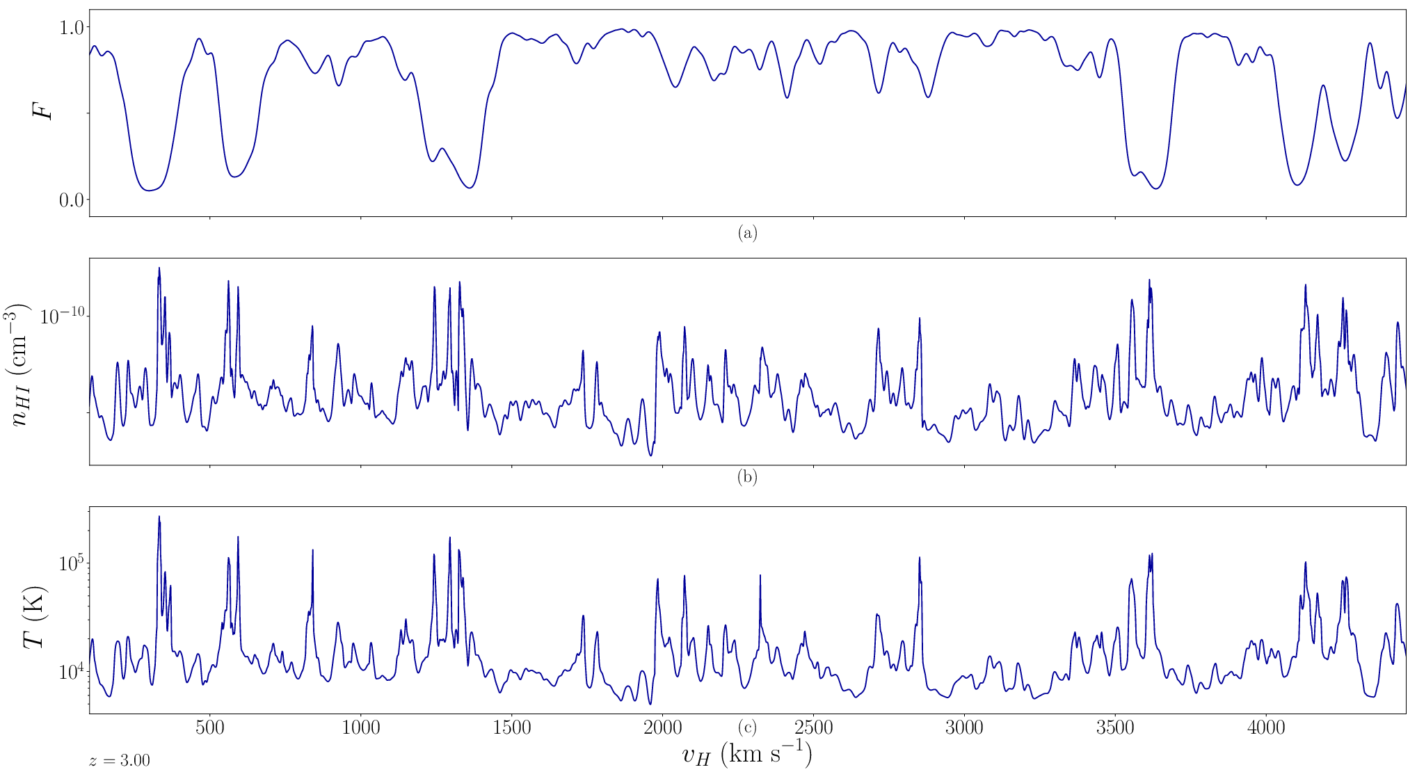
Figure 3 shows an example of a spectrum that passes through the center of our L-1024-40 simulation volume. In addition to the flux we also plot the number density of neutral hydrogen and temperature of the pixels along the LOS. We see that this figure serves as a consistency check in that when there is a trough in the transmitted flux, there is a peak in the optical depth, as expected. Additionally, the temperatures of the pixels fall mostly near , which is appropriate for the neutral hydrogen giving rise to the Ly forest (Becker et al. 2011, e.g.,).
Figure 4 illustrates a synthetic Ly forest spectrum through the center of the simulation volume for each of our dark energy models. These are offset from one another for visual clarity. All of the spectra, except for the DE2-40-1024 model, are quite similar to one another.

IV.2 Power Spectra
In order to calculate a power spectrum at each redshift, we bootstrapped a sample of eight-hundred synthetic Ly forest spectra from our pool. We chose eight-hundred spectra because it provided a large enough sample such that the distribution for the value of at each approached a normal distribution. The process described in Section III.3 was then applied to this bootstrapped sample in order to calculate one instance of the power spectrum.
The power spectra from our L-40-1024 simulation are shown along with observational data from Iršič et al. 2017; McDonald et al. 2006; McDonald et al. 2000 in Figure 5. Figure 5 shows that the shape of the simulated power spectra matches the observations quite well at all redshifts, but there appears to be a scaling issue that results in the simulated power spectra under-predicting the power at large (small scales) and low redshift ( and in particular). This result was also found by Bertone & White 2006 in their exploration of the effects of galactic winds on the Ly forest and in Peeples et al. 2010 in their exploration of the effects of thermal broadening and heating rates on the Ly forest. See Section V for a detailed discussion.

IV.2.1 Comparing Power Spectra
The goal of this project was to analyze possible signatures of time-dependent dark energy in the flux power spectrum of the Ly forest. To this end, we needed a statistical test that could quantify the differences between our calculated power spectra. We chose the k-sample Anderson-Darling (AD) test (Anderson & Darling 1952; Scholz & Stephens 1987) for this comparison. The AD statistic is based upon the distance between the distributions being compared (Scholz & Stephens 1987). We adopted the AD test for several reasons: first, it is distribution free44 4 Meaning that no underlying distribution needs to be specified; and second, when compared with the Kolmogorov-Smirnov (KS) test, the AD test puts more emphasis on the tails of the distribution, whereas the KS test emphasizes differences between distributions near the center. Since dark energy is a large-scale phenomenon, we expect most of the differences between power spectra, if they exist, to occur on the largest scales (smallest ), rather than in the central parts of the power spectrum; third, due to its increased sensitivity and ability to always be applied, the AD test has recently been recommended over the KS test in astronomy (Babu & Feigelson 2006, e.g.,).
| ADaa | C.V.aa | ADbb | C.V.bb | ADcc | C.V.cc | ADdd | C.V.dd | |
|---|---|---|---|---|---|---|---|---|
| 4.20 | -1.23 | 1.96 | -0.97 | 1.96 | -1.18 | 1.96 | -1.23 | 1.96 |
| 3.80 | -1.23 | 1.96 | -0.95 | 1.96 | -1.23 | 1.96 | -1.23 | 1.96 |
| 3.00 | -1.23 | 1.96 | -0.70 | 1.96 | -1.23 | 1.96 | -1.23 | 1.96 |
| 2.70 | -1.23 | 1.96 | -0.97 | 1.96 | -1.23 | 1.96 | -1.23 | 1.96 |
| 2.20 | -1.23 | 1.96 | -0.84 | 1.96 | -1.23 | 1.96 | -1.23 | 1.96 |
Note. — C.V. is the critical value of the AD statistic at the chosen significance level ().
When comparing power spectra, we chose the L-40-1024 simulation as our fiducial simulation to compare to our other simulations. This is because the cosmological constant is the de facto dark energy model in modern cosmology.
The results of our comparison are given in Table 3. We used scipy in order to conduct this test. The significance level of the test represents the probability of a Type I error (i.e., the probability of rejecting the null hypothesis of a statistical test given that the null hypothesis is true). The null hypothesis of the test is rejected if the value of the test statistic is larger than the value of the critical value for the given significance level. Table 3 shows that our AD statistics are lower than the critical values for in every case, indicating that one cannot reject the null hypothesis that the power spectra were drawn from the same distribution. This indicates that the intrinsic cosmic variance of the Ly forest power spectrum is in excess of the effects of time-dependent dark energy.

IV.3 Large-Scale Region of the Power Spectra
Since dark energy is a large-scale phenomenon, we expect any signatures of time-dependent dark energy to be most prominent at small . In order to investigate this, we zoomed in on each of the power spectra presented in fig. 6, as seen in fig. 7.

Figure 7 shows that there are indeed small deviations in the power spectra at large scales.
However, our synthetic power spectra were calculated from a pool of synthetic Ly forest spectra, which contain randomly chosen sight-lines through our simulation volumes. In order to investigate whether or not these deviations are real and not merely statistical variations, we re-ran our spectral extraction code with a fixed random number generator seed. This guarantees that the pool of synthetic Ly forest spectra for each simulation all contain identical sight-lines. The synthetic power spectra arising from these pools of identical sight-lines are given in fig. 8.

Figure 8 shows that nearly all of the deviations between the flux power spectra vanish when using a pool of identical sight-lines. This indicates that the variations shown in fig. 7 are mostly due to variations in the pool of spectra. However, fig. 8 retains the discrepancy in power between the DE2-40-1024 and the other four models. This indicates that the power spectrum is sensitive to time-dependent dark energy, even if the differences between observationally viable models are small.
IV.4 Resolution Study
Here we investigate the effects of resolution on our results. To this end we ran four additional simulations, the parameters of which are given in Table 4. These simulations cover several bases. The L-15-428 simulation has the same spatial resolution as our fiducial simulations, but with a smaller box size. The effects of this smaller box size are shown in Figure 9. We see that at larger scales the two power spectra are nearly identical, but at smaller scales, the L-15-428 simulation has an excess of power compared to the L-40-1024 simulation.
In addition to the L-15-428 simulation, we also have three other simulations, L-100-1024, L-25-428, and L-40-428, at varying spatial resolutions. These simulations are plotted alongside the fiducial L-40-1024 simulation in Figure 10. We see that at large scales each of the power spectra are nearly indistinguishable from one another. At smaller scales, however, there is a fairly substantial difference. The L-100-1024 simulation has under-predicted power whereas the L-25-428 simulation has over-predicted power as compared to the others. The L-40-428 and L-40-1024 simulations are nearly identical at all scales.
| Simulation Name | Number of DM Particles | Softening Length ( comoving) | Box Size ( comoving) | Particle Mass |
|---|---|---|---|---|
| L-100-1024 | ||||
| L-15-428 | ||||
| L-25-428 | ||||
| L-40-428 |


We compared each of our resolution study simulations to our fiducial L-40-1024 simulation using the AD test, just as we did for our main production simulations. The results of this test are given in table 5. The results indicate that, although there are visual differences between the power spectra a various resolutions, the statistical evidence is not strong enough to discriminate between the power spectra at the significance level, indicating that the effects of resolution do not affect our conclusions.
| ADaaL-100-1024 | C.V.aaL-100-1024 | ADbbL-15-428 | C.V.bbL-15-428 | ADccL-25-428 | C.V.ccL-25-428 | ADddL-40-428 | C.V.ddL-40-428 |
|---|---|---|---|---|---|---|---|
| -1.21 | 1.96 | -0.95 | 1.96 | -1.17 | 1.96 | -1.23 | 1.96 |
Note. — C.V. is the critical value of the AD statistic at the chosen significance level ().
V Discussion
This work has built upon the work performed in 89 in order to explore whether or not time-dependent dark energy leaves an observationally detectable signature in the flux power spectrum of the Ly forest. To this end, we extracted synthetic Ly forest spectra from high-resolution N-body simulations and used these to calculate the flux power spectrum. We used five different dark energy models, including the cosmological constant and four dynamical, parameterized dark energy models. These models were chosen from the posterior distributions as determined by Planck. In particular, of the four dynamical dark energy models we employed, three of them were chosen to lie at the fringes of this posterior, while the fourth was deliberately chosen to lie outside of the bounds determined by Planck to serve as an extreme example from which one might see a discernible effect on the power spectrum.
Bootstrapping from our pool of synthetic Ly forest spectra, we calculated a power spectrum for each dark energy model at each redshift. We then utilized the k-sample AD test in order to compare our power spectra arising from simulations with dynamical dark energy to the power spectrum from our simulation employing a cosmological constant. The AD test can always be applied and emphasizes the tails of the distributions where we expect the effects of dark energy to be most prominent (at small ). The results of these tests show that there is no statistically significant evidence to discriminate between the power spectra at the significance level.
This conclusion differs from the findings of 89, who determined that the dark energy models they employed could, in principle, be discriminated against using the optical depth power spectrum. It should be noted, however, that 89 used dark energy models that all had a constant EOS different from , whereas we have used dynamical models. Furthermore, the simulations employed by 89 were semi-analytic in nature whereas ours were N-body. In particular, we could determine that the statistical cosmic variance of the Ly forest power spectrum exceeds that of the signature of time-dependent dark energy. These two factors would seem to be consequential enough to account for our differences in conclusions.
There are several points that affect our analysis. First is the fact that, given our high resolution requirements, each of our simulations was strictly N-body out of consideration for the total run time. This necessitated that we calculate the hydrodynamic quantities (such as density and temperature) required for calculating a synthetic spectrum in post-processing. In particular, our temperature prescription is an empirically determined power law, which does not encapsulate all of the necessary physical processes going on in the IGM, such as self-shielding, radiative cooling, shocks due to stellar winds and supernovae, metal feedback, etc. These omissions may affect our temperature-density relation, which could have an impact on the small-scale power where the discrepancy between the calculated and observed power spectra was the greatest. In particular, Bertone & White 2006 showed that the effects of galactic winds on the small-scale power are non-trivial. However, since we are concerned with larger scales that are not as affected by baryonic physics and galactic winds, omission of these effects in our simulations should not affect our conclusions (see, however, Bolton et al. 2017 for the effects of these processes on the low-redshift flux power spectrum).
Further, Peeples et al. 2010 investigated the effect of various heating rates on the Ly forest and found that the thermal state of the IGM has a non-negligible effect on the Ly forest. In particular, their largest effect came from the inclusion of thermal broadening, which we also include. We note that these issues predominantly affect small-scale power, which we under predict. However, their effect on larger scales is not as significant, and so, while they could alter our power spectra, we do not expect the changes to be significant enough to affect our statistical conclusions.
A second aspect of our simulations that needs to be addressed is the box size. Since dark energy is a large-scale phenomenon, ideally one would like to have as large a box as possible in order to explore smaller modes. However, while larger scales would be probed by a larger simulation volume, the Ly forest is predominantly due to absorption near clusters and inside filaments. This makes the effects of Hubble broadening on the lines and the correlation between absorbers separated by voids a secondary effect, making it difficult to detect.
These points are highlighted in our resolution study. In every case, the effects of resolution on the power spectrum at large scales were negligible. While running in a larger box did probe larger scales, these scales are larger than those probed in the three observational datasets that we used in Figure 5. Our study showed that the effects of resolution are most prominent on small-scale power, with lower resolution simulations under-predicting the observed small-scale power. This is in keeping with the findings of other authors (McDonald 2003, e.g.,).
Interestingly, both of our simulations that were run in volumes of the same size (L-40-1024 and L-40-428) had very similar power spectra at all scales. This suggests that it is the box size, as opposed to the particle number, that has the largest resolution effect on the power spectrum.
As a caveat to our dark energy model selection, we must be aware that the distribution we were sampling from for our and values is a posterior distribution, wherein all of the other relevant cosmological parameters have been marginalized. However, given the computational complexity of our simulations, such a Bayesian approach utilizing Markov-Chain Monte-Carlo (MCMC) methods in order to perform a similar marginalization was not feasible.
Ideally, one would like to run a large grid of simulations from which MCMC analysis could be used to perform the same marginalization over the cosmological parameters, as was done in Planck Collaboration et al. 2015. While such a Bayesian approach would allow us to find the maximally likely contours when comparing simulation to observational data, our goal was to explore whether or not signatures from dark energy manifested themselves in the power spectrum at a large enough level to be distinguished from the cosmic variance as opposed to trying to find the best-fit dark energy model. This makes an MCMC approach of limited usefulness with regards to investigating the effects of time-dependent dark energy on the Ly forest.
Finally, we note that the fact remains that the effects of dark energy on the Ly forest are sub-dominant to those of baryonic physics in the IGM. This implies that, whether performing a full marginalization over the cosmological parameters or not, the power spectra arising from varying time-dependent dark energy models will be extremely similar to one another. Our analysis shows that such models cannot be statistically discriminated against due to cosmic variance even at the level of idealized simulations where we are in possession of full knowledge of the physical situation. This means that any attempt to search for a dark energy signal in the observed flux power spectrum of the Ly forest, where the uncertainties are far larger, is, and likely will remain, challenging.
References
- Abbott et al. (2016) Abbott, T., Abdalla, F. B., Allam, S., et al. 2016, Phys. Rev. D, 94, 022001
- Amendola & Tsujikawa (2010) Amendola, L., & Tsujikawa, S. 2010, Dark Energy: Theory and Observations
- Anderson & Darling (1952) Anderson, T. W., & Darling, D. A. 1952, Ann. Math. Statist., 23, 193. https://doi.org/10.1214/aoms/1177729437
- Armendáriz-Picón et al. (2000) Armendáriz-Picón, C., Mukhanov, V., & Steinhardt, P. J. 2000, Physical Review Letters, 85, 4438
- Babu & Feigelson (2006) Babu, G. J., & Feigelson, E. D. 2006, in Astronomical Society of the Pacific Conference Series, Vol. 351, Astronomical Data Analysis Software and Systems XV, ed. C. Gabriel, C. Arviset, D. Ponz, & S. Enrique, 127
- Becker et al. (2011) Becker, G. D., Bolton, J. S., Haehnelt, M. G., & Sargent, W. L. W. 2011, MNRAS, 410, 1096
- Bertone (2003) Bertone, S. 2003, PhD thesis, Università degli Studi di Torino
- Bertone & White (2006) Bertone, S., & White, S. D. M. 2006, MNRAS, 367, 247
- Bi et al. (1995) Bi, H., Ge, J., & Fang, L.-Z. 1995, ApJ, 452, 90
- Biswas et al. (2010) Biswas, R., Alizadeh, E., & Wandelt, B. D. 2010, Phys. Rev. D, 82, 023002
- Blake et al. (2011) Blake, C., Davis, T., Poole, G. B., et al. 2011, MNRAS, 415, 2892
- Bolton et al. (2017) Bolton, J. S., Puchwein, E., Sijacki, D., et al. 2017, MNRAS, 464, 897
- Bond et al. (1996) Bond, J. R., Kofman, L., & Pogosyan, D. 1996, Nature, 380, 603
- Bordoloi et al. (2014) Bordoloi, R., Tumlinson, J., Werk, J. K., et al. 2014, ApJ, 796, 136
- Bos et al. (2012) Bos, E. G. P., van de Weygaert, R., Dolag, K., & Pettorino, V. 2012, MNRAS, 426, 440
- Brook et al. (2014) Brook, C. B., Di Cintio, A., Knebe, A., et al. 2014, ApJ, 784, L14
- Caldwell et al. (1998) Caldwell, R. R., Dave, R., & Steinhardt, P. J. 1998, Physical Review Letters, 80, 1582
- Carroll et al. (2005) Carroll, S. M., de Felice, A., Duvvuri, V., et al. 2005, Phys. Rev. D, 71, 063513
- Célérier (2000) Célérier, M.-N. 2000, A&A, 353, 63
- Cen et al. (1994) Cen, R., Miralda-Escudé, J., Ostriker, J. P., & Rauch, M. 1994, ApJ, 437, L9
- Chevallier & Polarski (2001) Chevallier, M., & Polarski, D. 2001, International Journal of Modern Physics D, 10, 213
- Cole et al. (2005) Cole, S., Percival, W. J., Peacock, J. A., et al. 2005, MNRAS, 362, 505
- Corasaniti & Copeland (2003) Corasaniti, P. S., & Copeland, E. J. 2003, Phys. Rev. D, 67, 063521
- Croton (2013) Croton, D. J. 2013, PASA, 30, 52
- de Jong et al. (2013) de Jong, J. T. A., Verdoes Kleijn, G. A., Kuijken, K. H., & Valentijn, E. A. 2013, Experimental Astronomy, 35, 25. https://doi.org/10.1007/s10686-012-9306-1
- Dehnen & Aly (2012) Dehnen, W., & Aly, H. 2012, MNRAS, 425, 1068
- Dolag et al. (2004) Dolag, K., Bartelmann, M., Perrotta, F., et al. 2004, A&A, 416, 853
- Duffy et al. (2012) Duffy, A. R., Kay, S. T., Battye, R. A., et al. 2012, MNRAS, 420, 2799
- Dupé et al. (2011) Dupé, F.-X., Rassat, A., Starck, J.-L., & Fadili, M. J. 2011, A&A, 534, A51
- Eisenstein et al. (2005) Eisenstein, D. J., Zehavi, I., Hogg, D. W., et al. 2005, ApJ, 633, 560
- Enqvist (2008) Enqvist, K. 2008, General Relativity and Gravitation, 40, 451
- Garcia-Fernandez et al. (2016) Garcia-Fernandez, M., Sánchez, E., Sevilla-Noarbe, I., et al. 2016, ArXiv e-prints, arXiv:1611.10326
- Garnavich et al. (1998) Garnavich, P. M., Jha, S., Challis, P., et al. 1998, ApJ, 509, 74
- Gerhard & Spergel (1992) Gerhard, O. E., & Spergel, D. N. 1992, ApJ, 389, L9
- Gerke & Efstathiou (2002) Gerke, B. F., & Efstathiou, G. 2002, MNRAS, 335, 33
- Giannantonio et al. (2008) Giannantonio, T., Scranton, R., Crittenden, R. G., et al. 2008, Phys. Rev. D, 77, 123520
- Gill et al. (2004) Gill, S. P. D., Knebe, A., & Gibson, B. K. 2004, MNRAS, 351, 399
- Greig (2013) Greig, B. 2013, PhD thesis, University of Melbourne
- Haardt & Madau (1996) Haardt, F., & Madau, P. 1996, ApJ, 461, 20
- Haardt & Madau (2012) —. 2012, ApJ, 746, 125
- Ho et al. (2008) Ho, S., Hirata, C., Padmanabhan, N., Seljak, U., & Bahcall, N. 2008, Phys. Rev. D, 78, 043519
- Hui et al. (2001) Hui, L., Burles, S., Seljak, U., et al. 2001, ApJ, 552, 15
- Hui & Gnedin (1997) Hui, L., & Gnedin, N. Y. 1997, MNRAS, 292, 27
- Hummels et al. (2016) Hummels, C., Smith, B., & Silvia, D. 2016, ArXiv e-prints, arXiv:1612.03935
- Iguchi et al. (2002) Iguchi, H., Nakamura, T., & Nakao, K. 2002, Progress of Theoretical Physics, 108, 809
- Iršič & Viel (2014) Iršič, V., & Viel, M. 2014, J. Cosmology Astropart. Phys, 12, 024
- Iršič et al. (2017) Iršič, V., Viel, M., Berg, T. A. M., et al. 2017, MNRAS, 466, 4332
- Joyce et al. (2016) Joyce, A., Lombriser, L., & Schmidt, F. 2016, Annual Review of Nuclear and Particle Science, 66, 95
- Kim et al. (2002) Kim, T.-S., Carswell, R. F., Cristiani, S., D’Odorico, S., & Giallongo, E. 2002, MNRAS, 335, 555
- Knollmann & Knebe (2009) Knollmann, S. R., & Knebe, A. 2009, ApJS, 182, 608
- Komatsu et al. (2011) Komatsu, E., Smith, K. M., Dunkley, J., et al. 2011, ApJS, 192, 18
- Kujat et al. (2002) Kujat, J., Linn, A. M., Scherrer, R. J., & Weinberg, D. H. 2002, ApJ, 572, 1
- Lavaux & Wandelt (2010) Lavaux, G., & Wandelt, B. D. 2010, MNRAS, 403, 1392
- Lavaux & Wandelt (2012) —. 2012, ApJ, 754, 109
- Lee & Park (2009) Lee, J., & Park, D. 2009, ApJ, 696, L10
- Linder (2003) Linder, E. V. 2003, Physical Review Letters, 90, 091301
- Lue et al. (2004) Lue, A., Scoccimarro, R., & Starkman, G. 2004, Phys. Rev. D, 69, 044005
- Madau et al. (1999) Madau, P., Haardt, F., & Rees, M. J. 1999, ApJ, 514, 648
- McDonald (2003) McDonald, P. 2003, ApJ, 585, 34
- McDonald et al. (2000) McDonald, P., Miralda-Escudé, J., Rauch, M., et al. 2000, ApJ, 543, 1
- McDonald et al. (2006) McDonald, P., Seljak, U., Burles, S., et al. 2006, ApJS, 163, 80
- McQuinn (2016) McQuinn, M. 2016, ARA&A, 54, 313
- Meiksin & White (2001) Meiksin, A., & White, M. 2001, MNRAS, 324, 141
- Mo & White (2002) Mo, H. J., & White, S. D. M. 2002, MNRAS, 336, 112
- Ostriker & Steinhardt (1995) Ostriker, J. P., & Steinhardt, P. J. 1995, Nature, 377, 600
- Park & Lee (2007) Park, D., & Lee, J. 2007, Physical Review Letters, 98, 081301
- Peeples et al. (2010) Peeples, M. S., Weinberg, D. H., Davé, R., Fardal, M. A., & Katz, N. 2010, MNRAS, 404, 1281
- Perlmutter et al. (1999) Perlmutter, S., Aldering, G., Goldhaber, G., et al. 1999, ApJ, 517, 565
- Planck Collaboration et al. (2014) Planck Collaboration, Ade, P. A. R., Aghanim, N., et al. 2014, A&A, 571, A16
- Planck Collaboration et al. (2015) —. 2015, ArXiv e-prints, arXiv:1502.01590
- Planck Collaboration et al. (2016) —. 2016, A&A, 594, A13
- Planck Collaboration et al. (2018) Planck Collaboration, Aghanim, N., Akrami, Y., et al. 2018, ArXiv e-prints, arXiv:1807.06209
- Popping et al. (2009) Popping, A., Davé, R., Braun, R., & Oppenheimer, B. D. 2009, A&A, 504, 15
- Rauch (1998) Rauch, M. 1998, ARA&A, 36, 267
- Riess et al. (1998) Riess, A. G., Filippenko, A. V., Challis, P., et al. 1998, AJ, 116, 1009
- Rivera-Thorsen et al. (2017) Rivera-Thorsen, T. E., Dahle, H., Gronke, M., et al. 2017, A&A, 608, L4
- Schaye & Dalla Vecchia (2008) Schaye, J., & Dalla Vecchia, C. 2008, MNRAS, 383, 1210
- Scholz & Stephens (1987) Scholz, F. W., & Stephens, M. A. 1987, Journal of the American Statistical Association, 82, 918. https://doi.org/10.1080/01621459.1987.10478517
- Schrabback et al. (2010) Schrabback, T., Hartlap, J., Joachimi, B., et al. 2010, A&A, 516, A63
- Scoccimarro et al. (2012) Scoccimarro, R., Hui, L., Manera, M., & Chan, K. C. 2012, Phys. Rev. D, 85, 083002
- Shoji & Lee (2012) Shoji, M., & Lee, J. 2012, ArXiv e-prints, arXiv:1203.0869
- Snedden et al. (2016) Snedden, A., Coughlin, J., Phillips, L. A., Mathews, G., & Suh, I.-S. 2016, MNRAS, 455, 2804
- Spergel et al. (2003) Spergel, D. N., Verde, L., Peiris, H. V., et al. 2003, ApJS, 148, 175
- Springel (2005) Springel, V. 2005, MNRAS, 364, 1105
- Theuns et al. (1998) Theuns, T., Leonard, A., Efstathiou, G., Pearce, F. R., & Thomas, P. A. 1998, MNRAS, 301, 478
- Tomita (2000) Tomita, K. 2000, ApJ, 529, 38
- Tomita (2001) —. 2001, MNRAS, 326, 287
- Vanzella et al. (2018) Vanzella, E., Nonino, M., Cupani, G., et al. 2018, MNRAS, 476, L15
- Viel et al. (2003) Viel, M., Matarrese, S., Theuns, T., Munshi, D., & Wang, Y. 2003, MNRAS, 340, L47
- Zhao & Mathews (2011) Zhao, X., & Mathews, G. J. 2011, Phys. Rev. D, 83, 023524