跳到论文正文
W Papers独立论文阅读器 arXiv:1812.03108 论文正文 计算阅读时间 · 0%
引用这篇论文根据当前论文元数据生成,正式投稿前建议核对。


License: arXiv.org perpetual non-exclusive license
arXiv:1812.03108v1 [math.ST] 07 Dec 2018

Principal components analysis of regularly varying functions

Piotr Kokoszka
Colorado State University
   Stilian Stoev
University of Michigan
   Qian Xiong
Colorado State University

The paper is concerned with asymptotic properties of the principal components analysis of functional data. The currently available results assume the existence of the fourth moment. We develop analogous results in a setting which does not require this assumption. Instead, we assume that the observed functions are regularly varying. We derive the asymptotic distribution of the sample covariance operator and of the sample functional principal components. We obtain a number of results on the convergence of moments and almost sure convergence. We apply the new theory to establish the consistency of the regression operator in a functional linear model.

Key words: Functional data, Principal components, Regular variation

1 Introduction

A fundamental technique of functional data analysis is to replace infinite dimensional curves by coefficients of their projections onto suitable, fixed or data–driven, systems, e.g. [bosq:2000], [ramsay:silverman:2005], [HKbook], [hsing:eubank:2015]. A finite number of these coefficients encode the shape of the curves and are amenable to various statistical procedures. The best systems are those that lead to low dimensional representations, and so provide the most efficient dimension reduction. Of these, the functional principal components (FPCs) have been most extensively used, with hundreds of papers dedicated to the various aspects of their theory and applications.

If X,X1,X2,…,XNX,X_{1},X_{2},\ldots,X_{N} are mean zero iid functions in L2L^{2} with E​‖X‖2<∞E\left\|X\right\|^{2}<\infty, then

Xn​(t)=∑j=1∞ξn​j​vj​(t),E​ξn​j2=λj.X_{n}(t)=\sum_{j=1}^{\infty}\xi_{nj}v_{j}(t),\ \ \ E\xi_{nj}^{2}=\lambda_{j}. (1.1)

The FPCs vjv_{j} and the eigenvalues λj\lambda_{j} are, respectively, the eigenfunctions and the eigenvalues of the covariance operator C:L2→L2C:L^{2}\to L^{2} defined by C⁡(x)​(t)=∫Cov​(X⁡(t),X⁡(s))​x​(s)​𝑑sC(x)(t)=\int\hbox{\rm Cov}(X(t),X(s))x(s)ds As such, the vjv_{j} are orthogonal. We assume they are normalized to unit norm. The vjv_{j} form an optimal orthonormal basis for dimension reduction measured by the L2L^{2} norm, see e.g. Theorem 11.4.1 in [KRbook].

The vjv_{j} and the λj\lambda_{j} are estimated by v^j\hat{v}_{j} and λ^j\hat{\lambda}_{j} defined by

∫c^​(t,s)​v^j​(s)​𝑑s=λ^j​v^j​(t),\int\hat{c}(t,s)\hat{v}_{j}(s)ds=\hat{\lambda}_{j}\hat{v}_{j}(t), (1.2)

where

c^​(t,s)=1N​∑n=1NXn​(t)​Xn​(s).\hat{c}(t,s)=\frac{1}{N}\sum_{n=1}^{N}X_{n}(t)X_{n}(s). (1.3)

Like the vjv_{j}, the v^j\hat{v}_{j} are defined only up to a sign. Thus, strictly speaking, in the formulas that follow, the v^j\hat{v}_{j} would need to be replaced with c^j​v^j\hat{c}_{j}\hat{v}_{j}, where c^j=sign⁡⟨v^j,vj⟩\hat{c}_{j}={\rm sign}\left\langle\hat{v}_{j},v_{j}\right\rangle. As is customary, to lighten the notation, we assume that the orientations of vjv_{j} and v^j\hat{v}_{j} match, i.e. c^j=1\hat{c}_{j}=1.

Under the existence of the fourth moment,

E​‖X‖4={∫X2​(t)​𝑑t}2<∞,E\left\|X\right\|^{4}=\left\{\int X^{2}(t)dt\right\}^{2}<\infty, (1.4)

and assuming λ1>λ2>…\lambda_{1}>\lambda_{2}>\ldots, it has been shown that for each j≥1j\geq 1,

lim supN→∞N​E​‖v^j−vj‖2<∞,lim supN→∞N​E​(λ^j−λj)2<∞,\limsup_{N\to\infty}NE\left\|\hat{v}_{j}-v_{j}\right\|^{2}<\infty,\ \ \ \limsup_{N\to\infty}NE\left(\hat{\lambda}_{j}-\lambda_{j}\right)^{2}<\infty, (1.5)
N1/2​(λ^j−λj)→dN⁡(0,σj2),N^{1/2}(\hat{\lambda}_{j}-\lambda_{j})\stackrel{{\scriptstyle\mbox{$\scriptstyle d$}}}{{\rightarrow}}N(0,\sigma_{j}^{2}), (1.6)
N1/2​(v^j−vj)→dN⁡(0,Cj),N^{1/2}(\hat{v}_{j}-v_{j})\stackrel{{\scriptstyle\mbox{$\scriptstyle d$}}}{{\rightarrow}}N(0,C_{j}), (1.7)

for a suitably defined variance σj2\sigma_{j}^{2} and a covariance operator CjC_{j}. The above relations, especially (1.5), have been used to derive large sample justifications of inferential procedures based on the estimated FPCs v^j\hat{v}_{j}. In most scenarios, one can show that replacing the v^j\hat{v}_{j} by the vjv_{j} and the λ^j\hat{\lambda}_{j} by the λj\lambda_{j} is asymptotically negligible. Relations (1.5) were established by [dauxois:1982] and extended to weakly dependent functional time series by [hormann:kokoszka:2010]. Relations (1.6) and (1.7) follow from the results of [kokoszka:reimherr:2013]. In case of continuous functions satisfying regularity conditions, they follow from the results of [hall:h-n:2006].

A crucial assumption for the relations (1.5)–(1.7) to hold is the existence of the fourth moment, i.e. (1.4), the iid assumption can be relaxed in many ways. Nothing is at present known about the asymptotic properties of the FPCs and their eigenvalues if (1.4) does not hold. Our objective is to explore what can be said about the asymptotic behavior of C^\widehat{C}, v^j\hat{v}_{j} and λ^j\hat{\lambda}_{j} if (1.4) fails. We would thus like to consider the case of E​‖Xn‖2<∞E\|X_{n}\|^{2}<\infty and E​‖Xn‖4=∞E\|X_{n}\|^{4}=\infty. Such an assumption is however too general. From mid 1980s to mid 1990s similar questions were posed for scalar time series for which the fourth or even second moment does not exist. A number of results pertaining to the convergence of sample covariances and the periodogram have been derived under the assumption of regularly varying tails, e.g. Davis and Resnick (?, ?), [kluppelberg:mikosch:1994], [mikosch:gka:1995], [kokoszka:taqqu:1996], [anderson:meerschaert:1997]; many others are summarized in the monograph of [embrechts:kluppelberg:mikosch:1997]. The assumption of regular variation is natural because non–normal stable limits can be derived by establishing a connection to random variables in a stable domain of attraction, which is characterized by regular variation. This is the approach we take. We assume that the functions XnX_{n} are regularly varying in the space L2L^{2} with the index α∈(2,4)\alpha\in(2,4), which implies E​‖Xn‖2<∞E\|X_{n}\|^{2}<\infty and E​‖Xn‖4=∞E\|X_{n}\|^{4}=\infty. Suitable definitions and assumptions are presented in Section 2.

The paper is organized as follows. The remainder of the introduction provides a practical motivation for the theory we develop. It is not necessary to understand the contribution of the paper, but, we think, it gives a good feel for what is being studied. The formal exposition begins in Section 2, in which notation and assumptions are specified. Section 3 is dedicated to the convergence of the sample covariance operator (the integral operator with kernel (1.3)). These results are then used in Section 4 to derive various convergence results for the sample FPCs and their eigenvalues. Section 5 shows how the results derived in previous sections can be used in a context of a functional regression model. Its objective is to illustrate the applicability of our theory in a well–known and extensively studied setting. It is hoped that it will motivate and guide applications to other problems of functional data analysis. All proofs which go beyond simple arguments are presented in Online material.
Refer to caption
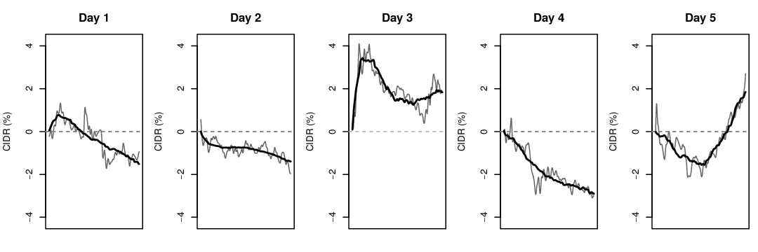
Figure 1: Five consecutive intraday return curves, Walmart stock. The raw returns are noisy grey lines. The smoother black lines are approximations X^i​(t)=∑j=13ξ^i​j​v^j\widehat{X}_{i}(t)=\sum_{j=1}^{3}\hat{\xi}_{ij}\hat{v}_{j}.

We conclude this introduction by presenting a specific data context. Denote by Pi​(t)P_{i}(t) the price of an asset at time tt of trading day ii. For the assets we consider in our illustration, tt is time in minutes between 9:30 and and 16:00 EST (NYSE opening times) rescaled to the unit interval (0,1)(0,1). The intraday return curve on day ii is defined by Xi​(t)=log⁡Pi​(t)−log⁡Pi​(0)X_{i}(t)=\log P_{i}(t)-\log P_{i}(0). In practice, Pi​(0)P_{i}(0) is the price after the first minute of trading. The curves XiX_{i} show how the return accumulates over the trading day, see e.g. [lucca:moench:2015]; examples of are shown in Figure 1.

Refer to caption
Figure 2: The first three sample FPCs of intraday returns on Walmart stock.

The first three sample FPCs, v^1,v^2,v^3\hat{v}_{1},\hat{v}_{2},\hat{v}_{3}, are shown in Figure 2. They are computed, using (1.2), from minute-by-minute Walmart returns form July 05, 2006 to Dec 30, 2011, N=1,378N=1,378 trading days. (This time interval is used for the other assets we consider.) The curves X^i=∑j=13ξ^i​j​v^j\widehat{X}_{i}=\sum_{j=1}^{3}\hat{\xi}_{ij}\hat{v}_{j}, with the scores ξ^i​j=∫Xi​(t)​v^j​(t)​𝑑t\hat{\xi}_{ij}=\int X_{i}(t)\hat{v}_{j}(t)dt, visually approximate the curves XiX_{i} well. One can thus expect that the v^j\hat{v}_{j} (with properly adjusted sign) are good estimators of the population FPCs vjv_{j} in (1.1). Relations (1.5) and (1.7) show that this is indeed the case, if E​‖X‖4<∞E\|X\|^{4}<\infty. (The curves XiX_{i} can be assumed to form a stationary time series in L2L^{2}, see [horvath:kokoszka:rice:2014].) We will now argue that the assumption of the finite fourth moment is not realistic, so, with the currently available theory, it is not clear if the v^j\hat{v}_{j} are good estimators of the vjv_{j}. If E​‖X‖4<∞E\|X\|^{4}<\infty, then E​ξ1​j4<∞E\xi_{1j}^{4}<\infty for every jj. Figure 3 shows the Hill plots of the sample score ξ^i​j\hat{\xi}_{ij} for two stocks and for j=1,2,3j=1,2,3. Hill plots for other blue chip stocks look similar. These plots illustrate several properties. 1) It is reasonable to assume that the scores have Pareto tails. 2) The tail index α\alpha is smaller than 4, implying that the fourth moment does not exist. 3) It is reasonable to assume that the tail index does not depend on jj and is between 2 and 4. With such a motivation, we are now able to formalize in the next section the setting of this paper.

Refer to caption
Figure 3: Hill plots (an estimate of α\alpha as a function of upper order statistics) for sample FPC scores for Walmart (left) and IBM (right). From top to bottom: levels j=1,2,3j=1,2,3.

2 Preliminaries

The functions XnX_{n} are assumed to be independent and identically distributed in L2L^{2}, with the same distribution as XX, which is regularly varying with index α∈(2,4)\alpha\in(2,4). By L2:=L2​(𝒯)L^{2}:=L^{2}({\mathcal{T}}), we denote the usual separable Hilbert space of square integrable functions on some compact subset 𝒯{\mathcal{T}} of an Euclidean space. In a typical FDA framework, 𝒯=[0,1]{\mathcal{T}}=[0,1], e.g. Chapter 2 of [HKbook]. Regular variation in finite–dimensional spaces has been a topic of extensive research for decades, see e.g. Resnick (?, ?) and [meerschaert:scheffler:2001book]. We shall need the concept of regular variation of measures on infinitely-dimensional function spaces. To this end, we start by recalling some terminology and fundamental facts about regularly varying functions.

A measurable function L:(0,∞)→ℝL:(0,\infty)\to\mathbb{R} is said to be slowly varying (at infinity) if, for all λ>0\lambda>0,

L⁡(λ​u)L⁡(u)→1, as ​u→∞.\frac{L(\lambda u)}{L(u)}\to 1,\ \quad\mbox{ as }u\to\infty.

Functions of the form R⁡(u)=uρ​L​(u)R(u)=u^{\rho}L(u) are said to be regularly varying with exponent ρ∈ℝ\rho\in{\mathbb{R}}.

The notion of regular variation extends to measures and provides an elegant and powerful framework for establishing limit theorems. It was first introduced by [meerschaert:1984] and has been since extended to Banach and even metric spaces using the notion of M0M_{0} convergence (see e.g. [hult:lindskog:2006]). Even though we will work only with Hilbert spaces, we review the theory in a more general context.

Consider a separable Banach space 𝔹\mathbb{B} and let Bϵ:={z∈𝔹:‖z‖<ϵ}B_{\epsilon}:=\{z\in\mathbb{B}\,:\,\|z\|<\epsilon\} be the open ball of radius ϵ>0\epsilon>0, centered at the origin. A Borel measure μ\mu defined on 𝔹0:=𝔹\{𝟎}\mathbb{B}_{0}:=\mathbb{B}\backslash\{\mathbf{0}\} is said to be boundedly finite if μ⁡(A)<∞\mu(A)<\infty, for all Borel sets that are bounded away from 𝟎\mathbf{0}, that is, such that A∩Bϵ=∅A\cap B_{\epsilon}=\emptyset, for some ϵ>0\epsilon>0. Let 𝕄0\mathbb{M}_{0} be the collection of all such measures. For μn,μ∈𝕄0\mu_{n},\mu\in\mathbb{M}_{0}, we say that the μn\mu_{n} converge to μ\mu in the M0M_{0} topology, if μn​(A)→μ​(A)\mu_{n}(A)\to\mu(A), for all bounded away from 𝟎\mathbf{0}, μ\mu-continuity Borel sets AA, i.e., such that μ⁡(∂A)=0\mu(\partial A)=0, where ∂A:=A¯∖A∘\partial A:=\overline{A}\setminus A^{\circ} denotes the boundary of AA. The M0M_{0} convergence can be metrized such that 𝕄0\mathbb{M}_{0} becomes a complete separable metric space (Theorem 2.3 in [hult:lindskog:2006] and also Section 2.2. of [meinguet:2010]). The following result is known, see e.g. Chapter 2 of [meinguet:2010] and references therein.

Proposition 2.1

Let XX be a random element in a separable Banach space 𝔹\mathbb{B} and α>0\alpha>0. The following three statements are equivalent:

  • (i)

    For some slowly varying function LL,

    P⁡(‖X‖>u)=u−α​L​(u)P(\left\|X\right\|>u)=u^{-\alpha}L(u) (2.1)

    and

    P(u−1X∈⋅)P⁡(‖X‖>u)⟶M0μ⁡(⋅),u→∞,\frac{P(u^{-1}X\in\cdot)}{P(\left\|X\right\|>u)}\stackrel{{\scriptstyle M_{0}}}{{\longrightarrow}}\mu(\cdot),\ \ u\to\infty, (2.2)

    where μ\mu is a non-null measure on the Borel σ\sigma-field ℬ⁡(𝔹0)\mathcal{B}(\mathbb{B}_{0}) of 𝔹0=𝔹\{𝟎}\mathbb{B}_{0}=\mathbb{B}\backslash\left\{\mathbf{0}\right\}.

  • (ii)

    There exists a probability measure Γ\Gamma on the unit sphere 𝕊\mathbb{S} in 𝔹\mathbb{B} such that, for every t>0t>0,

    P(‖X‖>tu,X/‖X‖∈⋅)P⁡(‖X‖>u)⟶wt−α​Γ​(⋅),u→∞.\frac{P(\left\|X\right\|>tu,X/\left\|X\right\|\in\cdot)}{P(\left\|X\right\|>u)}\stackrel{{\scriptstyle w}}{{\longrightarrow}}t^{-\alpha}\Gamma(\cdot),\ \ u\to\infty.
  • (iii)

    Relation (2.1) holds, and for the same spectral measure Γ\Gamma in (ii),

    P(X/‖X‖∈⋅|‖X‖>u)⟶wΓ(⋅),u→∞.P\left(X/\left\|X\right\|\in\cdot|\left\|X\right\|>u\right)\stackrel{{\scriptstyle w}}{{\longrightarrow}}\Gamma(\cdot),\ \ u\to\infty.
Definition 2.1.

If any one of the equivalent conditions in Proposition 2.1 hold, we shall say that XX is regularly varying with index α\alpha. The measures μ\mu and Γ\Gamma will be referred to as exponent and angular measures of XX, respectively.

The measure Γ\Gamma is sometimes called the spectral measure, but we will use the adjective “spectral” in the context of stable measures which appear in Section 3. It is important to distinguish the angular measure of a regularly varying random function and a spectral measure of a stable distribution, although they are related. We also note that we call α\alpha the tail index, and −α-\alpha the tail exponent.

We will work under the following assumption.

Assumption 2.1

The random element XX in the separable Hilbert space H=L2H=L^{2} has mean zero and is regularly varying with index α∈(2,4)\alpha\in(2,4). The observations X1,X2,…X_{1},X_{2},\ldots are independent copies of XX.

Assumption 2.1 is a coordinate free condition not related in any way to functional principal components. The next assumption relates the asymptotic behavior of the FPC scores to the assumed regular variation. It implies, in particular, that the expansion X⁡(t)=∑j=1∞ξj​vj​(t)X(t)=\sum_{j=1}^{\infty}\xi_{j}v_{j}(t) contains infinitely many terms, so that we study infinite dimensional objects. We will see in the proofs of Proposition 3.3 and Theorem 3.6 that under Assumption 2.1 the limit

Qn​m=limu→∞P⁡({∑j=n∞ξj2}1/2​{∑j=m∞ξj2}1/2>u)P⁡(∑j=1∞ξj2>u)Q_{nm}=\lim_{u\to\infty}\frac{P\left(\left\{\sum_{j=n}^{\infty}\xi_{j}^{2}\right\}^{1/2}\left\{\sum_{j=m}^{\infty}\xi_{j}^{2}\right\}^{1/2}>u\right)}{P\left(\sum_{j=1}^{\infty}\xi_{j}^{2}>u\right)}

exists and is finite. We impose the following assumption related to condition (2.2).

Assumption 2.2

For every n,m≥1n,m\geq 1, Qn​m>0Q_{nm}>0.

Assumption 2.2 postulates, intuitively, that the tail sums ∑j=n∞ξj2\sum_{j=n}^{\infty}\xi_{j}^{2} must have extreme probability tails comparable to that of ‖X‖2\|X\|^{2}.

We now collect several useful facts that will be used in the following. The exponent measure μ\mu satisfies

μ⁡(t​A)=t−α​μ​(A),∀t>0,A∈ℬ⁡(𝔹0).\mu(tA)=t^{-\alpha}\mu(A),\ \ \forall t>0,\ \ A\in\mathcal{B}(\mathbb{B}_{0}). (2.3)

It admits the polar coordinate representation via the angular measure Γ\Gamma. That is, if x=r​θx=r\theta, where r:=‖x‖r:=\|x\| and θ=x/‖x‖,\theta=x/\|x\|, for x≠𝟎x\not=\mathbf{0}, we have

μ⁡(d​x)=α​r−α−1​d​r​Γ​(d​θ).\mu(dx)=\alpha r^{-\alpha-1}dr\Gamma(d\theta). (2.4)

This means that for every bounded measurable function ff that vanishes on a neighborhood of 𝟎\mathbf{0}, we have

∫𝔹f⁡(x)​μ​(𝑑x)=∫𝕊∫0∞f⁡(r​θ)​α​r−α−1​𝑑r​Γ​(𝑑θ).\int_{\mathbb{B}}f(x)\mu(dx)=\int_{\mathbb{S}}\int_{0}^{\infty}f(r\theta)\alpha r^{-\alpha-1}dr\Gamma(d\theta).

There exists a sequence {aN}\left\{a_{N}\right\} such that

N​P​(X∈aN​A)→μ⁡(A),NP\left(X\in a_{N}A\right)\to\mu(A), (2.5)

for any set AA in ℬ⁡(𝔹0)\mathcal{B}(\mathbb{B}_{0}) with μ⁡(∂A)=0\mu(\partial A)=0. One can take, for example,

aN=N1/α​L0​(N),a_{N}=N^{1/\alpha}L_{0}(N), (2.6)

with a slowly varying function L0L_{0} satisfying L0−α​(N)​L​(N1/α​L0​(N))→1L_{0}^{-\alpha}(N)L(N^{1/\alpha}L_{0}(N))\to 1.

We will work with Hilbert–Schmidt operators. A linear operator Ψ:H→H\Psi:H\to H is Hilbert–Schmidt if ∑j=1∞‖Ψ⁡(ej)‖2<∞\sum_{j=1}^{\infty}\left\|\Psi(e_{j})\right\|^{2}<\infty, where {ej}\left\{e_{j}\right\} is any orthonormal basis of HH. Every Hilbert–Schmidt operator is bounded. The space of Hilbert–Schmidt operators will be denoted by 𝒮{\mathcal{S}}. It is itself a separable Hilbert space with the inner product

⟨Ψ1,Ψ2⟩𝒮=∑j=1∞⟨Ψ1​(ej),Ψ2​(ej)⟩.\left\langle\Psi_{1},\Psi_{2}\right\rangle_{\mathcal{S}}=\sum_{j=1}^{\infty}\left\langle\Psi_{1}(e_{j}),\Psi_{2}(e_{j})\right\rangle.

If Ψ\Psi is an integral operator defined by Ψ⁡(x)​(t)=∫ψ⁡(t,s)​x​(s)​𝑑s,x∈L2\Psi(x)(t)=\int\psi(t,s)x(s)ds,\ x\in L^{2}, then ‖Ψ‖𝒮2=∬ψ2​(t,s)​𝑑t​𝑑s\|\Psi\|_{{\mathcal{S}}}^{2}=\iint\psi^{2}(t,s)dtds.

Relations (1.5) essentially follow from the bound

E​‖C^−C‖𝒮2≤N−1​E​‖X‖4,E\left\|\widehat{C}-C\right\|_{{\mathcal{S}}}^{2}\leq N^{-1}E\left\|X\right\|^{4},

where the subscript 𝒮{\mathcal{S}} indicates the Hilbert–Schmidt norm. Under Assumption 2.1 such a bound is useless because, by (2.1), E​‖X‖4=∞E\left\|X\right\|^{4}=\infty. In fact, one can show that under Assumption 2.1, E​‖C^‖𝒮2=∞E\|\widehat{C}\|_{{\mathcal{S}}}^{2}=\infty, so no other bound on E​‖C^−C‖𝒮2E\|\widehat{C}-C\|_{{\mathcal{S}}}^{2} can be expected. The following Proposition 2.2 implies however that under Assumption 2.1 the population covariance operator CC is a Hilbert-Schmidt operator, and C^∈𝒮\widehat{C}\in{\mathcal{S}} with probability 1. This means that the space 𝒮{\mathcal{S}} does provide a convenient framework.

Proposition 2.2.

Suppose XX is a random element of L2L^{2} with E​‖X‖2<∞E\|X\|^{2}<\infty and C^\widehat{C} is the sample covariance operator based on NN iid copies of XX. Then C∈𝒮C\in{\mathcal{S}} and C^∈𝒮\widehat{C}\in{\mathcal{S}} with probability 1.

Like all proofs, the proof of Proposition 2.2 is presented in the on-line material.

3 Limit distribution of C^\widehat{C}

We will show that N​kN−1​(C^−C)Nk_{N}^{-1}(\widehat{C}-C) converges to an α/2\alpha/2–stable Hilbert–Schmidt operator, for an appropriately defined regularly varying sequence {kN}\left\{k_{N}\right\}. Unless stated otherwise, all limits in the following are taken as N→∞N\to\infty.

Observe that for any x∈Hx\in H,

N​kN−1​(C^−C)​(x)\displaystyle Nk_{N}^{-1}\left(\widehat{C}-C\right)(x) =N​kN−1​(N−1​∑n=1N⟨Xn,x⟩​Xn−E⁡[⟨X1,x⟩​X1])\displaystyle=Nk_{N}^{-1}\left(N^{-1}\sum_{n=1}^{N}\left\langle X_{n},x\right\rangle X_{n}-E[\left\langle X_{1},x\right\rangle X_{1}]\right) (3.1)
=kN−1​(∑n=1N⟨Xn,x⟩​Xn−N​E​[⟨X1,x⟩​X1])\displaystyle=k_{N}^{-1}\left(\sum_{n=1}^{N}\left\langle X_{n},x\right\rangle X_{n}-NE[\left\langle X_{1},x\right\rangle X_{1}]\right)
=kN−1​(∑n=1N(Xn⊗Xn)​(x)−N​E​[(X1⊗X1)]​(x)),\displaystyle=k_{N}^{-1}\left(\sum_{n=1}^{N}\left(X_{n}\otimes X_{n}\right)(x)-NE[\left(X_{1}\otimes X_{1}\right)](x)\right),

where (Xn⊗Xn)​(x)=⟨Xn,x⟩​Xn\left(X_{n}\otimes X_{n}\right)(x)=\left\langle X_{n},x\right\rangle X_{n}. Since the Xn⊗XnX_{n}\otimes X_{n} are Hilbert–Schmidt operators, the last expression shows a connection between the asymptotic distribution of C^\widehat{C} and convergence to a stable limit in the Hilbert space 𝒮{\mathcal{S}} of Hilbert–Schmidt operators. We therefore restate below, as Theorem 3.1, Theorem 4.11 of [kuelbs:mandrekar:1974] which provides conditions for the stable domain of attraction in a separable Hilbert space. The Hilbert space we will consider in the following will be 𝒮{\mathcal{S}} and the stability index will be α/2,α∈(2,4)\alpha/2,\alpha\in(2,4). However, when stating the result of Kuelbs and Mandrekar, we will use a generic Hilbert space HH and the generic stability index p∈(0,2)p\in(0,2). Recall that for a stable random element S∈HS\in H with index p∈(0,2)p\in(0,2), there exists a spectral measure σS\sigma_{S} defined on the unit sphere 𝕊H={z∈H:‖z‖=1}\mathbb{S}_{H}=\left\{z\in H:\left\|z\right\|=1\right\}, such that the characteristic functional of SS is given by

E​exp​{i⁡⟨x,S⟩}=exp⁡{i⁡⟨x,βS⟩−∫𝕊|⟨x,s⟩|p​σS​(𝑑s)+i​C​(p,x)},x∈H,E\exp\{i\left\langle x,S\right\rangle\}=\exp\left\{i\left\langle x,\beta_{S}\right\rangle-\int_{\mathbb{S}}|\left\langle x,s\right\rangle|^{p}\sigma_{S}(ds)+iC(p,x)\right\},\ \ x\in H, (3.2)

where

C⁡(p,x)={tan⁡π​p2​∫𝕊⟨x,s⟩​|⟨x,s⟩|p−1​σS​(ds)if p≠1,2π​∫𝕊⟨x,s⟩​log⁡|⟨x,s⟩|​σS​(ds)if p=1.C(p,x)=\begin{cases}\tan\frac{\pi p}{2}\int_{\mathbb{S}}\left\langle x,s\right\rangle|\left\langle x,s\right\rangle|^{p-1}\sigma_{S}(ds)&\mbox{if $p\neq 1$,}\\ \frac{2}{\pi}\int_{\mathbb{S}}\left\langle x,s\right\rangle\log|\left\langle x,s\right\rangle|\sigma_{S}(ds)&\mbox{if $p=1$.}\end{cases}

We denote the above representation by S∼[p,σS,βS]S\sim[p,\sigma_{S},\beta_{S}]. The pp-stable random element SS is necessarily regularly varying with index p∈(0,2)p\in(0,2). In fact, its angular measure is precisely the normalized spectral measure appearing in (3.2), i.e.,

ΓS​(⋅)=σS​(⋅)σS​(𝕊H).\Gamma_{S}(\cdot)=\frac{\sigma_{S}(\cdot)}{\sigma_{S}({\mathbb{S}}_{H})}.

[kuelbs:mandrekar:1974] derived sufficient and necessary conditions on the distribution of ZZ under which

bN−1​(∑i=1NZi−γN)→dS,b_{N}^{-1}\left(\sum_{i=1}^{N}Z_{i}-\gamma_{N}\right)\stackrel{{\scriptstyle\mbox{$\scriptstyle d$}}}{{\rightarrow}}S, (3.3)

where the ZiZ_{i} are iid copies of ZZ. They assume that the support of the distribution of SS, equivalently of the distribution of ZZ, spans the whole Hilbert space HH. In our context, we will need to work with ZZ whose distribution is not supported on the whole space. Denote by L⁡(Z)L(Z) the smallest closed subspace which contains the support of the distribution of ZZ. Then L⁡(Z)L(Z) is a Hilbert space itself with the inner product inherited from HH. Denote by {ej,j∈ℕ}\left\{e_{j},\ j\in\mathbb{N}\right\} an orthonormal basis of L⁡(Z)L(Z). We assume that this is an infinite basis because we consider infinite dimensional data. (The finite dimensional case has already been dealt with by [rvaceva:1962].) Introduce the projections

πm​(z)=∑j=m∞⟨z,ej⟩​ej,z∈H.\pi_{m}(z)=\sum_{j=m}^{\infty}\left\langle z,e_{j}\right\rangle e_{j},\ \ z\in H.
Theorem 3.1.

Let Z1Z_{1}, Z2Z_{2}, …\ldots be iid random elements in a separable Hilbert space HH with the same distribution as ZZ. Let {ej,j∈ℕ}\left\{e_{j},\ j\in\mathbb{N}\right\} be an orthonormal basis of L⁡(Z)L(Z). There exist normalizing constants bNb_{N} and γN\gamma_{N} such that (3.3) holds if and only if

P⁡(‖πm​(Z)‖>t​u)P⁡(‖Z‖>u)→cmc1​t−p,u→∞,\frac{P\left(\left\|\pi_{m}(Z)\right\|>tu\right)}{P\left(\left\|Z\right\|>u\right)}\to\frac{c_{m}}{c_{1}}t^{-p},\ \ u\to\infty, (3.4)

where for each m≥1m\geq 1, cm>0c_{m}>0, and limm→∞cm=0\lim_{m\to\infty}c_{m}=0, and where

P(‖Z‖>u,Z/‖Z‖∈A)P(‖Z‖>u,Z/‖Z‖∈A⋆)→σS​(A)σS​(A⋆),u→∞,\frac{P\left(\left\|Z\right\|>u,Z/\left\|Z\right\|\in A\right)}{P\left(\left\|Z\right\|>u,Z/\left\|Z\right\|\in A^{\star}\right)}\to\frac{\sigma_{S}(A)}{\sigma_{S}(A^{\star})},\ \ u\to\infty, (3.5)

for all continuity sets AA, A⋆∈ℬ⁡(𝕊H)A^{\star}\in\mathcal{B}(\mathbb{S}_{H}) with σS​(A⋆)>0\sigma_{S}(A^{\star})>0.

If (3.3) holds, the sequence bNb_{N} must satisfy

bN→∞,bNbN+1→1,NbN−2E(‖Z‖2I{‖Z‖≤bN})→λpσS(𝕊H),b_{N}\to\infty,\ \ \frac{b_{N}}{b_{N+1}}\to 1,\ \ Nb_{N}^{-2}E\left(\left\|Z\right\|^{2}I_{\left\{\left\|Z\right\|\leq b_{N}\right\}}\right)\to\lambda_{p}\sigma_{S}({\mathbb{S}}_{H}), (3.6)

where

λp={p⁡(1−p)Γ⁡(3−p)​cos⁡(π​p/2), if p≠12/π, if p=1,\lambda_{p}=\left\{\begin{array}[]{ll}\frac{p(1-p)}{\Gamma(3-p)\cos(\pi p/2)}&,\ \mbox{ if }p\not=1\\ 2/\pi&,\mbox{ if }p=1,\end{array}\right. (3.7)

and Γ⁡(a):=∫0∞e−x​xa−1​𝑑x,a>0\Gamma(a):=\int_{0}^{\infty}e^{-x}x^{a-1}dx,a>0 is the Euler gamma function. Furthermore, the γN∈H\gamma_{N}\in H may be chosen as

γN=NE(ZI{‖Z‖≤bN}).\gamma_{N}=NE\left(ZI_{\left\{\left\|Z\right\|\leq b_{N}\right\}}\right). (3.8)
Remark 3.2.

The origin of the constant λp\lambda_{p} appearing in (3.6) can be understood as follows. Consider the simple scalar case H=ℝ.H=\mathbb{R}. Let ZZ be symmetric α\alpha-stable with E⁡[ei​Z​x]=e−c​|x|α,x∈ℝE[e^{iZx}]=e^{-c|x|^{\alpha}},\ x\in\mathbb{R}, where in this case, c=σ⁡(𝕊H)≡σ⁡({−1,1})>0c=\sigma({\mathbb{S}}_{H})\equiv\sigma(\{-1,1\})>0. Consider iid copies Zi,i=1,2,…Z_{i},\ i=1,2,\dots of ZZ and observe that by the pp-stability property

1N1/α​∑j=1NZj=dZ≡S,\frac{1}{N^{1/\alpha}}\sum_{j=1}^{N}Z_{j}\stackrel{{\scriptstyle d}}{{=}}Z\equiv S,

and hence (3.3) holds trivially with bN:=N1/αb_{N}:=N^{1/\alpha} and γN:=0\gamma_{N}:=0.

On the other hand, by Proposition 1.2.15 on page 16 in [samorodnitsky:taqqu:1994], we have

P⁡(|Z|>x)∼c⁡(1−p)Γ⁡(2−p)​cos⁡(π​p/2)​x−p, as ​x→∞.P(|Z|>x)\sim\frac{c(1-p)}{\Gamma(2-p)\cos(\pi p/2)}x^{-p},\ \ \mbox{ as }x\to\infty.

This along with an integration by parts and an application of Karamata’s theorem yield NbN−2E[Z2I{|Z|≤bN}]→λpσS(𝕊H)Nb_{N}^{-2}E[Z^{2}I_{\{|Z|\leq b_{N}\}}]\to\lambda_{p}\sigma_{S}({\mathbb{S}}_{H}), giving the constant in (3.6).

Proposition 3.3.

Conditions (3.4) and (3.5) in Theorem 3.1 hold if and only if ZZ is regularly varying in HH with index p∈(0,2)p\in(0,2) and for each m≥1m\geq 1, μZ​(Am)>0\mu_{Z}(A_{m})>0, where

Am={z∈H:‖πm​(z)‖=‖∑j=m∞⟨z,ej⟩​ej‖>1}.A_{m}=\left\{z\in H:\left\|\pi_{m}(z)\right\|={\Big\|}\sum_{j=m}^{\infty}\left\langle z,e_{j}\right\rangle e_{j}{\Big\|}>1\right\}. (3.9)

Our next objective is to show that if XX is a regularly varying element of a separable Hilbert space HH whose index is α>0\alpha>0, then the operator Y=X⊗XY=X\otimes X is regularly varying with index α/2\alpha/2, in the space of Hilbert–Schmidt operators. If y,z∈Hy,z\in H, then y⊗zy\otimes z is an element of 𝒮{\mathcal{S}} defined by (y⊗z)​(x)=⟨y,x⟩​z,x∈H(y\otimes z)(x)=\left\langle y,x\right\rangle z,\ x\in H. It is easy to check that ‖y⊗z‖𝒮=‖y‖​‖z‖\left\|y\otimes z\right\|_{\mathcal{S}}=\left\|y\right\|\left\|z\right\|. If B1,B2⊂HB_{1},B_{2}\subset H, we denote by B1⊗B2B_{1}\otimes B_{2} the subset of 𝒮{\mathcal{S}} defined as the set of operators of the form x1⊗x2x_{1}\otimes x_{2}, with x1∈B1,x2∈B2x_{1}\in B_{1},x_{2}\in B_{2}. Denote by 𝕊H{\mathbb{S}}_{H} the unit sphere in HH centered at the origin, and by 𝕊𝒮{\mathbb{S}}_{\mathcal{S}} such a sphere in 𝒮{\mathcal{S}}.

The next result is valid for all α>0\alpha>0.

Proposition 3.4.

Suppose XX is a regularly varying element with index α>0\alpha>0 of a separable Hilbert space HH. Then the operator Y=X⊗XY=X\otimes X is a regularly varying element with index α/2\alpha/2 of the space 𝒮\mathcal{S} of Hilbert-Schmidt operators.

Remark 3.5.

The proof of Proposition 3.4 shows that the angular measure of X⊗XX\otimes X is supported on the diagonal {Ψ∈𝕊𝒮:Ψ=x⊗x​for​some​x∈𝕊H}\left\{\Psi\in{\mathbb{S}}_{\mathcal{S}}:\Psi=x\otimes x\ {\rm for\ some}\ x\in{\mathbb{S}}_{H}\right\} and that ΓX⊗X​(B⊗B)=ΓX​(B),∀B⊂ℬ⁡(𝕊H).\Gamma_{X\otimes X}(B\otimes B)=\Gamma_{X}(B),\ \forall\ B\subset{\cal B}(\mathbb{S}_{H}).

The next result specifies the limit distribution of the sums of the Xi⊗XiX_{i}\otimes X_{i} based on the results derived so far.

Theorem 3.6.

Suppose Assumptions 2.1 and 2.2 hold. Then, there exist normalizing constants kNk_{N} and operators ψN\psi_{N} such that

kN−1​(∑i=1NXi⊗Xi−ψN)→dS,k_{N}^{-1}\left(\sum_{i=1}^{N}X_{i}\otimes X_{i}-\psi_{N}\right)\stackrel{{\scriptstyle\mbox{$\scriptstyle d$}}}{{\rightarrow}}S, (3.10)

where S∈𝒮S\in{\mathcal{S}} is a stable random operator, S∼[α/2,σS,0]S\sim[\alpha/2,\sigma_{S},0], where the spectral measure σS\sigma_{S} is defined on the unit sphere 𝕊𝒮={y∈𝒮:‖y‖𝒮=1}\mathbb{S}_{\mathcal{S}}=\left\{y\in\mathcal{S}:\left\|y\right\|_{\mathcal{S}}=1\right\}. The normalizing constants may be chosen as follows

kN=(α4−α)2/αaN2,ψN=NE[(X⊗X)I{‖X‖2≤kN}],k_{N}=\left(\frac{\alpha}{4-\alpha}\right)^{2/\alpha}a_{N}^{2},\ \ \psi_{N}=NE\left[\left(X\otimes X\right)I_{\left\{\left\|X\right\|^{2}\leq k_{N}\right\}}\right], (3.11)

where aNa_{N} is defined by (2.6).

The final result of this section specifies the asymptotic distribution of C^−C\widehat{C}-C.

Theorem 3.7.

Suppose Assumptions 2.1 and 2.2 hold. Then,

N​kN−1​(C^−C)→dS−αα−2​∫𝕊H(θ⊗θ)​ΓX​(𝑑θ),Nk_{N}^{-1}(\widehat{C}-C)\stackrel{{\scriptstyle\mbox{$\scriptstyle d$}}}{{\rightarrow}}S-\frac{\alpha}{\alpha-2}\int_{\displaystyle{\mathbb{S}}_{H}}\left(\theta\otimes\theta\right)\Gamma_{X}(d\theta), (3.12)

where S∈𝒮S\in{\mathcal{S}} and {kN}\left\{k_{N}\right\} are as in Theorem 3.6. (kN=N2/α​L​(N)k_{N}=N^{2/\alpha}L(N) for a slowly varying LL.)

If the XiX_{i} are scalars, then the angular measure ΓX\Gamma_{X} is concentrated on 𝕊H={−1,1}\displaystyle{\mathbb{S}}_{H}=\{-1,1\}, with ΓX​(1)=p,ΓX​(−1)=1−p\Gamma_{X}(1)=p,\Gamma_{X}(-1)=1-p, in the notation of [davis:resnick:1986]. Thus ∫𝕊Hθ2​ΓX​(𝑑θ)=1\int_{{\mathbb{S}}_{H}}\theta^{2}\Gamma_{X}(d\theta)=1, and we recover the centering α/(α−2)\alpha/(\alpha-2) in Theorem 2.2 of [davis:resnick:1986]. Relation (3.12) explains the structure of this centering in a much more general context.

Theorem 3.7 readily leads to a strong law of large numbers which can be derived by an application of the following result, a consequence of Theorem 3.1 of [acosta:1981].

Theorem 3.8.

Suppose Yi,i≥1,Y_{i},i\geq 1, are iid mean zero elements of a separable Hilbert space with E​‖Yi‖γ<∞E\|Y_{i}\|^{\gamma}<\infty, for some 1≤γ<21\leq\gamma<2. Then,

1N1/γ​∑i=1NYi→P0𝑖𝑓​𝑎𝑛𝑑​𝑜𝑛𝑙𝑦​𝑖𝑓1N1/γ​∑i=1NYi→a.s.0.\frac{1}{N^{1/\gamma}}\sum_{i=1}^{N}Y_{i}\stackrel{{\scriptstyle\mbox{$\scriptstyle P$}}}{{\rightarrow}}0\ \ \ {\it if\ and\ only\ if}\ \ \ \frac{1}{N^{1/\gamma}}\sum_{i=1}^{N}Y_{i}\stackrel{{\scriptstyle\mbox{$\scriptstyle a.s.$}}}{{\rightarrow}}0.

Set Yi=Xi⊗Xi−E⁡[X⊗X]Y_{i}=X_{i}\otimes X_{i}-E[X\otimes X]. Then the YiY_{i} are iid mean zero elements of 𝒮{\mathcal{S}} which, by Proposition 3.4, satisfy E​‖Yi‖𝒮γ<∞E\|Y_{i}\|_{\mathcal{S}}^{\gamma}<\infty, for any γ∈(0,α/2)\gamma\in(0,\alpha/2). Theorem 3.7 implies that for any γ∈(0,α/2)\gamma\in(0,\alpha/2), N−1/γ∑i=1NYi→P0N^{-1/\gamma}\sum_{i=1}^{N}Y_{i}\stackrel{{\scriptstyle\mbox{$\scriptstyle P$}}}{{\rightarrow}}0. Thus Theorem 3.8 leads to the following corollary.

Corollary 3.9.

Suppose Assumptions 2.1 and 2.2 hold. Then, for any γ∈[1,α/2)\gamma\in[1,\alpha/2), N1−1/γ​‖C^−C‖𝒮→0N^{1-1/\gamma}\|\widehat{C}-C\|_{\mathcal{S}}\to 0 with probability 1.

4 Convergence of eigenfunctions and eigenvalues

We first formulate and prove a general result which allows us to derive the asymptotic distributions of the eigenfunctions and eigenvalues of an estimator of the covariance operator from the asymptotic distribution of the operator itself. The proof of this result is implicit in the proofs of the results of Section 2 of [kokoszka:reimherr:2013], which pertain to the asymptotic normality of the sample covariance operator if E​‖X‖4<∞E\|X\|^{4}<\infty. The result and the technique of proof are however more general, and can be used in different contexts, so we state and prove it in detail.

Assumption 4.1

Suppose CC is the covariance operator of a random function XX taking values in L2L^{2} such that E​‖X‖2<∞E\|X\|^{2}<\infty. Suppose C^\widehat{C} is an estimator of CC which is a.s. symmetric, nonnegative–definite and Hilbert–Schmidt. Assume that for some random operator Z∈𝒮Z\in{\mathcal{S}}, and for some rN→∞r_{N}\to\infty,

ZN:=rN​(C^−C)→dZ.Z_{N}:=r_{N}(\widehat{C}-C)\stackrel{{\scriptstyle\mbox{$\scriptstyle d$}}}{{\rightarrow}}Z.

In our setting, Z∈𝒮Z\in{\mathcal{S}} is specified in (3.12), and rN=Nβ​L​(N)r_{N}=N^{\beta}L(N) for some 0<β<1/20<\beta<1/2. More precisely,

rN=N​aN−2,aN=N1/α​L0​(N),α∈(2,4).r_{N}=Na_{N}^{-2},\ a_{N}=N^{1/\alpha}L_{0}(N),\ \alpha\in(2,4).

We will work with the eigenfunctions and eigenvalues defined by

C⁡(vj)=λj​vj,C^j​(v^j)=λ^j​v^j,j≥1.C(v_{j})=\lambda_{j}v_{j},\ \ \widehat{C}_{j}(\hat{v}_{j})=\hat{\lambda}_{j}\hat{v}_{j},\ \ j\geq 1.

Assumption  4.1 implies that λ^j≥0\hat{\lambda}_{j}\geq 0 and the v^j\hat{v}_{j} are orthogonal with probability 1. We assume that, like the vjv_{j}, the v^j\hat{v}_{j} have unit norms. To lighten the notation, we assume that sign⟨v^j,vj⟩\left\langle\hat{v}_{j},v_{j}\right\rangle = 1. This sign does not appear in any of our final results, it cancels in the proofs. We assume that both sets of eigenvalues are ordered in decreasing order. The next assumption is standard, it ensures that the population eigenspaces are one dimensional.

Assumption 4.2

λ1>λ2,…,>λp>λp+1.\lambda_{1}>\lambda_{2},\ldots,>\lambda_{p}>\lambda_{p+1}.

Set

Tj=∑k≠j(λj−λk)−1​⟨Z,vj⊗vk⟩​vk.T_{j}=\sum_{k\neq j}(\lambda_{j}-\lambda_{k})^{-1}\left\langle Z,v_{j}\otimes v_{k}\right\rangle v_{k}.

Lemma 6.2 in online material shows that the series defining TjT_{j} converges a.s. in L2L^{2}.

Theorem 4.1.

Suppose Assumptions 4.1 and 4.2 hold. Then,

rN{v^j−vj, 1≤j≤p}→d{Tj, 1≤j≤p},in(L2)p,r_{N}\left\{\hat{v}_{j}-v_{j},\ 1\leq j\leq p\right\}\stackrel{{\scriptstyle\mbox{$\scriptstyle d$}}}{{\rightarrow}}\left\{T_{j},\ 1\leq j\leq p\right\},\ \ {\rm in}\ (L^{2})^{p},

and

rN{λ^j−λj, 1≤j≤p}→d{⟨Z(vj),vj⟩, 1≤j≤p},inℝp.r_{N}\left\{\hat{\lambda}_{j}-\lambda_{j},\ 1\leq j\leq p\right\}\stackrel{{\scriptstyle\mbox{$\scriptstyle d$}}}{{\rightarrow}}\left\{\left\langle Z(v_{j}),v_{j}\right\rangle,\ 1\leq j\leq p\right\},\ \ {\rm in}\ {\mathbb{R}}^{p}.

If ZZ is an (α/2)(\alpha/2)–stable random operator in 𝒮{\mathcal{S}}, then the TjT_{j} are jointly (α/2)(\alpha/2)–stable random functions in L2L^{2}, and ⟨Z⁡(vj),vj⟩\left\langle Z(v_{j}),v_{j}\right\rangle are jointly (α/2)(\alpha/2)–stable random variables. This follows directly from the definition of a stable distribution, e.g. Section 6.2 of [linde:1986]. Under Assumption 2.1, rN=N1−2/α​L0−2​(N)r_{N}=N^{1-2/\alpha}L_{0}^{-2}(N). Theorem 4.1 thus leads to the following corollary.

Corollary 4.2.

Suppose Assumptions 2.1, 2.2 and 4.2 hold. Then,

N1−2/αL0−2(N){v^j−vj, 1≤j≤p}→d{Tj, 1≤j≤p},in(L2)p,N^{1-2/\alpha}L_{0}^{-2}(N)\left\{\hat{v}_{j}-v_{j},\ 1\leq j\leq p\right\}\stackrel{{\scriptstyle\mbox{$\scriptstyle d$}}}{{\rightarrow}}\left\{T_{j},\ 1\leq j\leq p\right\},\ \ {\rm in}\ (L^{2})^{p},

where the TjT_{j} are jointly (α/2)(\alpha/2)–stable in L2L^{2}, and

N1−2/αL0−2(N){λ^j−λj, 1≤j≤p}→d{Sj, 1≤j≤p},inℝp,N^{1-2/\alpha}L_{0}^{-2}(N)\left\{\hat{\lambda}_{j}-\lambda_{j},\ 1\leq j\leq p\right\}\stackrel{{\scriptstyle\mbox{$\scriptstyle d$}}}{{\rightarrow}}\left\{S_{j},\ 1\leq j\leq p\right\},\ \ {\rm in}\ {\mathbb{R}}^{p},

where the SjS_{j} are jointly (α/2)(\alpha/2)–stable in ℝ{\mathbb{R}}.

Corollary 4.2 implies the rates in probability v^j−vj=OP​(rN−1)\hat{v}_{j}-v_{j}=O_{P}(r_{N}^{-1}) and λ^j−λj=OP​(rN−1)\hat{\lambda}_{j}-\lambda_{j}=O_{P}(r_{N}^{-1}), with rN=N1−2/α​L0−2​(N)r_{N}=N^{1-2/\alpha}L_{0}^{-2}(N). This means, that the distances between v^j\hat{v}_{j} and λ^j\hat{\lambda}_{j} and the corresponding population parameters are approximately of the order N2/α−1N^{2/\alpha-1}, i.e. are asymptotically larger that these distances in the case of E​‖X‖4<∞E\|X\|^{4}<\infty, which are of the order N−1/2N^{-1/2}. Note that 2/α−1→−1/22/\alpha-1\to-1/2, as α→4\alpha\to 4.

It is often useful to have some bounds on moments, analogous to relations (1.5). Since the tails of ‖Tj‖\|T_{j}\| and |Sj||S_{j}| behave like t−α/2t^{-\alpha/2}, e.g. Section 6.7 of [linde:1986], E​‖Tj‖γ<∞, 0<γ<α/2E\|T_{j}\|^{\gamma}<\infty,\ 0<\gamma<\alpha/2, with an analogous relation for |Sj||S_{j}|. We can thus expect convergence of moments of order γ∈(0,α/2)\gamma\in(0,\alpha/2). The following theorem specifies the corresponding results.

Theorem 4.3.

If Assumptions 2.1 and 2.2 hold, then for each γ∈(0,α/2)\gamma\in(0,\alpha/2), there is a slowly varying function LγL_{\gamma} such that

lim supN→∞Nγ⁡(1−2/α)​Lγ​(N)​E​‖C^−C‖𝒮γ<∞\limsup_{N\to\infty}N^{\gamma(1-2/\alpha)}L_{\gamma}(N)E\left\|\widehat{C}-C\right\|_{\mathcal{S}}^{\gamma}<\infty

and for j≥1j\geq 1,

lim supN→∞Nγ⁡(1−2/α)​Lγ​(N)​E​|λ^j−λj|γ<∞.\limsup_{N\to\infty}N^{\gamma(1-2/\alpha)}L_{\gamma}(N)E|\hat{\lambda}_{j}-\lambda_{j}|^{\gamma}<\infty.

If, in addition, Assumption 4.2 holds, then for 1≤j≤p1\leq j\leq p,

lim supN→∞Nγ⁡(1−2/α)​Lγ​(N)​E​‖v^j−vj‖γ<∞.\limsup_{N\to\infty}N^{\gamma(1-2/\alpha)}L_{\gamma}(N)E\left\|\hat{v}_{j}-v_{j}\right\|^{\gamma}<\infty.

Several cruder bounds can be derived from Theorem 4.3. In applications, it is often convenient to take γ=1\gamma=1. Then E​‖C^−C‖𝒮≤N2/α−1​L1​(N)E\|\widehat{C}-C\|_{\mathcal{S}}\leq N^{2/\alpha-1}L_{1}(N). By Potter bounds, e.g. Proposition 2.6 (ii) in [resnick:2006], for any ϵ>0\epsilon>0 there is a constant CϵC_{\epsilon} such that for x>xϵx>x_{\epsilon} L1​(x)≤Cϵ​xϵL_{1}(x)\leq C_{\epsilon}x^{\epsilon}. For each α∈(2,4)\alpha\in(2,4), we can choose ϵ\epsilon so small that −δ⁡(α):=2/α−1+ϵ<0-\delta(\alpha):=2/\alpha-1+\epsilon<0. This leads to the following corollary.

Corollary 4.4.

If Assumptions 2.1 and 2.2 hold, then for each α∈(2,4)\alpha\in(2,4), there are constant CαC_{\alpha} and δ⁡(α)>0\delta(\alpha)>0 such that

E​‖C^−C‖𝒮≤Cα​N−δ⁡(α)andE​‖λ^j−λj‖≤Cα​N−δ⁡(α).E\|\widehat{C}-C\|_{\mathcal{S}}\leq C_{\alpha}N^{-\delta(\alpha)}\ \ \ {\rm and}\ \ \ E\|\hat{\lambda}_{j}-\lambda_{j}\|\leq C_{\alpha}N^{-\delta(\alpha)}.

If, in addition, Assumption 4.2 holds, then for 1≤j≤p1\leq j\leq p, E⁡‖v^j−vj‖≤Cα​(j)​N−δ⁡(α)E\left\|\hat{v}_{j}-v_{j}\right\|\leq C_{\alpha}(j)N^{-\delta(\alpha)}.

Corollary 4.4 implies that E​‖C^−C‖𝒮E\|\widehat{C}-C\|_{\mathcal{S}}, E​‖λ^j−λj‖E\|\hat{\lambda}_{j}-\lambda_{j}\| and E⁡‖v^j−vj‖E\left\|\hat{v}_{j}-v_{j}\right\| tend to zero, for any α∈(2,4)\alpha\in(2,4).

5 An application: functional linear regression

One of the most widely used tools of functional data analysis is the functional regression model, e.g. [ramsay:silverman:2005], [HKbook], [KRbook]. Suppose X1,X2,…,XNX_{1},X_{2},\ldots,X_{N} are explanatory functions, Y1,Y2,…,YNY_{1},Y_{2},\ldots,Y_{N} are response functions, and assume that

Yi​(t)=∫01ψ⁡(t,s)​Xi​(s)​𝑑s+εi​(t), 1≤i≤N,Y_{i}(t)=\int_{0}^{1}\psi(t,s)X_{i}(s)ds+\varepsilon_{i}(t),\ \ \ 1\leq i\leq N, (5.1)

where ψ⁡(⋅,⋅)\psi(\cdot,\cdot) is the kernel of Ψ∈𝒮\Psi\in{\mathcal{S}}. The XiX_{i} are mean zero iid functions in L2=L2​([0,1])L^{2}=L^{2}([0,1]), and so are the error functions εi\varepsilon_{i}. Consequently, the YiY_{i} are iid in L2L^{2}. A question that has been investigated from many angles is how to consistently estimate the regression kernel ψ⁡(⋅,⋅)\psi(\cdot,\cdot). An estimator that has become popular following the work of [yao:muller:wang:2005AS] can be constructed as follows.

The population version of (5.1) is Y⁡(t)=∫ψ⁡(t,s)​X​(s)​𝑑s+ε⁡(t)Y(t)=\int\psi(t,s)X(s)ds+\varepsilon(t). Denote by viv_{i} the FPCs of XX and by uju_{j} those of YY, so that

X⁡(s)=∑i=1∞ξi​vi​(s),Y⁡(t)=∑j=1∞ζj​uj​(t).X(s)=\sum_{i=1}^{\infty}\xi_{i}v_{i}(s),\ \ \ Y(t)=\sum_{j=1}^{\infty}\zeta_{j}u_{j}(t).

If ε\varepsilon is independent of XX, then, with λℓ=E⁡[ξℓ2]\lambda_{\ell}=E[\xi_{\ell}^{2}],

ψ⁡(t,s)=∑k=1∞∑ℓ=1∞E⁡[ξℓ​ζk]λℓ​uk​(t)​vℓ​(s),\psi(t,s)=\sum_{k=1}^{\infty}\sum_{\ell=1}^{\infty}\frac{E[\xi_{\ell}\zeta_{k}]}{\lambda_{\ell}}u_{k}(t)v_{\ell}(s),

with the series converging in L2​([0,1]×[0,1])L^{2}([0,1]\times[0,1]), equivalently in 𝒮{\mathcal{S}}, see Lemma 8.1 in [HKbook]. This motivates the estimator

ψ^K​L​(t,s)=∑k=1K∑ℓ=1Lσ^ℓ​kλ^ℓ​u^k​(t)​v^ℓ​(s),\hat{\psi}_{KL}(t,s)=\sum_{k=1}^{K}\sum_{\ell=1}^{L}\frac{\hat{\sigma}_{\ell k}}{\hat{\lambda}_{\ell}}\hat{u}_{k}(t)\hat{v}_{\ell}(s),

where u^k\hat{u}_{k} are the eigenfunctions of C^Y\widehat{C}_{Y} and σ^ℓ​k\hat{\sigma}_{\ell k} is an estimator of E⁡[ξℓ​ζk]E[\xi_{\ell}\zeta_{k}]. [yao:muller:wang:2005AS] study the above estimator under the assumption that data are observed sparsely and with measurement errors. This requires two-stage smoothing, so their assumptions focus on conditions on the various smoothing parameters and the random mechanism that generates the sparse observations. Like in all work of this type, they assume that the underlying functions have finite fourth moments: E​‖X‖4<∞E\|X\|^{4}<\infty, E​‖ε‖4<∞E\|\varepsilon\|^{4}<\infty, and so E​‖Y‖4<∞E\|Y\|^{4}<\infty. Our objective is to show that if the XiX_{i} satisfy the assumptions of Section 2, then

‖Ψ^K​L−Ψ‖ℒ→a.s.0,\left\|\widehat{\Psi}_{KL}-\Psi\right\|_{\mathcal{L}}\stackrel{{\scriptstyle\mbox{$\scriptstyle a.s.$}}}{{\rightarrow}}0, (5.2)

as N→∞N\to\infty, and K,L→∞K,L\to\infty at suitable rates determined by the rate of decay of the eigenvalues. The norm ∥⋅∥ℒ\|\cdot\|_{\mathcal{L}} is the usual operator norm. The integral operators Ψ\Psi and Ψ^K​L\widehat{\Psi}_{KL} are defined by their kernels ψ⁡(⋅,⋅)\psi(\cdot,\cdot) and ψ^K​L​(⋅,⋅)\hat{\psi}_{KL}(\cdot,\cdot), respectively. We focus on moment conditions, so we assume that the functions Xi,YiX_{i},Y_{i} are fully observed, and use the estimator

σ^ℓ​k=1N​∑i=1Nξ^i​ℓ​ζ^i​k,ξ^i​ℓ=⟨Xi,v^ℓ⟩,ζ^i​k=⟨Yi,u^k⟩.\hat{\sigma}_{\ell k}=\frac{1}{N}\sum_{i=1}^{N}\hat{\xi}_{i\ell}\hat{\zeta}_{ik},\ \ \ \hat{\xi}_{i\ell}=\left\langle X_{i},\hat{v}_{\ell}\right\rangle,\ \hat{\zeta}_{ik}=\left\langle Y_{i},\hat{u}_{k}\right\rangle.

Since the regression operator Ψ\Psi is infinitely dimensional, we strengthen Assumption 4.2 to the following assumption.

Assumption 5.1

The eigenvalues λi=E​ξi2\lambda_{i}=E\xi_{i}^{2} and γj=E​ζj2\gamma_{j}=E\zeta_{j}^{2} satisfy

λ1>λ2>…>0,γ1>γ2>…>0.\lambda_{1}>\lambda_{2}>\ldots>0,\ \ \ \gamma_{1}>\gamma_{2}>\ldots>0.

Many issues related to the infinite dimension of the functional data in model (5.1) are already present when considering projections on the unobservable subspaces

𝒱L=span⁡{v1,v2,…,vL},𝒰K=span⁡{u1,u2,…,uK}.{\mathcal{V}}_{L}={\rm span}\left\{v_{1},v_{2},\ldots,v_{L}\right\},\ \ \ {\mathcal{U}}_{K}={\rm span}\left\{u_{1},u_{2},\ldots,u_{K}\right\}.

Therefore we first consider the convergence of the operator with the kernel

ψK​L​(t,s)=∑k=1K∑ℓ=1Lσℓ​kλℓ​uk​(t)​vℓ​(s).\psi_{KL}(t,s)=\sum_{k=1}^{K}\sum_{\ell=1}^{L}\frac{\sigma_{\ell k}}{\lambda_{\ell}}u_{k}(t)v_{\ell}(s).

Set σℓ​k=E⁡[ξℓ​ζk]\sigma_{\ell k}=E[\xi_{\ell}\zeta_{k}] and observe that

ψK​L(t,s)−ψ(t,s)=−∑k>K​or​ℓ>Lσℓ​kλℓuk(t)vℓ(s).\psi_{KL}(t,s)-\psi(t,s)=-\sum\limits_{k>K\ {\rm or}\ \ell>L}\frac{\sigma_{\ell k}}{\lambda_{\ell}}u_{k}(t)v_{\ell}(s).

Therefore

‖ΨK​L−Ψ‖ℒ2≤‖ΨK​L−Ψ‖𝒮2=∑k>K​or​ℓ>Lσℓ​k2λℓ2.\left\|\Psi_{KL}-\Psi\right\|_{\mathcal{L}}^{2}\leq\left\|\Psi_{KL}-\Psi\right\|_{\mathcal{S}}^{2}=\sum\limits_{k>K\ {\rm or}\ \ell>L}\frac{\sigma^{2}_{\ell k}}{\lambda^{2}_{\ell}}. (5.3)

The condition

∑k=1∞∑ℓ=1∞σℓ​k2λℓ2<∞,\sum_{k=1}^{\infty}\sum_{\ell=1}^{\infty}\frac{\sigma^{2}_{\ell k}}{\lambda^{2}_{\ell}}<\infty, (5.4)

which is Assumption (A1) of [yao:muller:wang:2005AS], implies that the remainder term is asymptotically negligible. It is instructive to rewrite condition (5.4) in a different form. Observe that

σℓ​k=E⁡[ξl​⟨Ψ⁡(X)+ε,uk⟩]=E⁡[ξl​∑i=1∞ξi​⟨Ψ⁡(vi),uk⟩]=λℓ​⟨Ψ⁡(vℓ),uk⟩.\sigma_{\ell k}=E[\xi_{l}\left\langle\Psi(X)+\varepsilon,u_{k}\right\rangle]=E[\xi_{l}\sum_{i=1}^{\infty}\xi_{i}\left\langle\Psi(v_{i}),u_{k}\right\rangle]=\lambda_{\ell}\left\langle\Psi(v_{\ell}),u_{k}\right\rangle. (5.5)

Therefore

∑k=1∞∑ℓ=1∞σℓ​k2λℓ2=∑ℓ=1∞1λℓ2​∑k=1∞λℓ2​⟨Ψ⁡(vℓ),uk⟩2=∑ℓ=1∞‖Ψ⁡(vℓ)‖2=‖Ψ‖𝒮2.\sum_{k=1}^{\infty}\sum_{\ell=1}^{\infty}\frac{\sigma^{2}_{\ell k}}{\lambda^{2}_{\ell}}=\sum_{\ell=1}^{\infty}\frac{1}{\lambda^{2}_{\ell}}\sum_{k=1}^{\infty}\lambda_{\ell}^{2}\left\langle\Psi(v_{\ell}),u_{k}\right\rangle^{2}=\sum_{\ell=1}^{\infty}\left\|\Psi(v_{\ell})\right\|^{2}=\left\|\Psi\right\|_{\mathcal{S}}^{2}. (5.6)

We see that condition (5.4) simply means that Ψ\Psi is a Hilbert–Schmidt operator, and so it holds under our general assumptions on model (5.1).

The last assumption implicitly restricts the rates at which KK and LL tend to infinity with NN. Under Assumption 5.1, the following quantities are well defined

αj=min⁡{λj−λj+1,λj−1−λj},j≥2,α1=λ1−λ2,\alpha_{j}=\min\left\{\lambda_{j}-\lambda_{j+1},\lambda_{j-1}-\lambda_{j}\right\},\ j\geq 2,\ \ \ \alpha_{1}=\lambda_{1}-\lambda_{2}, (5.7)
βj=min⁡{γj−γj+1,γj−1−γj},j≥2,β1=γ1−γ2.\beta_{j}=\min\left\{\gamma_{j}-\gamma_{j+1},\gamma_{j-1}-\gamma_{j}\right\},\ j\geq 2,\ \ \ \beta_{1}=\gamma_{1}-\gamma_{2}. (5.8)
Assumption 5.2

The truncation levels KK and LL tend to infinity with NN in such a way that for some γ∈(1,α/2)\gamma\in(1,\alpha/2),

lim supN→∞λL−3/2L1/2N1/γ−1<∞,\displaystyle\limsup_{N\to\infty}\lambda_{L}^{-3/2}L^{1/2}N^{1/\gamma-1}<\infty, (5.9)
lim supN→∞λL−1​(∑j=1Lαj−1)​N1/γ−1<∞,\displaystyle\limsup_{N\to\infty}\lambda_{L}^{-1}\left(\sum_{j=1}^{L}\alpha_{j}^{-1}\right)N^{1/\gamma-1}<\infty, (5.10)
lim supN→∞λL−1​K1/2​N1/γ−1<∞,\displaystyle\limsup_{N\to\infty}\lambda_{L}^{-1}K^{1/2}N^{1/\gamma-1}<\infty, (5.11)
lim supN→∞λL−1​{(∑k=1Kβk−1)+(∑k=1Kβk−2)1/2}​N1/γ−1<∞.\displaystyle\limsup_{N\to\infty}\lambda_{L}^{-1}\left\{\left(\sum_{k=1}^{K}\beta_{k}^{-1}\right)+\left(\sum_{k=1}^{K}\beta_{k}^{-2}\right)^{1/2}\right\}N^{1/\gamma-1}<\infty. (5.12)

The conditions in Assumption 5.2 could be restated or unified; and could be replaced by slightly different conditions by modifying the technique of proof. The essence of this assumption is that KK and LL must tend to infinity sufficiently slowly, and the rate is influenced by index α\alpha; the closer α\alpha is to 4, the larger γ\gamma can be taken, so KK and LL can be larger.

Theorem 5.1.

Suppose model (5.1) holds with Ψ∈𝒮\Psi\in{\mathcal{S}}, the XiX_{i} and the YiY_{i} satisfying Assumptions 2.1 and 2.2, and square integrable εi\varepsilon_{i}, E​‖εi‖2<∞E\left\|\varepsilon_{i}\right\|^{2}<\infty. Then relation (5.2) holds under Assumptions 5.1 and 5.2.

Acknowledgements: The authors have been supported by NSF grant “FRG: Collaborative Research: Extreme Value Theory for Spatially Indexed Functional Data” (1462067 CSU, 1462368 Michigan). We thank Professor Jan Rosiński for directing us to the work of [acosta:gine:1979], and Mr. Ben Zheng for preparing the figures.

Online material

6 Proofs of the results stated in the paper

Throughout the proofs, we will use relatively well–known properties of slowly varying functions, which we collect in Lemma 6.1 for ease of reference. For the proofs and many more details, see e.g., [resnick:1987] and [bingham:goldie:teugels:1987].

Lemma 6.1.

If LL is a slowly varying function, then:

(i) L1​(u)=L⁡(uρ),ρ>0L_{1}(u)=L(u^{\rho}),\ \rho>0 and L2​(u)=|L⁡(u)|a,a∈ℝL_{2}(u)=|L(u)|^{a},\ a\in\mathbb{R} are slowly varying.

(ii) (Potter bounds) For all δ>0\delta>0, we have L⁡(u)=o⁡(uδ),L(u)=o(u^{\delta}), as u→∞u\to\infty.

(iii) (Karamata’s Theorem) For all ρ>−1\rho>-1 and η>1\eta>1, as u→∞u\to\infty, we have

∫0uxρ​L​(x)​𝑑x∼uρ+1​L​(u)(ρ+1) and ∫u∞x−η​L​(x)​𝑑x∼u−(η−1)​L​(u)(η−1),\int_{0}^{u}x^{\rho}L(x)dx\sim\frac{u^{\rho+1}L(u)}{(\rho+1)}\quad\mbox{ and }\quad\int_{u}^{\infty}x^{-\eta}L(x)dx\sim\frac{u^{-(\eta-1)}L(u)}{(\eta-1)},

where a⁡(u)∼b⁡(u)a(u)\sim b(u) means a⁡(u)/b⁡(u)→1a(u)/b(u)\to 1, as u→∞u\to\infty.

6.1 Proofs of Proposition 2.2 and of the results of Section 3

Proof of Proposition 2.2

Since CC is a covariance operator, it is nuclear (∑j≥1λj<∞\sum_{j\geq 1}\lambda_{j}<\infty), e.g. Theorem 11.2.2 of [KRbook], and so it is Hilbert–Schmidt (∑j≥1λj2<∞\sum_{j\geq 1}\lambda_{j}^{2}<\infty).

We now verify that C^\widehat{C} is a.s. a Hilbert-Schmidt operator. Observe that

‖C^‖𝒮2=∬c^2​(t,s)​𝑑t​𝑑s=∬{1N​∑n=1NXn​(t)​Xn​(s)}2​𝑑t​𝑑s.\|\widehat{C}\|_{\mathcal{S}}^{2}=\iint\hat{c}^{2}(t,s)dtds=\iint\left\{\frac{1}{N}\sum_{n=1}^{N}X_{n}(t)X_{n}(s)\right\}^{2}dtds.

It thus suffices to show that

∬{Xn​(t)​Xn​(s)}2​𝑑t​𝑑s=∬Sn2​(t,s)​𝑑t​𝑑s<∞a.s.,\iint\left\{X_{n}(t)X_{n}(s)\right\}^{2}dtds=\iint S_{n}^{2}(t,s)dtds<\infty\ \ \ a.s.,

where

Sn​(t,s)=∑j=1∞ξn​j​vj​(t)​∑j′=1∞ξn​j′​vj′​(s).S_{n}(t,s)=\sum_{j=1}^{\infty}\xi_{nj}v_{j}(t)\sum_{j^{\prime}=1}^{\infty}\xi_{nj^{\prime}}v_{j^{\prime}}(s).

Observe that

∬Sn2​(t,s)​𝑑t​𝑑s=∑j,j′=1∞∑i,i′=1∞ξn​j​ξn​j′​ξn​i​ξi′​∫vj​(t)​vi​(t)​𝑑t​∫vj′​(s)​vi′​(s)​𝑑s.\iint S_{n}^{2}(t,s)dtds=\sum_{j,j^{\prime}=1}^{\infty}\sum_{i,i^{\prime}=1}^{\infty}\xi_{nj}\xi_{nj^{\prime}}\xi_{ni}\xi_{i^{\prime}}\int v_{j}(t)v_{i}(t)dt\int v_{j^{\prime}}(s)v_{i^{\prime}}(s)ds.

Therefore, by the orthonormality by the vjv_{j},

∬Sn2​(t,s)​𝑑t​𝑑s=∑j,j′=1∞ξn​j​ξn​j′​ξn​j​ξn​j′={∑j=1∞ξn​j2}2.\iint S_{n}^{2}(t,s)dtds=\sum_{j,j^{\prime}=1}^{\infty}\xi_{nj}\xi_{nj^{\prime}}\xi_{nj}\xi_{nj^{\prime}}=\left\{\sum_{j=1}^{\infty}\xi_{nj}^{2}\right\}^{2}.

Finally, observe that

∑j=1∞ξn​j2=∫01Xn2​(t)​𝑑t=‖X‖2<∞a.s.\sum_{j=1}^{\infty}\xi_{nj}^{2}=\int_{0}^{1}X_{n}^{2}(t)dt=\|X\|^{2}<\infty\ \ \ a.s.

because XX is a random element of L2L^{2}.

Proof of Proposition 3.3

Set

Γ⁡(⋅)=σS​(⋅)σS​(𝕊H)\Gamma(\cdot)=\frac{\sigma_{S}(\cdot)}{\sigma_{S}(\mathbb{S}_{H})} (6.1)

Recall that (6.1) specifies the relationship between the stable spectral measure σS\sigma_{S} and the angular measure Γ\Gamma of a regularly varying distribution appearing in Proposition 2.1.

First we assume (3.4) and (3.5) hold. Take m=1m=1 in (3.4) and A⋆=𝕊HA^{\star}=\mathbb{S}_{H} in (3.5), we then have for every t>0t>0,

P(‖Z‖>tu,Z/‖Z‖∈A)P⁡(‖Z‖>u)=P(‖Z‖>tu,Z/‖Z‖∈A)P(‖Z‖>tu,Z/‖Z‖∈𝕊H)​P⁡(‖Z‖>t​u)P⁡(‖Z‖>u)→σS​(A)σS​(𝕊H)t−p(u→∞)=Γ⁡(A)​t−p,\begin{split}\frac{P(\left\|Z\right\|>tu,Z/\left\|Z\right\|\in A)}{P(\left\|Z\right\|>u)}&=\frac{P(\left\|Z\right\|>tu,Z/\left\|Z\right\|\in A)}{P(\left\|Z\right\|>tu,Z/\left\|Z\right\|\in\mathbb{S}_{H})}\frac{P\left(\left\|Z\right\|>tu\right)}{P\left(\left\|Z\right\|>u\right)}\\ &\to\frac{\sigma_{S}(A)}{\sigma_{S}(\mathbb{S}_{H})}t^{-p}\ \ (u\to\infty)\\ &=\Gamma(A)t^{-p},\end{split}

for any continuity set AA of σS\sigma_{S} (equivalently, of Γ\Gamma). Thus condition (ii) in Proposition 2.1 holds, which implies that ZZ is regularly varying with index pp.

Next we assume that ZZ is regularly varying with index pp, and show that (3.4) and (3.5) will hold. Using condition (ii) in Proposition 2.1, we have

P(‖Z‖>u,Z/‖Z‖∈A)P(‖Z‖>u,Z/‖Z‖∈A⋆)=P(‖Z‖>u,Z/‖Z‖∈A)P⁡(‖Z‖>u)​P⁡(‖Z‖>u)P(‖Z‖>u,Z/‖Z‖∈A⋆)→Γ⁡(A)Γ⁡(A⋆)=σS​(A)σS​(A⋆),(u→∞)\begin{split}\frac{P\left(\left\|Z\right\|>u,Z/\left\|Z\right\|\in A\right)}{P\left(\left\|Z\right\|>u,Z/\left\|Z\right\|\in A^{\star}\right)}&=\frac{P(\left\|Z\right\|>u,Z/\left\|Z\right\|\in A)}{P\left(\left\|Z\right\|>u\right)}\frac{P\left(\left\|Z\right\|>u\right)}{P\left(\left\|Z\right\|>u,Z/\left\|Z\right\|\in A^{\star}\right)}\\ &\to\frac{\Gamma(A)}{\Gamma(A^{\star})}=\frac{\sigma_{S}(A)}{\sigma_{S}(A^{\star})},\ \ (u\to\infty)\end{split}

for all continuity sets AA, A⋆∈ℬ⁡(𝕊H)A^{\star}\in\mathcal{B}(\mathbb{S}_{H}) with σS​(A⋆)>0\sigma_{S}(A^{\star})>0. Then, with the set AmA_{m} defined by (3.9),

P⁡(‖πm​(Z)‖>t​u)P⁡(‖Z‖>u)=P⁡(t−1​u−1​Z∈Am)P⁡(u−1​Z∈A1)=P⁡(‖Z‖>u)P⁡(u−1​Z∈A1)​P⁡(t−1​u−1​Z∈Am)P⁡(‖Z‖>t​u)​P⁡(‖Z‖>t​u)P⁡(‖Z‖>u)→μZ​(Am)μZ​(A1)​t−p=:cmc1​t−p,(u→∞)\begin{split}\frac{P\left(\left\|\pi_{m}(Z)\right\|>tu\right)}{P\left(\left\|Z\right\|>u\right)}&=\frac{P(t^{-1}u^{-1}Z\in A_{m})}{P(u^{-1}Z\in A_{1})}\\ &=\frac{P(\left\|Z\right\|>u)}{P(u^{-1}Z\in A_{1})}\frac{P(t^{-1}u^{-1}Z\in A_{m})}{P(\left\|Z\right\|>tu)}\frac{P\left(\left\|Z\right\|>tu\right)}{P\left(\left\|Z\right\|>u\right)}\\ &\to\frac{\mu_{Z}(A_{m})}{\mu_{Z}(A_{1})}t^{-p}=:\frac{c_{m}}{c_{1}}t^{-p},\ \ (u\to\infty)\end{split}

where the above convergence follows from (2.2) provided we can show that Am,m≥1A_{m},\ m\geq 1 are continuity sets of the measure μZ\mu_{Z}. We do that next.

By the definition of AmA_{m} in (3.9) and since πm\pi_{m} is continuous and homogeneous, we have

∂Am={z∈H:‖πm​(z)‖=1} and ∂(r​Am)=r​∂Am={z∈H:‖πm​(z)‖=r}.\partial A_{m}=\left\{z\in H:\left\|\pi_{m}(z)\right\|=1\right\}\quad\mbox{ and }\quad\partial(rA_{m})=r\partial A_{m}=\left\{z\in H:\left\|\pi_{m}(z)\right\|=r\right\}.

Furthermore, we have that r1​Am⊃r2​Amr_{1}A_{m}\supset r_{2}A_{m} for all 0<r1<r20<r_{1}<r_{2}. This implies that Am=∪∂r>1⁡(r​Am)A_{m}=\cup_{r>1}\partial(rA_{m}), where the sets ∂(r​Am)\partial(rA_{m}) are all disjoint in rr. By the homogeneity of μZ\mu_{Z}, however, (recall (2.3)) it follows that μZ​(∂(r​Am))=r−p​μZ​(∂Am)\mu_{Z}(\partial(rA_{m}))=r^{-p}\mu_{Z}(\partial A_{m}). In particular,

μZ​(Am)≥∑iμZ​(∂(ri​Am))=∑iri−p​μZ​(∂Am),\mu_{Z}(A_{m})\geq\sum_{i}\mu_{Z}(\partial(r_{i}A_{m}))=\sum_{i}r_{i}^{-p}\mu_{Z}(\partial A_{m}),

for any sequence ri>1r_{i}>1. If μZ​(∂Am)>0\mu_{Z}(\partial A_{m})>0, then by taking rir_{i}’s such that ∑iri−p=∞\sum_{i}r_{i}^{-p}=\infty, we obtain μZ​(Am)=∞\mu_{Z}(A_{m})=\infty, which is not possible since AmA_{m} is bounded away from zero. We have thus shown that μZ​(∂Am)=0\mu_{Z}(\partial A_{m})=0, i.e., AmA_{m} is a continuity set of μZ\mu_{Z} for all m≥1m\geq 1.

To complete the proof of (3.4), it remains is to show that cm=μZ​(Am)→0c_{m}=\mu_{Z}(A_{m})\to 0, as m→∞m\to\infty. Notice that Am⊃Am+1A_{m}\supset A_{m+1} and thus limm→∞μZ(Am)=μZ(∩m=1∞Am),\lim_{m\to\infty}\mu_{Z}(A_{m})=\mu_{Z}(\cap_{m=1}^{\infty}A_{m}), since μ⁡(A1)<∞\mu(A_{1})<\infty. It is easy to see that ∩m=1∞Am=∅\cap_{m=1}^{\infty}A_{m}=\emptyset. Indeed, for each z∈Hz\in H, we have ‖z‖2=∑j=1∞⟨z,ej⟩2<∞\|z\|^{2}=\sum_{j=1}^{\infty}\left\langle z,e_{j}\right\rangle^{2}<\infty and therefore

‖πm​(z)‖2=∑j=m∞⟨z,ej⟩2→0, as ​m→∞.\|\pi_{m}(z)\|^{2}=\sum_{j=m}^{\infty}\left\langle z,e_{j}\right\rangle^{2}\to 0,\quad\mbox{ as }m\to\infty.

If z∈∩m≥1Amz\in\cap_{m\geq 1}A_{m}, then ‖πm​(z)‖>1\left\|\pi_{m}(z)\right\|>1 for each m≥1m\geq 1, which is impossible.

Proof of Proposition 3.4

Since ‖Y‖𝒮=‖X‖2\left\|Y\right\|_{{\mathcal{S}}}=\left\|X\right\|^{2} and P⁡(‖X‖>u)=u−α​L​(u)P(\left\|X\right\|>u)=u^{-\alpha}L(u), we conclude that

P(‖Y‖𝒮>u)=u−α/2L(u1/2).P(\left\|Y\right\|_{\mathcal{S}}>u)=u^{-\alpha/2}L(u^{1/2}).

Notice that u↦L⁡(u1/2)u\mapsto L(u^{1/2}) is a slowly varying function. Thus, by Proposition 2.1 (iii), to establish the regular variation of YY it remains to show that there must exist a probability measure ΓY\Gamma_{Y} on 𝕊𝒮{\mathbb{S}}_{\mathcal{S}} such that

P⁡(‖Y‖𝒮−1​Y∈A|‖Y‖𝒮>u)→ΓY​(A),u→∞,P\left(\left\|Y\right\|_{\mathcal{S}}^{-1}Y\in A|\left\|Y\right\|_{\mathcal{S}}>u\right)\to\Gamma_{Y}(A),\ \ u\to\infty,

for every ΓY\Gamma_{Y}-continuity set AA. The operator YY takes values only in a small subset of 𝕊𝒮{\mathbb{S}}_{\mathcal{S}}, namely in

𝕊𝒮​(1)={Ψ∈𝕊𝒮:Ψ=x⊗x​for​some​x∈𝕊H}.{\mathbb{S}}_{\mathcal{S}}(1)=\left\{\Psi\in{\mathbb{S}}_{\mathcal{S}}:\Psi=x\otimes x\ {\rm for\ some}\ x\in{\mathbb{S}}_{H}\right\}. (6.2)

The set 𝕊𝒮​(1){\mathbb{S}}_{\mathcal{S}}(1) is closed in 𝕊𝒮{\mathbb{S}}_{\mathcal{S}} and its Borel subsets have the form B⊗BB\otimes B, where BB is a Borel subset of 𝕊H{\mathbb{S}}_{H}. We know that

Γ(u)​(B):=P⁡(X/‖X‖∈B|‖X‖>u)→Γ⁡(B),u→∞,\Gamma^{(u)}(B):=P\left(X/\left\|X\right\|\in B|\left\|X\right\|>u\right)\to\Gamma(B),\ \ u\to\infty,

for every Γ\Gamma-continuity set B∈𝕊HB\in\mathbb{S}_{H}. Denote by ξu\xi_{u} a random element of HH taking values in 𝕊H\mathbb{S}_{H} whose distribution is Γ(u)\Gamma^{(u)}. Then we have

ξu→dξ,u→∞,\xi_{u}\stackrel{{\scriptstyle\mbox{$\scriptstyle d$}}}{{\rightarrow}}\xi,\ \ u\to\infty, (6.3)

where ξ\xi has distribution Γ\Gamma. Furthermore, denote by ηu\eta_{u} a random element of 𝒮{\mathcal{S}} taking values in 𝕊𝒮​(1){\mathbb{S}}_{\mathcal{S}}(1) whose distribution is

P⁡(ηu∈A)=P⁡(‖Y‖𝒮−1​Y∈A,‖Y‖𝒮>u)P⁡(‖Y‖𝒮>u),A∈𝕊𝒮​(1).P\left(\eta_{u}\in A\right)=\frac{P\left(\left\|Y\right\|_{\mathcal{S}}^{-1}Y\in A,\left\|Y\right\|_{\mathcal{S}}>u\right)}{P\left(\left\|Y\right\|_{\mathcal{S}}>u\right)},\ \ A\in{\mathbb{S}}_{\mathcal{S}}(1).

We want to identify a random element η\eta such that

ηu→dη,u→∞,\eta_{u}\stackrel{{\scriptstyle\mbox{$\scriptstyle d$}}}{{\rightarrow}}\eta,\ \ u\to\infty, (6.4)

whose distribution will be the desired measure ΓY\Gamma_{Y}.

We first verify that

ηu=dξu1/2⊗ξu1/2.\eta_{u}\stackrel{{\scriptstyle d}}{{=}}\xi_{u^{1/2}}\otimes\xi_{u^{1/2}}. (6.5)

Relation (6.5) is equivalent to

P⁡(‖Y‖𝒮−1​Y∈A,‖Y‖𝒮>u)P⁡(‖Y‖𝒮>u)=P⁡(ξu1/2⊗ξu1/2∈A),∀A∈𝕊𝒮​(1).\frac{P\left(\left\|Y\right\|_{\mathcal{S}}^{-1}Y\in A,\left\|Y\right\|_{\mathcal{S}}>u\right)}{P\left(\left\|Y\right\|_{\mathcal{S}}>u\right)}=P\left(\xi_{u^{1/2}}\otimes\xi_{u^{1/2}}\in A\right),\ \ \forall A\in{\mathbb{S}}_{\mathcal{S}}(1). (6.6)

Set A=B⊗BA=B\otimes B. Since ‖Y‖𝒮=‖X‖2\left\|Y\right\|_{\mathcal{S}}=\left\|X\right\|^{2}, the left–hand side of (6.6) is

P⁡(‖Y‖𝒮−1​Y∈A,‖Y‖𝒮>u)P⁡(‖Y‖𝒮>u)=P((‖X‖−1X)⊗(‖X‖−1X)∈B⊗B,‖X‖>u1/2)P⁡(‖X‖>u1/2)=P⁡(‖X‖−1​X∈B,‖X‖>u1/2)P⁡(‖X‖>u1/2)=Γ(u1/2)​(B),\begin{split}\frac{P\left(\left\|Y\right\|_{\mathcal{S}}^{-1}Y\in A,\left\|Y\right\|_{\mathcal{S}}>u\right)}{P\left(\left\|Y\right\|_{\mathcal{S}}>u\right)}&=\frac{P\left(\left(\left\|X\right\|^{-1}X\right)\otimes\left(\left\|X\right\|^{-1}X\right)\in B\otimes B,\left\|X\right\|>u^{1/2}\right)}{P\left(\left\|X\right\|>u^{1/2}\right)}\\ &=\frac{P\left(\left\|X\right\|^{-1}X\in B,\left\|X\right\|>u^{1/2}\right)}{P\left(\left\|X\right\|>u^{1/2}\right)}\\ &=\Gamma^{(u^{1/2})}\left(B\right),\end{split}

while the right–hand side of (6.6) is

P⁡(ξu1/2⊗ξu1/2∈A)=P⁡(ξu1/2∈B,ξu1/2∈B)=P⁡(ξu1/2∈B)=Γ(u1/2)​(B).P\left(\xi_{u^{1/2}}\otimes\xi_{u^{1/2}}\in A\right)=P\left(\xi_{u^{1/2}}\in B,\xi_{u^{1/2}}\in B\right)=P\left(\xi_{u^{1/2}}\in B\right)=\Gamma^{(u^{1/2})}\left(B\right). (6.7)

Therefore, (6.5) holds. It remains to show that

ηu=dξu1/2⊗ξu1/2→dξ⊗ξ=:η,u→∞.\eta_{u}\stackrel{{\scriptstyle d}}{{=}}\xi_{u^{1/2}}\otimes\xi_{u^{1/2}}\stackrel{{\scriptstyle\mbox{$\scriptstyle d$}}}{{\rightarrow}}\xi\otimes\xi=:\eta,\ \ u\to\infty.

The above relation holds because by (6.7) and (6.3),

P⁡(ξu1/2⊗ξu1/2∈A)=Γ(u1/2)​(B)→Γ⁡(B)=P⁡(ξ∈B)=P⁡(η∈A),P\left(\xi_{u^{1/2}}\otimes\xi_{u^{1/2}}\in A\right)=\Gamma^{(u^{1/2})}\left(B\right)\to\Gamma(B)=P\left(\xi\in B\right)=P\left(\eta\in A\right),

provided BB is a continuity set of Γ\Gamma. Using the relation ‖y⊗z‖𝒮=‖y‖​‖z‖\left\|y\otimes z\right\|_{\mathcal{S}}=\left\|y\right\|\left\|z\right\|, it is easy to check that xn⊗xn→x⊗xx_{n}\otimes x_{n}\to x\otimes x in 𝒮{\mathcal{S}} if and only if xn→xx_{n}\to x in HH. Hence, ∂A=∂B⊗∂B\partial A=\partial B\otimes\partial B, so the continuity sets of the distribution of η\eta have the form B⊗BB\otimes B with Γ⁡(∂B)=0\Gamma(\partial B)=0.

Proof of Theorem 3.6

By Proposition 3.4, the operators Xi⊗XiX_{i}\otimes X_{i} are iid regularly varying elements of 𝒮{\mathcal{S}}, whose index of regular variation is α/2∈(1,2)\alpha/2\in(1,2). In order to use Theorem 3.1, we first verify that μX⊗X​(Am)>0\mu_{X\otimes X}(A_{m})>0, cf. Proposition 3.3. This is where Assumption 2.2 comes into play. An orthonormal basis of L⁡(X⊗X)L(X\otimes X) is {vi⊗vj,i,j≥1}\left\{v_{i}\otimes v_{j},i,j\geq 1\right\}, where the vjv_{j} are the FPCs of XX. Set

An,m={Ψ∈𝒮:‖∑i=n∞∑j=m∞⟨Ψ,vi⊗vj⟩𝒮​vi⊗vj‖𝒮>1}.A_{n,m}=\left\{\Psi\in{\mathcal{S}}:\ \left\|\sum_{i=n}^{\infty}\sum_{j=m}^{\infty}\left\langle\Psi,v_{i}\otimes v_{j}\right\rangle_{{\mathcal{S}}}v_{i}\otimes v_{j}\right\|_{\mathcal{S}}>1\right\}.

We must thus verify that μX⊗X​(An,m)>0\mu_{X\otimes X}(A_{n,m})>0. By (2.2),

μX⊗X​(An,m)=limu→∞P⁡(X⊗X∈u​An,m)P⁡(‖X⊗X‖𝒮>u).\mu_{X\otimes X}(A_{n,m})=\lim_{u\to\infty}\frac{P(X\otimes X\in uA_{n,m})}{P(\|X\otimes X\|_{\mathcal{S}}>u)}.

Clearly

P⁡(‖X⊗X‖𝒮>u)=P⁡(‖X‖2>u)=P⁡(∑j=1∞ξj2>u),P(\|X\otimes X\|_{\mathcal{S}}>u)=P(\|X\|^{2}>u)=P\left(\sum_{j=1}^{\infty}\xi_{j}^{2}>u\right),

which is the denominator of Qn​mQ_{nm} in Assumption 2.2. Turning to the numerator, observe that X⊗X∈u​An​mX\otimes X\in uA_{nm} iff

‖∑i=n∞∑j=m∞⟨X⊗X,vi⊗vj⟩𝒮​vi⊗vj‖𝒮>u.\left\|\sum_{i=n}^{\infty}\sum_{j=m}^{\infty}\left\langle X\otimes X,v_{i}\otimes v_{j}\right\rangle_{{\mathcal{S}}}v_{i}\otimes v_{j}\right\|_{{\mathcal{S}}}>u.

Direct verification, which uses the definition of the inner product in 𝒮{\mathcal{S}} and the orthonormality of the vjv_{j}, shows that ⟨X⊗X,vi⊗vj⟩𝒮=ξi​ξj.\left\langle X\otimes X,v_{i}\otimes v_{j}\right\rangle_{{\mathcal{S}}}=\xi_{i}\xi_{j}. It follows that X⊗X∈u​An​mX\otimes X\in uA_{nm} iff

‖∑i=n∞∑j=m∞ξi​ξj​vi⊗vj‖𝒮2>u2.\left\|\sum_{i=n}^{\infty}\sum_{j=m}^{\infty}\xi_{i}\xi_{j}v_{i}\otimes v_{j}\right\|_{\mathcal{S}}^{2}>u^{2}.

Using the definition of the Hilbert–Schmidt norm and the orthogonality of the vjv_{j} again, we see that the above inequality is equivalent to ∑i=n∞ξi2​∑j=m∞ξj2>u2,\sum_{i=n}^{\infty}\xi_{i}^{2}\sum_{j=m}^{\infty}\xi_{j}^{2}>u^{2}, so P⁡(X⊗X∈u​An​m)P(X\otimes X\in uA_{nm}) is equal to the numerator of Qn​mQ_{nm}.

It remains to show that the normalizing sequences can be chosen as specified in (3.11). It is easy to check that kN→∞k_{N}\to\infty and kNkN+1→1\frac{k_{N}}{k_{N+1}}\to 1. We will show that

NkN−2E(‖X‖4I{‖X‖2≤kN})→1,Nk_{N}^{-2}E\left(\left\|X\right\|^{4}I_{\left\{\left\|X\right\|^{2}\leq k_{N}\right\}}\right)\to 1, (6.8)

which in view of (3.6) would yield (3.10), where the spectral measure of the limit SS is normalized so that λp​σS​(𝕊𝒮)=1\lambda_{p}\sigma_{S}(\mathbb{S}_{\mathcal{S}})=1 with λp\lambda_{p} in (3.7).

Observe that by the Tonelli-Fubini Theorem, we have

E[‖X‖4I{‖X‖2≤kN}]\displaystyle E\left[\left\|X\right\|^{4}I_{\left\{\left\|X\right\|^{2}\leq k_{N}\right\}}\right] =E[∫0∞I{x<∥X∥4≤kN2}dx]\displaystyle=E\left[\int_{0}^{\infty}I_{\{x<\|X\|^{4}\leq k_{N}^{2}\}}dx\right]
=∫0kN2[P⁡(‖X‖4>x)−P⁡(‖X‖2>kN)]​𝑑x\displaystyle=\int_{0}^{k_{N}^{2}}\left[P(\|X\|^{4}>x)-P(\|X\|^{2}>k_{N})\right]dx
=∫0kN2x−α/4L(x1/4)dx−kN2kN−α/2L(kN1/2),\displaystyle=\int_{0}^{k_{N}^{2}}x^{-\alpha/4}L(x^{1/4})dx-k_{N}^{2}k_{N}^{-\alpha/2}L(k_{N}^{1/2}),

where we used the fact that P⁡(‖X‖>x)=x−α​L​(x)P(\|X\|>x)=x^{-\alpha}L(x). Now, by applying Karamata’s theorem (Lemma 6.1 (iii)) to the integral in the last expression, we obtain

E[‖X‖4I{‖X‖2≤kN}]\displaystyle E\left[\left\|X\right\|^{4}I_{\left\{\left\|X\right\|^{2}\leq k_{N}\right\}}\right] ∼1(1−α/4)​kN2−α/2​L​(kN1/2)−kN2−α/2​L​(kN1/2)\displaystyle\sim\frac{1}{(1-\alpha/4)}k_{N}^{2-\alpha/2}L(k_{N}^{1/2})-k_{N}^{2-\alpha/2}L(k_{N}^{1/2})
=(4(4−α)−1)​kN2−α/2​L​(kN1/2)\displaystyle=\left(\frac{4}{(4-\alpha)}-1\right)k_{N}^{2-\alpha/2}L(k_{N}^{1/2})
=α(4−α)​kN2−α/2​L​(kN1/2),\displaystyle=\frac{\alpha}{(4-\alpha)}k_{N}^{2-\alpha/2}L(k_{N}^{1/2}), (6.9)

as kN→∞k_{N}\to\infty, where cN∼dNc_{N}\sim d_{N} means that cN/dN→1c_{N}/d_{N}\to 1.

In view of (2.5) by taking A={x:‖x‖>1}A=\{x\,:\,\|x\|>1\}, we obtain

N​P​(‖X‖>aN)=N​aN−α​L​(aN)→1,NP(\|X\|>a_{N})=Na_{N}^{-\alpha}L(a_{N})\to 1, (6.10)

since μ\mu is normalized so that μ⁡(A)=1\mu(A)=1 and μ⁡(∂A)=0\mu(\partial A)=0 by Proposition 2.2.2 of [meinguet:2010]. Thus, multiplying (6.1) by N​kN−2Nk_{N}^{-2} and recalling (3.11), we obtain

NkN−2E(‖X‖4I{‖X‖2≤kN})∼cααkN−α/2L(kN1/2)=aN−αL(cαaN),Nk_{N}^{-2}E\left(\left\|X\right\|^{4}I_{\left\{\left\|X\right\|^{2}\leq k_{N}\right\}}\right)\sim c_{\alpha}^{\alpha}k_{N}^{-\alpha/2}L(k_{N}^{1/2})=a_{N}^{-\alpha}L(c_{\alpha}a_{N}),

where cα=(α/(4−α))1/αc_{\alpha}=(\alpha/(4-\alpha))^{1/\alpha}. Since LL is a slowly varying function, we have L⁡(cα​aN)∼L⁡(aN)L(c_{\alpha}a_{N})\sim L(a_{N}) as aN→∞a_{N}\to\infty, and therefore by (6.10), we obtain (6.8). This completes the proof.

Proof of Theorem 3.7

Observe that by (3.1),

NkN−1(C^−C)=kN−1(∑n=1NXn⊗Xn−ψN)+kN−1NE[(X⊗X)I{∥X∥2>kN}],Nk_{N}^{-1}\left(\widehat{C}-C\right)=k_{N}^{-1}\left(\sum_{n=1}^{N}X_{n}\otimes X_{n}-\psi_{N}\right)+k_{N}^{-1}NE\left[(X\otimes X)I_{\left\{\|X\|^{2}>k_{N}\right\}}\right], (6.11)

with kNk_{N} and ψN\psi_{N} as in Theorem 3.6. The first term converges to SS, so we must verify the existence of the second term, show that it converges, and describe its limit. The issue is subtle because kN→∞k_{N}\to\infty implies that kN−1N[(X⊗X)I{∥X∥2≥kN}]→0k_{N}^{-1}N\left[(X\otimes X)I_{\left\{\|X\|^{2}\geq k_{N}\right\}}\right]\to 0 with probability 1, yet the expected value does not tend to zero even in the case of scalar observations, see Theorem 2.2 of [davis:resnick:1986]. It is convenient to approach the problem in a slightly more general setting.

Suppose YY is a regularly varying element of a separable Hilbert space whose index of regular variation is p,p∈(1,2)p,\ p\in(1,2). In our application, Y=X⊗XY=X\otimes X, the Hilbert space is 𝒮{\mathcal{S}} and p=α/2p=\alpha/2. Denote by μY\mu_{Y} the exponent measure of YY and by uNu_{N} a regularly varying sequence such that N​P​(‖Y‖>uN)→1NP(\left\|Y\right\|>u_{N})\to 1, so that

μN,Y​(A):=P⁡(Y∈uN​A)P⁡(‖Y‖>uN)→μY​(A),\mu_{N,Y}(A):=\frac{P(Y\in u_{N}A)}{P(\|Y\|>u_{N})}\to\mu_{Y}(A), (6.12)

with the usual restrictions on the set AA, cf. Proposition 2.1. Set

YN=uN−1NYI{∥Y∥>uN}Y_{N}=u_{N}^{-1}NYI_{\left\{\|Y\|>u_{N}\right\}}

and observe that E⁡[YN]E[Y_{N}] exists in the sense of Bochner. Indeed, by (2.1) and the Potter bounds (Lemma 6.1), we have

P⁡(‖Y‖>u)=u−p​L​(u)=o⁡(u−p+δ), as ​u→∞,P(\|Y\|>u)=u^{-p}L(u)=o(u^{-p+\delta}),\ \quad\mbox{ as }u\to\infty,

for an arbitrarily small δ>0\delta>0. Since p∈(1,2)p\in(1,2), by taking p−δ>1p-\delta>1, we obtain E⁡[‖Y‖]=∫0∞P⁡(‖Y‖>y)​𝑑y<∞E[\|Y\|]=\int_{0}^{\infty}P(\|Y\|>y)dy<\infty and the expectation of YY and hence YNY_{N} is well-defined.

Now set MN=E⁡[YN]M_{N}=E[Y_{N}]. We want to identify M∈HM\in H such that ‖MN−M‖→0\|M_{N}-M\|\to 0. We will show that the above convergence holds with

M=∫𝔹cy​μY​(𝑑y),M=\int_{\displaystyle{\mathbb{B}}^{c}}y\mu_{Y}(dy), (6.13)

where 𝔹={y:‖y‖≤1}{\mathbb{B}}=\left\{y:\|y\|\leq 1\right\}. Recall that YY is regularly varying and by (2.4) its exponent and angular measures are related as follows

μY​(d​y)=p​r−p−1​d​r​ΓY​(d​θ),\mu_{Y}(dy)=pr^{-p-1}dr\Gamma_{Y}(d\theta), (6.14)

where r:=‖y‖r:=\|y\| and θ:=y/‖y‖\theta:=y/\|y\| are polar coordinates in HH. Thus, in polar coordinates, we obtain

∫𝔹c‖y‖​μY​(𝑑y)\displaystyle\int_{\displaystyle{\mathbb{B}}^{c}}\|y\|\mu_{Y}(dy) =∫1∞∫𝕊r​‖θ‖​ΓY​(𝑑θ)​p​r−p−1​𝑑r\displaystyle=\int_{1}^{\infty}\int_{\displaystyle{\mathbb{S}}}r\|\theta\|\Gamma_{Y}(d\theta)pr^{-p-1}dr (6.15)
=(p​∫1∞r−p​𝑑r)​∫𝕊‖θ‖​ΓY​(𝑑θ)\displaystyle=\left(p\int_{1}^{\infty}r^{-p}dr\right)\int_{\displaystyle{\mathbb{S}}}\|\theta\|\Gamma_{Y}(d\theta)
=pp−1.\displaystyle=\frac{p}{p-1}.

This shows that the Bochner integral in (6.13) is well defined and in fact equals

M=pp−1​∫𝕊θ​ΓY​(𝑑θ).M=\frac{p}{p-1}\int_{\displaystyle\mathbb{S}}\theta\Gamma_{Y}(d\theta).

In view of Remark 3.5, by taking Y=X⊗XY=X\otimes X and p=α/2p=\alpha/2, we then obtain

M=αα−2​∫𝕊H(θ⊗θ)​ΓX​(𝑑θ),M=\frac{\alpha}{\alpha-2}\int_{\displaystyle\mathbb{S}_{H}}\left(\theta\otimes\theta\right)\Gamma_{X}(d\theta),

which is the expression for the offset in (3.12).

Observe that by the definition (6.12) of μN,Y\mu_{N,Y}, since N​P​(‖Y‖>uN)→1NP(\|Y\|>u_{N})\to 1, for any Bochner integrable mapping of the Hilbert space into itself, or to the real line,

N​E​[f⁡(uN−1​Y)]∼∫f⁡(y)​μN,Y​(𝑑y).NE[f(u_{N}^{-1}Y)]\sim\int f(y)\mu_{N,Y}(dy). (6.16)

Therefore,

MN=N​E​[uN−1​Y​I𝔹c​(uN−1​Y)]∼∫𝔹cy​μN,Y​(𝑑y).M_{N}=NE\left[u_{N}^{-1}YI_{\displaystyle{\mathbb{B}}^{c}}(u_{N}^{-1}Y)\right]\sim\int_{\displaystyle{\mathbb{B}}^{c}}y\mu_{N,Y}(dy).

Observe that μN,Y​(𝔹c)=1\mu_{N,Y}(\displaystyle{\mathbb{B}}^{c})=1, and by (6.14),

μY​(𝔹c)=∫1∞∫𝕊p​r−p−1​𝑑r​ΓY​(𝑑θ)=σY​(𝕊)=1.\mu_{Y}({\mathbb{B}}^{c})=\int_{1}^{\infty}\int_{\displaystyle{\mathbb{S}}}pr^{-p-1}dr\Gamma_{Y}(d\theta)=\sigma_{Y}(\displaystyle{\mathbb{S}})=1.

Thus μN,Y\mu_{N,Y} and μY\mu_{Y} are probability measures on 𝔹c\displaystyle{\mathbb{B}}^{c}, and we want to show that

∫𝔹cy​μN,Y​(𝑑y)→∫𝔹cy​μY​(𝑑y).\int_{\displaystyle{\mathbb{B}}^{c}}y\mu_{N,Y}(dy)\to\int_{\displaystyle{\mathbb{B}}^{c}}y\mu_{Y}(dy).

Since μN,Y\mu_{N,Y} converges weakly to μY\mu_{Y}, it suffices to verify that

supN≥1∫𝔹c‖y‖1+δ​μN,Y​(𝑑y)<∞,\sup_{N\geq 1}\int_{\displaystyle{\mathbb{B}}^{c}}\left\|y\right\|^{1+\delta}\mu_{N,Y}(dy)<\infty, (6.17)

for some δ>0\delta>0 (this implies strong uniform integrability). Observe that by (6.16),

∫𝔹c‖y‖1+δ​μN,Y​(𝑑y)\displaystyle\int_{\displaystyle{\mathbb{B}}^{c}}\left\|y\right\|^{1+\delta}\mu_{N,Y}(dy) =N​E​[‖uN−1​Y‖1+δ​I𝔹c​(uN−1​Y)]\displaystyle=NE\left[\left\|u_{N}^{-1}Y\right\|^{1+\delta}I_{\displaystyle{\mathbb{B}}^{c}}(u_{N}^{-1}Y)\right]
=N​uN−1−δ​EN​(δ),\displaystyle=Nu_{N}^{-1-\delta}E_{N}(\delta), (6.18)

where

EN(δ)=E[‖Y‖1+δI{‖Y‖>uN}].E_{N}(\delta)=E\left[\left\|Y\right\|^{1+\delta}I_{\{\left\|Y\right\|>u_{N}\}}\right].

By the Tonelli–Fubini theorem, we have

EN​(δ)\displaystyle E_{N}(\delta) =E(∫uN1+δI{∥Y∥1+δ>x}dx)=∫uN1+δ∞P(∥Y∥1+δ>x)dx\displaystyle=E\left(\int_{u_{N}^{1+\delta}}I_{\{\|Y\|^{1+\delta}>x\}}dx\right)=\int_{u_{N}^{1+\delta}}^{\infty}P\left(\|Y\|^{1+\delta}>x\right)dx
=∫uN1+δ∞x−p/(1+δ)L(x1/(1+δ))dx.\displaystyle=\int_{u_{N}^{1+\delta}}^{\infty}x^{-p/(1+\delta)}L(x^{1/(1+\delta)})dx.

Now, by picking δ>0\delta>0 such that η:=p/(1+δ)>1\eta:=p/(1+\delta)>1 and applying the Karamata Theorem (Lemma 6.1(iii)), for the right-hand side of (6.1), we obtain

N​uN−1−δ​EN​(δ)\displaystyle Nu_{N}^{-1-\delta}E_{N}(\delta) ∼N​uN−1−δ​1η−1​(uN1/(1+δ))1−p/(1+δ)​L​(uN)\displaystyle\sim Nu_{N}^{-1-\delta}\frac{1}{\eta-1}\left(u_{N}^{1/(1+\delta)}\right)^{1-p/(1+\delta)}L(u_{N})
∼1η−1​N​uN−p​L​(uN)=1η−1​N​P​(‖Y‖>uN)→1η−1,\displaystyle\sim\frac{1}{\eta-1}Nu_{N}^{-p}L(u_{N})=\frac{1}{\eta-1}NP(\|Y\|>u_{N})\to\frac{1}{\eta-1},

where the last convergence follows from the definition of the sequence uNu_{N}. This shows that the supremum in (6.17) is finite, which completes the proof.

6.2 Proofs of the results of Section 4

Proof of Theorem 4.1

The results of this section require Assumptions 4.1 and 4.2.

Before stating Theorem 4.1, we referred to Lemma 6.2 which ensures that the the series

Tj,N\displaystyle T_{j,N} =∑k≠j(λj−λk)−1​⟨ZN,vj⊗vk⟩​vk;\displaystyle=\sum_{k\neq j}(\lambda_{j}-\lambda_{k})^{-1}\left\langle Z_{N},v_{j}\otimes v_{k}\right\rangle v_{k};
Tj\displaystyle T_{j} =∑k≠j(λj−λk)−1​⟨Z,vj⊗vk⟩​vk.\displaystyle=\sum_{k\neq j}(\lambda_{j}-\lambda_{k})^{-1}\left\langle Z,v_{j}\otimes v_{k}\right\rangle v_{k}.

converge a.s. in L2L^{2}. These series play a fundamental role in our arguments.

Lemma 6.2.

Suppose Ψ∈𝒮\Psi\in{\mathcal{S}}. For 1≤j≤p1\leq j\leq p, set

gj​(Ψ)=∑k≠j(λj−λk)−1​⟨Ψ,vj⊗vk⟩​vk.g_{j}(\Psi)=\sum_{k\neq j}(\lambda_{j}-\lambda_{k})^{-1}\left\langle\Psi,v_{j}\otimes v_{k}\right\rangle v_{k}.

Then, the series defining gj​(Ψ)g_{j}(\Psi) converges in L2L^{2}.

Proof 6.3.

Since the vkv_{k} are orthonormal, it is enough to check that

∑k≠j(λj−λk)−2​⟨Ψ,vj⊗vk⟩2<∞.\sum_{k\neq j}(\lambda_{j}-\lambda_{k})^{-2}\left\langle\Psi,v_{j}\otimes v_{k}\right\rangle^{2}<\infty.

Since the system {vj⊗vk,j,k≥1}\left\{v_{j}\otimes v_{k},\ j,k\geq 1\right\} forms an orthonormal basis in 𝒮{\mathcal{S}}

∑j,k≥1⟨Ψ,vj⊗vk⟩2=‖Ψ‖𝒮2<∞.\sum_{j,k\geq 1}\left\langle\Psi,v_{j}\otimes v_{k}\right\rangle^{2}=\left\|\Psi\right\|_{\mathcal{S}}^{2}<\infty.

Therefore,

∑k≠j(λj−λk)−2​⟨Ψ,vj⊗vk⟩2≤αj−2​‖Ψ‖𝒮2,\sum_{k\neq j}(\lambda_{j}-\lambda_{k})^{-2}\left\langle\Psi,v_{j}\otimes v_{k}\right\rangle^{2}\leq\alpha_{j}^{-2}\left\|\Psi\right\|_{\mathcal{S}}^{2},

withe αj\alpha_{j} defined in (5.7).


We will use the following lemma, which is analogous to Lemma 1 in [kokoszka:reimherr:2013], whose fully analogous proof, based on algebraic manipulations, is omitted.

Lemma 6.4.

For any j≥1j\geq 1,

⟨v^j−vj,vj⟩=−12​‖v^j−vj‖2.\left\langle\hat{v}_{j}-v_{j},v_{j}\right\rangle=-\frac{1}{2}\left\|\hat{v}_{j}-v_{j}\right\|^{2}.

For any j,k≥1j,k\geq 1 such that j≠kj\neq k and λ^j≠λk\hat{\lambda}_{j}\neq\lambda_{k},

⟨v^j−vj,vk⟩=rN−1​(λ^j−λk)−1​⟨ZN,v^j⊗vk⟩.\left\langle\hat{v}_{j}-v_{j},v_{k}\right\rangle=r_{N}^{-1}(\hat{\lambda}_{j}-\lambda_{k})^{-1}\left\langle Z_{N},\hat{v}_{j}\otimes v_{k}\right\rangle.

By Assumption 4.1, ‖C^−C‖𝒮=OP​(rN−1)\|\widehat{C}-C\|_{{\mathcal{S}}}=O_{P}(r_{N}^{-1}). Using the well–known inequalities

|λ^j−λj|≤‖C^−C‖𝒮,‖v^j−vj‖≤2​2αj​‖C^−C‖𝒮,|\hat{\lambda}_{j}-\lambda_{j}|\leq\|\widehat{C}-C\|_{{\mathcal{S}}},\ \ \ \left\|\hat{v}_{j}-v_{j}\right\|\leq\frac{2\sqrt{2}}{\alpha_{j}}\|\widehat{C}-C\|_{{\mathcal{S}}},

(see e.g. Lemmas 2.2 and 2.3 in [HKbook]), we obtain the following Lemma.

Lemma 6.5.

For 1≤j≤p1\leq j\leq p,

‖C^−C‖𝒮=OP​(rN−1),|λ^j−λj|=OP​(rN−1),‖v^j−vj‖=OP​(rN−1).\|\widehat{C}-C\|_{{\mathcal{S}}}=O_{P}(r_{N}^{-1}),\ \ \ |\hat{\lambda}_{j}-\lambda_{j}|=O_{P}(r_{N}^{-1}),\ \ \ \left\|\hat{v}_{j}-v_{j}\right\|=O_{P}(r_{N}^{-1}).
Lemma 6.6.

For 1≤j≤p1\leq j\leq p,

‖rN​(v^j−vj)−Tj,N‖=OP​(rN−1).\left\|r_{N}(\hat{v}_{j}-v_{j})-T_{j,N}\right\|=O_{P}\left(r_{N}^{-1}\right).
Proof 6.7.

The same arguments apply to any fixed j∈{1,2,…,p}j\in\left\{1,2,\ldots,p\right\}, so to reduce the number of indexes used, we present them for j=1j=1. Set

dN,k=⟨rN​(v^1−v1)−T1,N,vk⟩,d_{N,k}=\left\langle r_{N}(\hat{v}_{1}-v_{1})-T_{1,N},v_{k}\right\rangle,

where

T1,N=∑ℓ≥2(λ1−λℓ)−1​⟨ZN,v1⊗vℓ⟩​vℓ.T_{1,N}=\sum_{\ell\geq 2}(\lambda_{1}-\lambda_{\ell})^{-1}\left\langle Z_{N},v_{1}\otimes v_{\ell}\right\rangle v_{\ell}.

By Parseval’s identity,

‖rN​(v^j−vj)−Tj,N‖2=∑k=1∞dN,k2.\left\|r_{N}(\hat{v}_{j}-v_{j})-T_{j,N}\right\|^{2}=\sum_{k=1}^{\infty}d_{N,k}^{2}.

Focusing on the first term, k=1k=1, observe that

⟨T1,N,v1⟩=∑ℓ≥2(λ1−λℓ)−1​⟨ZN,v1⊗vℓ⟩​⟨vℓ,vℓ⟩=0\left\langle T_{1,N},v_{1}\right\rangle=\sum_{\ell\geq 2}(\lambda_{1}-\lambda_{\ell})^{-1}\left\langle Z_{N},v_{1}\otimes v_{\ell}\right\rangle\left\langle v_{\ell},v_{\ell}\right\rangle=0

and, by Lemmas 6.4 and 6.5,

⟨rN​(v^1−v1),v1⟩=−rN2​‖v^1−v1‖2=OP​(rN−1).\left\langle r_{N}(\hat{v}_{1}-v_{1}),v_{1}\right\rangle=-\frac{r_{N}}{2}\left\|\hat{v}_{1}-v_{1}\right\|^{2}=O_{P}(r_{N}^{-1}).

We conclude that dN,12​OP​(rN−2)d_{N,1}^{2}O_{P}(r_{N}^{-2}), and it remain to show that

∑k=2∞dN,k2=OP​(rN−2).\sum_{k=2}^{\infty}d_{N,k}^{2}=O_{P}(r_{N}^{-2}). (6.19)

In the remainder of the proof it is assumed that k≥2k\geq 2. Since

⟨T1,N,vk⟩=(λ1−λk)−1​⟨ZN,v1⊗vk⟩,\left\langle T_{1,N},v_{k}\right\rangle=(\lambda_{1}-\lambda_{k})^{-1}\left\langle Z_{N},v_{1}\otimes v_{k}\right\rangle,

by Lemma 6.4,

dN,k=(λ^1−λk)−1​⟨ZN,v^1⊗vk⟩−(λ1−λk)−1​⟨ZN,v1⊗vk⟩.d_{N,k}=(\hat{\lambda}_{1}-\lambda_{k})^{-1}\left\langle Z_{N},\hat{v}_{1}\otimes v_{k}\right\rangle-(\lambda_{1}-\lambda_{k})^{-1}\left\langle Z_{N},v_{1}\otimes v_{k}\right\rangle.

Using a common denominator and rearranging the numerator, we obtain

dN,k=⟨(λ1−λk)​ZN​(v^1−v1)+(λ1−λ^1)​ZN​(v1),vk⟩(λ^1−λk)2​(λ1−λk)2.d_{N,k}=\frac{\left\langle(\lambda_{1}-\lambda_{k})Z_{N}(\hat{v}_{1}-v_{1})+(\lambda_{1}-\hat{\lambda}_{1})Z_{N}(v_{1})\ ,\ v_{k}\right\rangle}{(\hat{\lambda}_{1}-\lambda_{k})^{2}(\lambda_{1}-\lambda_{k})^{2}}.

It is convenient to decompose the sum in (6.19) as

∑k=2∞dN,k2=DN,1+DN,2+DN,3,\sum_{k=2}^{\infty}d_{N,k}^{2}=D_{N,1}+D_{N,2}+D_{N,3},

where

DN,1\displaystyle D_{N,1} =∑k≥2⟨ZN​(v^1−v1),vk⟩2(λ^1−λk)2,\displaystyle=\sum_{k\geq 2}\frac{\left\langle Z_{N}(\hat{v}_{1}-v_{1}),v_{k}\right\rangle^{2}}{(\hat{\lambda}_{1}-\lambda_{k})^{2}},
DN,2\displaystyle D_{N,2} =∑k≥22​(λ1−λ^1)​⟨ZN​(v^1−v1),vk⟩​⟨ZN​(v1),vk⟩(λ^1−λk)2​(λ1−λk),\displaystyle=\sum_{k\geq 2}\frac{2(\lambda_{1}-\hat{\lambda}_{1})\left\langle Z_{N}(\hat{v}_{1}-v_{1}),v_{k}\right\rangle\left\langle Z_{N}(v_{1}),v_{k}\right\rangle}{(\hat{\lambda}_{1}-\lambda_{k})^{2}(\lambda_{1}-\lambda_{k})},
DN,3\displaystyle D_{N,3} =∑k≥2(λ1−λ^1)2​⟨ZN​(v1),vk⟩2(λ^1−λk)2​(λ1−λk)2.\displaystyle=\sum_{k\geq 2}\frac{(\lambda_{1}-\hat{\lambda}_{1})^{2}\left\langle Z_{N}(v_{1}),v_{k}\right\rangle^{2}}{(\hat{\lambda}_{1}-\lambda_{k})^{2}(\lambda_{1}-\lambda_{k})^{2}}.

Since λ^1−λk≥λ^1−λ2\hat{\lambda}_{1}-\lambda_{k}\geq\hat{\lambda}_{1}-\lambda_{2}, by Parseval’s identity,

DN,1≤1(λ^1−λ2)2​∑k≥2⟨ZN​(v^1−v1),vk⟩2≤‖ZN​(v^1−v1)‖2(λ^1−λ2)2.D_{N,1}\leq\frac{1}{(\hat{\lambda}_{1}-\lambda_{2})^{2}}\sum_{k\geq 2}\left\langle Z_{N}(\hat{v}_{1}-v_{1}),v_{k}\right\rangle^{2}\leq\frac{\|Z_{N}(\hat{v}_{1}-v_{1})\|^{2}}{(\hat{\lambda}_{1}-\lambda_{2})^{2}}.

By Lemma 6.5, the denominator converges in probability to (λ1−λ2)2(\lambda_{1}-\lambda_{2})^{2}, and the numerator is bounded above by ‖ZN‖2​‖(v^1−v1)‖2=OP​(rN−2)\|Z_{N}\|^{2}\|(\hat{v}_{1}-v_{1})\|^{2}=O_{P}(r_{N}^{-2}).

A similar argument shows that

|DN,2|≤|2​(λ1−λ^1)(λ^1−λ2)2​(λ1−λ2)|​|⟨ZN​(v^1−v1),ZN​(v1)⟩|.|D_{N,2}|\leq\left|\frac{2(\lambda_{1}-\hat{\lambda}_{1})}{(\hat{\lambda}_{1}-\lambda_{2})^{2}(\lambda_{1}-\lambda_{2})}\right|\left|\left\langle Z_{N}(\hat{v}_{1}-v_{1}),Z_{N}(v_{1})\right\rangle\right|.

The denominator again converges to a positive constant. By the Cauchy–Schwarz inequality,

|⟨ZN​(v^1−v1),ZN​(v1)⟩|≤‖ZN​(v^1−v1)‖​‖ZN​(v1)‖≤‖ZN‖2​‖v^1−v1‖.\left|\left\langle Z_{N}(\hat{v}_{1}-v_{1}),Z_{N}(v_{1})\right\rangle\right|\leq\|Z_{N}(\hat{v}_{1}-v_{1})\|\|Z_{N}(v_{1})\|\leq\|Z_{N}\|^{2}\|\hat{v}_{1}-v_{1}\|.

We see that DN,2=OP​(rN−2)D_{N,2}=O_{P}(r_{N}^{-2}).

The above method also shows that DN,3=OP​(rN−2)D_{N,3}=O_{P}(r_{N}^{-2}).


Proof of Theorem 4.1: To prove the first relation, we use the decomposition

rN​(v^j−vj)=Tj,N+(rn​(v^j−vj)−Tj,N).r_{N}(\hat{v}_{j}-v_{j})=T_{j,N}+\left(r_{n}(\hat{v}_{j}-v_{j})-T_{j,N}\right).

By Lemma 6.6, it suffices to show that the Tj,nT_{j,n} converge jointly in distribution to the TjT_{j}. Consider the operator 𝐠:𝒮→(L2)p{\bf g}:{\mathcal{S}}\to(L^{2})^{p} defined by

𝐠⁡(Ψ)=[g1​(Ψ),g2​(Ψ),…,gp​(Ψ)]⊤,{\bf g}(\Psi)=[g_{1}(\Psi),g_{2}(\Psi),\ldots,g_{p}(\Psi)]^{\top},

with the functions gjg_{j} defined in Lemma 6.2. The proof of Lemma 6.2 shows that ‖gj​(Ψ)‖≤αj−1​‖Ψ‖𝒮\|g_{j}(\Psi)\|\leq\alpha_{j}^{-1}\|\Psi\|_{\mathcal{S}}, so each gjg_{j} is a continuous linear operator. Hence 𝐠{\bf g} is continuous, and so 𝐠⁡(ZN)→d𝐠⁡(Z){\bf g}(Z_{N})\stackrel{{\scriptstyle\mbox{$\scriptstyle d$}}}{{\rightarrow}}{\bf g}(Z). Since, gj​(ZN)=Tj,Ng_{j}(Z_{N})=T_{j,N} and gj​(Z)=Tjg_{j}(Z)=T_{j}, the required convergence follows.

Now we turn to the convergence of the eigenvalues. We will derive an analogous decomposition,

rN​(λ^j−λj)=⟨ZN​(vj),vj⟩+βN​(j),r_{N}(\hat{\lambda}_{j}-\lambda_{j})=\left\langle Z_{N}(v_{j}),v_{j}\right\rangle+\beta_{N}(j), (6.20)

and show that for each j=1,2,…,pj=1,2,\ldots,p, βN​(j)=OP​(rN−1)\beta_{N}(j)=O_{P}(r_{N}^{-1}). Since the projections

𝒮∋Ψ↦⟨Ψ⁡(vj),vj⟩=⟨Ψ,vj⊗vj⟩𝒮{\mathcal{S}}\ni\Psi\mapsto\left\langle\Psi(v_{j}),v_{j}\right\rangle=\left\langle\Psi,v_{j}\otimes v_{j}\right\rangle_{\mathcal{S}}

are continuous, the claim will follow.

Observe that

(λ^j−λj)​vj\displaystyle(\hat{\lambda}_{j}-\lambda_{j})v_{j} =λ^j​vj−λ^j​v^j+λ^j​v^j−λj​vj\displaystyle=\hat{\lambda}_{j}v_{j}-\hat{\lambda}_{j}\hat{v}_{j}+\hat{\lambda}_{j}\hat{v}_{j}-\lambda_{j}v_{j}
=λ^j​(vj−v^j)+C^​(v^j)−C⁡(vj)\displaystyle=\hat{\lambda}_{j}(v_{j}-\hat{v}_{j})+\widehat{C}(\hat{v}_{j})-C(v_{j})
=(C^−C)​(v^j)+C⁡(v^j−vj)−λ^j​(v^j−vj).\displaystyle=(\widehat{C}-C)(\hat{v}_{j})+C(\hat{v}_{j}-v_{j})-\hat{\lambda}_{j}(\hat{v}_{j}-v_{j}).

It follows that

rN​(λ^j−λj)​vj=ZN​(v^j)+rN​{C⁡(v^j−vj)−λ^j​(v^j−vj)}.r_{N}(\hat{\lambda}_{j}-\lambda_{j})v_{j}=Z_{N}(\hat{v}_{j})+r_{N}\left\{C(\hat{v}_{j}-v_{j})-\hat{\lambda}_{j}(\hat{v}_{j}-v_{j})\right\}.

We decompose the first term as ZN​(v^j)=ZN​(vj)+ZN​(v^j−vj)Z_{N}(\hat{v}_{j})=Z_{N}(v_{j})+Z_{N}(\hat{v}_{j}-v_{j}) and get (6.20) with

βN​(j)\displaystyle\beta_{N}(j) =⟨ZN​(v^j−vj),vj⟩+rN​⟨C⁡(v^j−vj)−λ^j​(v^j−vj),vj⟩\displaystyle=\left\langle Z_{N}(\hat{v}_{j}-v_{j}),v_{j}\right\rangle+r_{N}\left\langle C(\hat{v}_{j}-v_{j})-\hat{\lambda}_{j}(\hat{v}_{j}-v_{j}),v_{j}\right\rangle
=rN​⟨[(C^−C)+C−λ^j]​(v^j−vj),vj⟩\displaystyle=r_{N}\left\langle\left[(\widehat{C}-C)+C-\hat{\lambda}_{j}\right](\hat{v}_{j}-v_{j}),v_{j}\right\rangle
=rN​⟨[(C^−C)+(C−λj)−(λ^j−λj)]​(v^j−vj),vj⟩\displaystyle=r_{N}\left\langle\left[(\widehat{C}-C)+(C-\lambda_{j})-(\hat{\lambda}_{j}-\lambda_{j})\right](\hat{v}_{j}-v_{j}),v_{j}\right\rangle

By Lemma 6.5,

⟨(C^−C)​(v^j−vj),vj⟩=OP​(rN−2)\left\langle(\widehat{C}-C)(\hat{v}_{j}-v_{j}),v_{j}\right\rangle=O_{P}(r_{N}^{-2})

and

⟨(λ^j−λj)​(v^j−vj),vj⟩=OP​(rN−2).\left\langle(\hat{\lambda}_{j}-\lambda_{j})(\hat{v}_{j}-v_{j}),v_{j}\right\rangle=O_{P}(r_{N}^{-2}).

Since CC is symmetric

⟨(C−λj)​(v^j−vj),vj⟩=⟨v^j−vj,(C−λj)​(vj)⟩=0.\left\langle(C-\lambda_{j})(\hat{v}_{j}-v_{j}),v_{j}\right\rangle=\left\langle\hat{v}_{j}-v_{j},(C-\lambda_{j})(v_{j})\right\rangle=0.

This shows that βN​(j)=OP​(rN−1)\beta_{N}(j)=O_{P}(r_{N}^{-1}), and completes the proof.

Proof of Theorem 4.3

We start with a simple lemma, custom formulated for our needs.

Lemma 6.8.

Suppose {Xn}\{X_{n}\} and {Yn}\{Y_{n}\} are sequences of nonnegative random variables and {an}\{a_{n}\} is a convergent sequence of nonnegative numbers. Suppose Xn≤Yn+anX_{n}\leq Y_{n}+a_{n}. If the YnY_{n} are uniformly integrable, then so are the XnX_{n}.

Proof 6.9.

We will establish a more general result under the assumption that C:=supn∈ℕan<∞C:=\sup_{n\in{\mathbb{N}}}a_{n}<\infty. Recall that a sequence {Xn}\{X_{n}\} is uniformly integrable if and only if the following two conditions hold

(i) We have supn∈ℕE​|Xn|<∞\sup_{n\in\mathbb{N}}E|X_{n}|<\infty.

(ii) For all ϵ>0\epsilon>0, there exists a δ>0\delta>0, such that

supn∈ℕE⁡(|Xn|​1A)<ϵ,\sup_{n\in\mathbb{N}}E\left(|X_{n}|1_{A}\right)<\epsilon,

for all events such that P⁡(A)<δP(A)<\delta (see, e.g., Theorem 6.5.1 on page 184 in [resnick:1999]).

Since {Yn}\{Y_{n}\} is uniformly integrable, we have supn∈ℕE​|Yn|<∞\sup_{n\in\mathbb{N}}E|Y_{n}|<\infty and Condition (i) above follows from the triangle inequality and the boundedness of the sequence {an}\{a_{n}\}. To show that Condition (ii) holds, observe that by the triangle inequality

supn∈ℕE⁡(|Xn|​1A)≤supn∈ℕE⁡(|Yn|​1A)+C​P​(A).\sup_{n\in\mathbb{N}}E\left(|X_{n}|1_{A}\right)\leq\sup_{n\in\mathbb{N}}E\left(|Y_{n}|1_{A}\right)+CP(A). (6.21)

Using the uniform integrability of {Yn}\{Y_{n}\}, for every ϵ>0\epsilon>0, one can find δ′>0\delta^{\prime}>0 such that the first term in the right-hand side of (6.21) is less than ϵ/2\epsilon/2, provided P⁡(A)<δ′P(A)<\delta^{\prime}. By setting δ:=min⁡{δ′,ϵ/(2​C)}\delta:=\min\{\delta^{\prime},\epsilon/(2C)\}, we also ensure that the second term therein is less than ϵ/2\epsilon/2 for all P⁡(A)<δ≤δ′P(A)<\delta\leq\delta^{\prime}. This completes the proof of the uniform integrability of {Xn}\{X_{n}\}.


In the following, we assume that γ\gamma is a fixed number in (0,α/2)(0,\alpha/2). Theorem 6.1 of [acosta:gine:1979] implies that, in the notation of Theorem 3.1, cf. (3.3),

limN→∞E​‖bN−1​(∑i=1NZi−γN)‖γ=E​‖S‖γ.\lim_{N\to\infty}E\left\|b_{N}^{-1}\left(\sum_{i=1}^{N}Z_{i}-\gamma_{N}\right)\right\|^{\gamma}=E\left\|S\right\|^{\gamma}.

Applying the above result to (3.10), we obtain

limN→∞E​‖SN‖γ=E​‖S‖γ,\lim_{N\to\infty}E\left\|S_{N}\right\|^{\gamma}=E\left\|S\right\|^{\gamma}, (6.22)

where

SN=kN−1​(∑i=1NXi⊗Xi−ψN).S_{N}=k_{N}^{-1}\left(\sum_{i=1}^{N}X_{i}\otimes X_{i}-\psi_{N}\right).

In the framework of Theorem 3.7, set

M=∫𝔹𝒮cy​μX⊗X​(𝑑y)M=\int_{\displaystyle{\mathbb{B}}_{\mathcal{S}}^{c}}y\mu_{X\otimes X}(dy)

and

MN=kN−1NE[(X⊗X)I{∥X∥2≥kN}],M_{N}=k_{N}^{-1}NE\left[(X\otimes X)I_{\left\{\|X\|^{2}\geq k_{N}\right\}}\right],

so that (6.11) becomes

N​kN−1​(C^−C)=SN−MNNk_{N}^{-1}\left(\widehat{C}-C\right)=S_{N}-M_{N}

with SN→dSS_{N}\stackrel{{\scriptstyle\mbox{$\scriptstyle d$}}}{{\rightarrow}}S and ‖MN−M‖𝒮→0\|M_{N}-M\|_{\mathcal{S}}\to 0. We now explain why we can conclude that

E​‖SN−MN‖𝒮γ→E​‖S−M‖𝒮γ.E\left\|S_{N}-M_{N}\right\|_{\mathcal{S}}^{\gamma}\to E\left\|S-M\right\|_{\mathcal{S}}^{\gamma}. (6.23)

Since SN−MN→dS−MS_{N}-M_{N}\stackrel{{\scriptstyle\mbox{$\scriptstyle d$}}}{{\rightarrow}}S-M in 𝒮{\mathcal{S}}, ‖SN−MN‖𝒮γ→d‖S−M‖𝒮γ\left\|S_{N}-M_{N}\right\|_{\mathcal{S}}^{\gamma}\stackrel{{\scriptstyle\mbox{$\scriptstyle d$}}}{{\rightarrow}}\left\|S-M\right\|_{\mathcal{S}}^{\gamma} in ℝ\mathbb{R}. Convergence (6.23) will follow if we can assert that the nonnegative random variables ‖SN−MN‖𝒮γ\left\|S_{N}-M_{N}\right\|_{\mathcal{S}}^{\gamma} are uniformly integrable. Since ‖SN‖𝒮γ→d‖S‖𝒮γ\left\|S_{N}\right\|_{\mathcal{S}}^{\gamma}\stackrel{{\scriptstyle\mbox{$\scriptstyle d$}}}{{\rightarrow}}\left\|S\right\|_{\mathcal{S}}^{\gamma} and (6.22) holds, Theorem 3.6 in [billingsley:1999] implies that the random variables ‖SN‖𝒮γ\left\|S_{N}\right\|_{\mathcal{S}}^{\gamma} are uniformly integrable. Relation (6.23) thus follows from the inequality

‖SN−MN‖𝒮γ≤Cγ​{‖SN‖𝒮γ+‖MN‖𝒮γ}\left\|S_{N}-M_{N}\right\|_{\mathcal{S}}^{\gamma}\leq C_{\gamma}\left\{\left\|S_{N}\right\|_{\mathcal{S}}^{\gamma}+\left\|M_{N}\right\|_{\mathcal{S}}^{\gamma}\right\}

and Lemma 6.8. Relation (6.23) implies the first relation in Theorem 4.3 with Lγ​(N)=L0−2​γ​(N)L_{\gamma}(N)=L_{0}^{-2\gamma}(N).

Since |λ^j−λj|≤‖C^−C‖𝒮|\hat{\lambda}_{j}-\lambda_{j}|\leq\|\widehat{C}-C\|_{\mathcal{S}} (see e.g. Lemma 2.2 in [HKbook]), the second relation follows from the first. Under Assumption 4.2, ‖v^j−vj‖≤aj​‖C^−C‖𝒮\|\hat{v}_{j}-v_{j}\|\leq a_{j}\|\widehat{C}-C\|_{\mathcal{S}} (see e.g. Lemma 2.3 in [HKbook] or Lemma 4.3 in [bosq:2000]), so the third relation also follows from the first.

6.3 Proof of Theorem 5.1

Since ‖ΨK​L−Ψ‖ℒ→0\left\|\Psi_{KL}-\Psi\right\|_{\mathcal{L}}\to 0 by (5.3) and (5.4), it is enough to show that

‖Ψ^K​L−ΨK​L‖ℒ→a.s.0.\left\|\widehat{\Psi}_{KL}-\Psi_{KL}\right\|_{\mathcal{L}}\stackrel{{\scriptstyle\mbox{$\scriptstyle a.s.$}}}{{\rightarrow}}0. (6.24)

The operators ΨK​L\Psi_{KL} and Ψ^K​L\widehat{\Psi}_{KL} have the following expansions:

Ψ^K​L​(x)=∑k=1K∑ℓ=1Lσ^ℓ​kλ^ℓ​⟨v^ℓ,x⟩​u^k,ΨK​L​(x)=∑k=1K∑ℓ=1Lσℓ​kλℓ​⟨vℓ,x⟩​uk.\widehat{\Psi}_{KL}(x)=\sum_{k=1}^{K}\sum_{\ell=1}^{L}\frac{\hat{\sigma}_{\ell k}}{\hat{\lambda}_{\ell}}\left\langle\hat{v}_{\ell},x\right\rangle\hat{u}_{k},\ \ \ \Psi_{KL}(x)=\sum_{k=1}^{K}\sum_{\ell=1}^{L}\frac{\sigma_{\ell k}}{\lambda_{\ell}}\left\langle v_{\ell},x\right\rangle u_{k}.

Introduce the sample analogs of the subspaces 𝒱L\mathcal{V}_{L} and 𝒰K\mathcal{U}_{K},

𝒱^L=span⁡{v^1,v^2,…,v^L},𝒰^K=span⁡{u^1,u^2,…,u^K},\widehat{\mathcal{V}}_{L}={\rm span}\left\{\hat{v}_{1},\hat{v}_{2},\ldots,\hat{v}_{L}\right\},\ \ \ \widehat{\mathcal{U}}_{K}={\rm span}\left\{\hat{u}_{1},\hat{u}_{2},\ldots,\hat{u}_{K}\right\},

and consider the following projections:

πL=projection onto​𝒱L,π^L=projection onto​𝒱^L;\pi^{L}=\text{projection onto}\ {\mathcal{V}}_{L},\ \ \ \hat{\pi}^{L}=\text{projection onto}\ \widehat{\mathcal{V}}_{L};
πK=projection onto​𝒰K,π^K=projection onto​𝒰^K.\pi^{K}=\text{projection onto}\ {\mathcal{U}}_{K},\ \ \ \hat{\pi}^{K}=\text{projection onto}\ \widehat{\mathcal{U}}_{K}.

Observe that

Ψ^K​L=π^K​DN​C^−1​π^L,ΨK​L=πK​D​C−1​πL,\widehat{\Psi}_{KL}=\hat{\pi}^{K}D_{N}\widehat{C}^{-1}\hat{\pi}^{L},\\ \ \Psi_{KL}=\pi^{K}DC^{-1}\pi^{L},

where

D=E⁡[X⊗Y],DN=1N​∑i=1NXi⊗Yi,D=E\left[X\otimes Y\right],\\ \ D_{N}=\frac{1}{N}\sum_{i=1}^{N}X_{i}\otimes Y_{i},

and

C=∑j=1∞λj​vj⊗vj,C^=∑j=1∞λ^j​v^j⊗v^j,C−1=∑j=1∞λj−1​vj⊗vj,C^−1=∑j=1∞λ^j−1​v^j⊗v^j.C=\sum_{j=1}^{\infty}\lambda_{j}v_{j}\otimes v_{j},\\ \ \widehat{C}=\sum_{j=1}^{\infty}\hat{\lambda}_{j}\hat{v}_{j}\otimes\hat{v}_{j},\\ \ C^{-1}=\sum_{j=1}^{\infty}\lambda_{j}^{-1}v_{j}\otimes v_{j},\\ \ \widehat{C}^{-1}=\sum_{j=1}^{\infty}\hat{\lambda}_{j}^{-1}\hat{v}_{j}\otimes\hat{v}_{j}.

Notice that for any y=πL​(x)y=\pi^{L}(x) or y=π^L​(x)y=\hat{\pi}^{L}(x), C−1​(y)C^{-1}(y) and C^−1​(y)\widehat{C}^{-1}(y) exist.

For x∈L2x\in L^{2}, consider the decomposition

(Ψ^K​L−ΨK​L)​(x)=π^K​DN​(∑j=1Lλ^j−1​⟨v^j,x⟩​v^j)−πK​D​(∑j=1Lλj−1​⟨vj,x⟩​vj)=π^K​DN​(∑j=1L(λ^j−1−λj−1)​⟨v^j,x⟩​v^j)+π^K​DN​(∑j=1Lλj−1​⟨v^j−vj,x⟩​v^j)+π^K​DN​(∑j=1Lλj−1​⟨vj,x⟩​(v^j−vj))+(π^K​DN−πK​D)​(∑j=1Lλj−1​⟨vj,x⟩​vj)=:aN​(x)+bN​(x)+cN​(x)+dN​(x),\begin{split}\left(\widehat{\Psi}_{KL}-\Psi_{KL}\right)(x)=&\hat{\pi}^{K}D_{N}\left(\sum_{j=1}^{L}\hat{\lambda}_{j}^{-1}\left\langle\hat{v}_{j},x\right\rangle\hat{v}_{j}\right)-\pi^{K}D\left(\sum_{j=1}^{L}\lambda_{j}^{-1}\left\langle v_{j},x\right\rangle v_{j}\right)\\ =&\hat{\pi}^{K}D_{N}\left(\sum_{j=1}^{L}\left(\hat{\lambda}_{j}^{-1}-\lambda_{j}^{-1}\right)\left\langle\hat{v}_{j},x\right\rangle\hat{v}_{j}\right)\\ &\ \ +\hat{\pi}^{K}D_{N}\left(\sum_{j=1}^{L}\lambda_{j}^{-1}\left\langle\hat{v}_{j}-v_{j},x\right\rangle\hat{v}_{j}\right)\\ &\ \ +\hat{\pi}^{K}D_{N}\left(\sum_{j=1}^{L}\lambda_{j}^{-1}\left\langle v_{j},x\right\rangle\left(\hat{v}_{j}-v_{j}\right)\right)\\ &\ \ +\left(\hat{\pi}^{K}D_{N}-\pi^{K}D\right)\left(\sum_{j=1}^{L}\lambda_{j}^{-1}\left\langle v_{j},x\right\rangle v_{j}\right)\\ =&:a_{N}(x)+b_{N}(x)+c_{N}(x)+d_{N}(x),\end{split}

where

aN​(x)=π^K​DN​(∑j=1L(λ^j−1−λj−1)​⟨v^j,x⟩​v^j),\displaystyle a_{N}(x)=\hat{\pi}^{K}D_{N}\left(\sum_{j=1}^{L}\left(\hat{\lambda}_{j}^{-1}-\lambda_{j}^{-1}\right)\left\langle\hat{v}_{j},x\right\rangle\hat{v}_{j}\right),
bN​(x)=π^K​DN​(∑j=1Lλj−1​⟨v^j−vj,x⟩​v^j),\displaystyle b_{N}(x)=\hat{\pi}^{K}D_{N}\left(\sum_{j=1}^{L}\lambda_{j}^{-1}\left\langle\hat{v}_{j}-v_{j},x\right\rangle\hat{v}_{j}\right),
cN​(x)=π^K​DN​(∑j=1Lλj−1​⟨vj,x⟩​(v^j−vj)),\displaystyle c_{N}(x)=\hat{\pi}^{K}D_{N}\left(\sum_{j=1}^{L}\lambda_{j}^{-1}\left\langle v_{j},x\right\rangle\left(\hat{v}_{j}-v_{j}\right)\right),
dN​(x)=(π^K​DN−πK​D)​(∑j=1Lλj−1​⟨vj,x⟩​vj).\displaystyle d_{N}(x)=\left(\hat{\pi}^{K}D_{N}-\pi^{K}D\right)\left(\sum_{j=1}^{L}\lambda_{j}^{-1}\left\langle v_{j},x\right\rangle v_{j}\right).

Relation (6.24) will follow from Lemmas 6.12, 6.14, 6.16 and 6.22. The first two of these lemmas use the following result.

Lemma 6.10.

Under the assumptions of Theorem 5.1,

‖π^K​DN​(v^j)‖≤λ^j1/2​(1N​∑i=1N‖Yi‖2)1/2.\left\|\hat{\pi}^{K}D_{N}(\hat{v}_{j})\right\|\leq\hat{\lambda}_{j}^{1/2}\left(\frac{1}{N}\sum_{i=1}^{N}\left\|Y_{i}\right\|^{2}\right)^{1/2}.
Proof 6.11.

For each integer ℓ\ell, we have

|⟨π^K​DN​(v^j),u^ℓ⟩|=|⟨∑k=1K1N​∑i=1N⟨Xi,v^j⟩​⟨Yi,u^k⟩​u^k,u^ℓ⟩|=|1N​∑i=1N⟨Xi,v^j⟩​⟨Yi,u^ℓ⟩|≤1N​(∑i=1N⟨Xi,v^j⟩2)1/2​(∑i=1N⟨Yi,u^ℓ⟩2)1/2=(⟨C^​(v^j),v^j⟩)1/2​(⟨C^Y​(u^ℓ),u^ℓ⟩)1/2=λ^j1/2γ^ℓ1/2.(γ^ℓ=⟨C^Y(u^ℓ),u^ℓ⟩.)\begin{split}|\left\langle\hat{\pi}^{K}D_{N}(\hat{v}_{j}),\hat{u}_{\ell}\right\rangle|=&\Big|\left\langle\sum_{k=1}^{K}\frac{1}{N}\sum_{i=1}^{N}\left\langle X_{i},\hat{v}_{j}\right\rangle\left\langle Y_{i},\hat{u}_{k}\right\rangle\hat{u}_{k},\hat{u}_{\ell}\right\rangle\Big|\\ =&\Big|\frac{1}{N}\sum_{i=1}^{N}\left\langle X_{i},\hat{v}_{j}\right\rangle\left\langle Y_{i},\hat{u}_{\ell}\right\rangle\Big|\\ \leq&\frac{1}{N}\left(\sum_{i=1}^{N}\left\langle X_{i},\hat{v}_{j}\right\rangle^{2}\right)^{1/2}\left(\sum_{i=1}^{N}\left\langle Y_{i},\hat{u}_{\ell}\right\rangle^{2}\right)^{1/2}\\ =&\left(\left\langle\widehat{C}(\hat{v}_{j}),\hat{v}_{j}\right\rangle\right)^{1/2}\left(\left\langle\widehat{C}_{Y}(\hat{u}_{\ell}),\hat{u}_{\ell}\right\rangle\right)^{1/2}\\ =&\hat{\lambda}_{j}^{1/2}\hat{\gamma}_{\ell}^{1/2}.\ \ \ \ \ (\hat{\gamma}_{\ell}=\langle\widehat{C}_{Y}(\hat{u}_{\ell}),\hat{u}_{\ell}\rangle.)\end{split}

Therefore,

‖π^K​DN​(v^j)‖=∑ℓ=1∞⟨π^K​DN​(v^j),u^ℓ⟩2≤λ^j​∑ℓ=1∞γ^ℓ,\left\|\hat{\pi}^{K}D_{N}(\hat{v}_{j})\right\|=\sum_{\ell=1}^{\infty}\left\langle\hat{\pi}^{K}D_{N}(\hat{v}_{j}),\hat{u}_{\ell}\right\rangle^{2}\leq\hat{\lambda}_{j}\sum_{\ell=1}^{\infty}\hat{\gamma}_{\ell},

and

∑ℓ=1∞γ^ℓ=∑ℓ=1∞(1N​∑i=1N⟨Yi,u^ℓ⟩2)=1N​∑i=1N‖Yi‖2.\sum_{\ell=1}^{\infty}\hat{\gamma}_{\ell}=\sum_{\ell=1}^{\infty}\left(\frac{1}{N}\sum_{i=1}^{N}\left\langle Y_{i},\hat{u}_{\ell}\right\rangle^{2}\right)=\frac{1}{N}\sum_{i=1}^{N}\left\|Y_{i}\right\|^{2}.

Hence the claim holds.


Lemma 6.12.

Under the assumptions of Theorem 5.1, ‖aN‖ℒ→a.s.0\left\|a_{N}\right\|_{\mathcal{L}}\stackrel{{\scriptstyle\mbox{$\scriptstyle a.s.$}}}{{\rightarrow}}0.

Proof 6.13.

Observe that

‖aN​(x)‖=‖π^K​DN​(∑j=1L(λ^j−1−λj−1)​⟨v^j,x⟩​v^j)‖≤∑j=1L|λ^j−λj|λ^j​λj​|⟨v^j,x⟩|​‖π^K​DN​(v^j)‖.\begin{split}\left\|a_{N}(x)\right\|&=\left\|\hat{\pi}^{K}D_{N}\left(\sum_{j=1}^{L}\left(\hat{\lambda}_{j}^{-1}-\lambda_{j}^{-1}\right)\left\langle\hat{v}_{j},x\right\rangle\hat{v}_{j}\right)\right\|\\ &\leq\sum_{j=1}^{L}\frac{|\hat{\lambda}_{j}-\lambda_{j}|}{\hat{\lambda}_{j}\lambda_{j}}|\left\langle\hat{v}_{j},x\right\rangle|\left\|\hat{\pi}^{K}D_{N}(\hat{v}_{j})\right\|.\end{split}

By Lemma 6.10, Lemma 2.2 of [HKbook] and the Cauchy-Schwarz inequality, we obtain the bound

‖aN​(x)‖≤∑j=1Lλj−1λ^j−1/2|⟨v^j,x⟩|(1N∑i=1N‖Yi‖2)1/2‖C^−C‖ℒ≤λL−1λ^L−1/2‖x‖L1/2(1N∑i=1N‖Yi‖2)1/2‖C^−C‖ℒ.\begin{split}\left\|a_{N}(x)\right\|\leq&\sum_{j=1}^{L}\lambda_{j}^{-1}\hat{\lambda}_{j}^{-1/2}|\left\langle\hat{v}_{j},x\right\rangle|\left(\frac{1}{N}\sum_{i=1}^{N}\left\|Y_{i}\right\|^{2}\right)^{1/2}\left\|\widehat{C}-C\right\|_{\mathcal{L}}\\ \leq&\lambda_{L}^{-1}\hat{\lambda}_{L}^{-1/2}\left\|x\right\|L^{1/2}\left(\frac{1}{N}\sum_{i=1}^{N}\left\|Y_{i}\right\|^{2}\right)^{1/2}\left\|\widehat{C}-C\right\|_{\mathcal{L}}.\end{split}

By Corollary 3.9, for N>N1N>N_{1} (random),

λ^L≥λL−‖C^−C‖ℒ≥λL/2.\hat{\lambda}_{L}\geq\lambda_{L}-\left\|\widehat{C}-C\right\|_{\mathcal{L}}\geq\lambda_{L}/2.

Then we have

‖aN‖ℒ≤2(1N∑i=1N‖Yi‖2)1/2λL−3/2L1/2‖C^−C‖ℒ.\left\|a_{N}\right\|_{\mathcal{L}}\leq\sqrt{2}\left(\frac{1}{N}\sum_{i=1}^{N}\left\|Y_{i}\right\|^{2}\right)^{1/2}\lambda_{L}^{-3/2}L^{1/2}\left\|\widehat{C}-C\right\|_{\mathcal{L}}.

Corollary 3.9 implies that, for any γ∈(1,α/2)\gamma\in(1,\alpha/2), N1−1/γ​‖C^−C‖𝒮→a.s.0,N^{1-1/\gamma}\|\widehat{C}-C\|_{{\mathcal{S}}}\stackrel{{\scriptstyle\mbox{$\scriptstyle a.s.$}}}{{\rightarrow}}0, and by the strong law of large numbers

1N​∑i=1N‖Yi‖2→a.s.E​‖Y‖2≤2​(‖Ψ‖𝒮2​E​‖X‖2+E​‖ε‖2)<∞.\frac{1}{N}\sum_{i=1}^{N}\left\|Y_{i}\right\|^{2}\stackrel{{\scriptstyle\mbox{$\scriptstyle a.s.$}}}{{\rightarrow}}E\left\|Y\right\|^{2}\leq 2\left(\left\|\Psi\right\|_{\mathcal{S}}^{2}E\left\|X\right\|^{2}+E\left\|\varepsilon\right\|^{2}\right)<\infty.

The claim thus follows from condition (5.9).


Lemma 6.14.

Under the assumptions of Theorem 5.1, ‖bN‖ℒ→a.s.0\left\|b_{N}\right\|_{\mathcal{L}}\stackrel{{\scriptstyle\mbox{$\scriptstyle a.s.$}}}{{\rightarrow}}0.

Proof 6.15.

Lemma 6.10 implies that

‖bN​(x)‖=‖π^K​DN​(∑j=1Lλj−1​⟨v^j−vj,x⟩​v^j)‖≤∑j=1Lλj−1​|⟨v^j−vj,x⟩|​‖π^K​DN​(v^j)‖≤∑j=1Lλj−1​λ^j1/2​‖x‖​‖v^j−vj‖​(1N​∑i=1N‖Yi‖2)1/2.\begin{split}\left\|b_{N}(x)\right\|=&\left\|\hat{\pi}^{K}D_{N}\left(\sum_{j=1}^{L}\lambda_{j}^{-1}\left\langle\hat{v}_{j}-v_{j},x\right\rangle\hat{v}_{j}\right)\right\|\\ \leq&\sum_{j=1}^{L}\lambda_{j}^{-1}|\left\langle\hat{v}_{j}-v_{j},x\right\rangle|\left\|\hat{\pi}^{K}D_{N}(\hat{v}_{j})\right\|\\ \leq&\sum_{j=1}^{L}\lambda_{j}^{-1}\hat{\lambda}_{j}^{1/2}\left\|x\right\|\left\|\hat{v}_{j}-v_{j}\right\|\left(\frac{1}{N}\sum_{i=1}^{N}\left\|Y_{i}\right\|^{2}\right)^{1/2}.\end{split}

Lemma 2.3 of [HKbook] yields the relation

‖v^j−vj‖≤2​2​αj−1​‖C^−C‖ℒ,\left\|\hat{v}_{j}-v_{j}\right\|\leq 2\sqrt{2}\alpha_{j}^{-1}\left\|\widehat{C}-C\right\|_{\mathcal{L}},

with the αi\alpha_{i} defined in (5.7). Hence,

‖bN‖ℒ≤2​2​λL−1​λ^11/2​(∑j=1Lαj−1)​(1N​∑i=1N‖Yi‖2)1/2​‖C^−C‖ℒ.\left\|b_{N}\right\|_{\mathcal{L}}\leq 2\sqrt{2}\lambda_{L}^{-1}\hat{\lambda}_{1}^{1/2}\left(\sum_{j=1}^{L}\alpha_{j}^{-1}\right)\left(\frac{1}{N}\sum_{i=1}^{N}\left\|Y_{i}\right\|^{2}\right)^{1/2}\left\|\widehat{C}-C\right\|_{\mathcal{L}}.

Since, for N>N2N>N_{2} (random),

λ^1≤λ1+‖C^−C‖ℒ≤32​λ1,\hat{\lambda}_{1}\leq\lambda_{1}+\left\|\widehat{C}-C\right\|_{\mathcal{L}}\leq\frac{3}{2}\lambda_{1},

we have

‖bN‖ℒ≤2​3​λL−1​λ11/2​(∑j=1Lαj−1)​(1N​∑i=1N‖Yi‖2)1/2​‖C^−C‖ℒ.\left\|b_{N}\right\|_{\mathcal{L}}\leq 2\sqrt{3}\lambda_{L}^{-1}\lambda_{1}^{1/2}\left(\sum_{j=1}^{L}\alpha_{j}^{-1}\right)\left(\frac{1}{N}\sum_{i=1}^{N}\left\|Y_{i}\right\|^{2}\right)^{1/2}\left\|\widehat{C}-C\right\|_{\mathcal{L}}.

By Corollary 3.9 and the strong law of large numbers, the claim follows from (5.10).


Lemma 6.16.

Under the assumptions of Theorem 5.1, ‖cN‖ℒ→a.s.0\left\|c_{N}\right\|_{\mathcal{L}}\stackrel{{\scriptstyle\mbox{$\scriptstyle a.s.$}}}{{\rightarrow}}0.

Proof 6.17.

Observe that

‖cN​(x)‖=‖π^K​DN​(∑j=1Lλj−1​⟨vj,x⟩​(v^j−vj))‖≤‖π^K​DN‖ℒ​∑j=1Lλj−1​|⟨vj,x⟩|​‖v^j−vj‖≤‖π^K​DN‖ℒ​(∑j=1Lλj−1​αj−1​|⟨vj,x⟩|)​‖C^−C‖ℒ≤‖π^K​DN‖ℒ​λL−1​‖x‖​(∑j=1Lαj−1)​‖C^−C‖ℒ.\begin{split}\left\|c_{N}(x)\right\|=&\left\|\hat{\pi}^{K}D_{N}\left(\sum_{j=1}^{L}\lambda_{j}^{-1}\left\langle v_{j},x\right\rangle\left(\hat{v}_{j}-v_{j}\right)\right)\right\|\\ \leq&\left\|\hat{\pi}^{K}D_{N}\right\|_{\mathcal{L}}\sum_{j=1}^{L}\lambda_{j}^{-1}|\left\langle v_{j},x\right\rangle|\left\|\hat{v}_{j}-v_{j}\right\|\\ \leq&\left\|\hat{\pi}^{K}D_{N}\right\|_{\mathcal{L}}\left(\sum_{j=1}^{L}\lambda_{j}^{-1}\alpha_{j}^{-1}|\left\langle v_{j},x\right\rangle|\right)\left\|\widehat{C}-C\right\|_{\mathcal{L}}\\ \leq&\left\|\hat{\pi}^{K}D_{N}\right\|_{\mathcal{L}}\lambda_{L}^{-1}\left\|x\right\|\left(\sum_{j=1}^{L}\alpha_{j}^{-1}\right)\left\|\widehat{C}-C\right\|_{\mathcal{L}}.\end{split}

Therefore,

‖cN‖ℒ≤‖DN‖ℒ​λL−1​(∑j=1Lαj−1)​‖C^−C‖ℒ.\left\|c_{N}\right\|_{\mathcal{L}}\leq\left\|D_{N}\right\|_{\mathcal{L}}\lambda_{L}^{-1}\left(\sum_{j=1}^{L}\alpha_{j}^{-1}\right)\left\|\widehat{C}-C\right\|_{\mathcal{L}}.

Since, by the law of large numbers, ‖π^K​DN‖ℒ→a.s.‖D‖ℒ\left\|\hat{\pi}^{K}D_{N}\right\|_{\mathcal{L}}\stackrel{{\scriptstyle\mbox{$\scriptstyle a.s.$}}}{{\rightarrow}}\left\|D\right\|_{\mathcal{L}}, the claim follows from condition (5.10).


To deal with the last term, we need additional lemmas.

Lemma 6.18.

Under the assumptions of Theorem 5.1, N1−1/γ​‖DN−D‖𝒮→a.s.0N^{1-1/\gamma}\|D_{N}-D\|_{\mathcal{S}}\stackrel{{\scriptstyle\mbox{$\scriptstyle a.s.$}}}{{\rightarrow}}0.

Proof 6.19.

The decomposition

1N​∑i=1NXi⊗Yi=1N​∑i=1NXi⊗Ψ⁡(Xi)+1N​∑i=1NXi⊗εi\frac{1}{N}\sum_{i=1}^{N}X_{i}\otimes Y_{i}=\frac{1}{N}\sum_{i=1}^{N}X_{i}\otimes\Psi(X_{i})+\frac{1}{N}\sum_{i=1}^{N}X_{i}\otimes\varepsilon_{i}

and the identities

Xi⊗Ψ⁡(Xi)=Ψ⁡(Xi⊗Xi),E⁡[X⊗Ψ⁡(X)]=Ψ​E​[X⊗X],E⁡[X⊗ε]=0X_{i}\otimes\Psi(X_{i})=\Psi(X_{i}\otimes X_{i}),\ \ E[X\otimes\Psi(X)]=\Psi E[X\otimes X],\ \ E[X\otimes\varepsilon]=0

imply that

‖DN−D‖𝒮\displaystyle\left\|D_{N}-D\right\|_{\mathcal{S}} =‖1N​∑i=1NXi⊗Yi−E⁡[X⊗Y]‖𝒮\displaystyle=\left\|\frac{1}{N}\sum_{i=1}^{N}X_{i}\otimes Y_{i}-E[X\otimes Y]\right\|_{\mathcal{S}}
≤‖Ψ‖𝒮​‖C^−C‖𝒮+‖1N​∑i=1NXi⊗εi‖𝒮.\displaystyle\leq\left\|\Psi\right\|_{\mathcal{S}}\left\|\widehat{C}-C\right\|_{\mathcal{S}}+\left\|\frac{1}{N}\sum_{i=1}^{N}X_{i}\otimes\varepsilon_{i}\right\|_{\mathcal{S}}.

For any 1≤γ<21\leq\gamma<2,

‖1N1/γ​∑i=1NXi⊗εi‖𝒮→a.s.0.\left\|\frac{1}{N^{1/\gamma}}\sum_{i=1}^{N}X_{i}\otimes\varepsilon_{i}\right\|_{\mathcal{S}}\stackrel{{\scriptstyle\mbox{$\scriptstyle a.s.$}}}{{\rightarrow}}0.

The above convergence follows from Theorem 4.1 of [acosta:1981] which implies that in any separable Banach space of Rademacher type γ\gamma, 1≤γ<21\leq\gamma<2, N−1/γ∑i=1NYi→a.s.0N^{-1/\gamma}\sum_{i=1}^{N}Y_{i}\stackrel{{\scriptstyle\mbox{$\scriptstyle a.s.$}}}{{\rightarrow}}0, provided the YiY_{i} are iid with E​‖Yi‖γ<∞E\|Y_{i}\|^{\gamma}<\infty and E​Yi=0EY_{i}=0. In our case, the Banach space is the Hilbert space 𝒮{\mathcal{S}} (a Hilbert space has Rademacher type γ\gamma for any γ≤2\gamma\leq 2, see e.g. Theorems 3.5.2 and 3.5.7 of [linde:1986]). Clearly, E⁡[Xi⊗εi]=0E[X_{i}\otimes\varepsilon_{i}]=0 and E​‖Xi⊗εi‖𝒮γ=E​‖Xi‖γ​E​‖εi‖γ<∞E\|X_{i}\otimes\varepsilon_{i}\|_{\mathcal{S}}^{\gamma}=E\|X_{i}\|^{\gamma}E\|\varepsilon_{i}\|^{\gamma}<\infty. Another application of Corollary 3.9 completes the proof.


Lemma 6.20.

Under the assumptions of Theorem 5.1, λL−1​‖π^K​DN−πK​D‖ℒ→a.s.0\lambda_{L}^{-1}\left\|\hat{\pi}^{K}D_{N}-\pi^{K}D\right\|_{\mathcal{L}}\stackrel{{\scriptstyle\mbox{$\scriptstyle a.s.$}}}{{\rightarrow}}0.

Proof 6.21.

By the triangle inequality,

‖π^K​DN−πK​D‖ℒ≤‖π^K​DN−π^K​D‖ℒ+‖π^K​D−πK​D‖ℒ.\left\|\hat{\pi}^{K}D_{N}-\pi^{K}D\right\|_{\mathcal{L}}\leq\left\|\hat{\pi}^{K}D_{N}-\hat{\pi}^{K}D\right\|_{\mathcal{L}}+\left\|\hat{\pi}^{K}D-\pi^{K}D\right\|_{\mathcal{L}}.

For the first term, we have

‖π^K​DN−π^K​D‖ℒ\displaystyle\left\|\hat{\pi}^{K}D_{N}-\hat{\pi}^{K}D\right\|_{\mathcal{L}} =sup‖x‖≤1‖∑k=1K⟨(DN−D)​(x),u^k⟩​u^k‖\displaystyle=\sup_{\left\|x\right\|\leq 1}\left\|\sum_{k=1}^{K}\left\langle\left(D_{N}-D\right)(x),\hat{u}_{k}\right\rangle\hat{u}_{k}\right\|
≤sup‖x‖≤1(∑k=1K|⟨(DN−D)​(x),u^k⟩|)\displaystyle\leq\sup_{\left\|x\right\|\leq 1}\left(\sum_{k=1}^{K}\Big|\left\langle\left(D_{N}-D\right)(x),\hat{u}_{k}\right\rangle\Big|\right)
≤K1/2​‖DN−D‖ℒ.\displaystyle\leq K^{1/2}\left\|D_{N}-D\right\|_{\mathcal{L}}.

Thus, λL−1​‖π^K​DN−π^K​D‖ℒ→a.s.0\lambda_{L}^{-1}\left\|\hat{\pi}^{K}D_{N}-\hat{\pi}^{K}D\right\|_{\mathcal{L}}\stackrel{{\scriptstyle\mbox{$\scriptstyle a.s.$}}}{{\rightarrow}}0 by Lemma 6.18 and condition (5.11).

Turning to the second term, observe first that

D⁡(x)=E⁡[⟨X,x⟩​Y]=Ψ⁡(E⁡[⟨X,x⟩​X])=Ψ⁡(C⁡(x)).D(x)=E[\left\langle X,x\right\rangle Y]=\Psi(E[\left\langle X,x\right\rangle X])=\Psi(C(x)).

Setting y=Ψ⁡(C⁡(x))y=\Psi(C(x)) we thus have

πK​D​(x)=∑k=1K⟨y,uk⟩​uk,π^K​D​(x)=∑k=1K⟨y,u^k⟩​u^k.\pi^{K}D(x)=\sum_{k=1}^{K}\left\langle y,u_{k}\right\rangle u_{k},\ \ \ \hat{\pi}^{K}D(x)=\sum_{k=1}^{K}\left\langle y,\hat{u}_{k}\right\rangle\hat{u}_{k}.

Consequently, π^K​D​(x)−πK​D​(x)=D1​(x)+D2​(x)\hat{\pi}^{K}D(x)-\pi^{K}D(x)=D_{1}(x)+D_{2}(x), where

D1​(x)=∑k=1K⟨y,uk−u^k⟩​uk,D2​(x)=∑k=1K⟨y,u^k⟩​(uk−u^k).\displaystyle D_{1}(x)=\sum_{k=1}^{K}\left\langle y,u_{k}-\hat{u}_{k}\right\rangle u_{k},\ \ \ D_{2}(x)=\sum_{k=1}^{K}\left\langle y,\hat{u}_{k}\right\rangle(u_{k}-\hat{u}_{k}).

Next,

‖D1​(x)‖≤‖y‖​{∑k=1K‖uk−u^k‖2}1/2≤2​2​‖y‖​‖C^Y−CY‖ℒ​{∑k=1K1βk2}1/2\|D_{1}(x)\|\leq\|y\|\left\{\sum_{k=1}^{K}\|u_{k}-\hat{u}_{k}\|^{2}\right\}^{1/2}\leq 2\sqrt{2}\|y\|\left\|\widehat{C}_{Y}-C_{Y}\right\|_{\mathcal{L}}\left\{\sum_{k=1}^{K}\frac{1}{\beta_{k}^{2}}\right\}^{1/2}

and

‖D2​(x)‖≤∑k=1K|⟨y,u^k⟩|​‖uk−u^k‖≤2​2​‖y‖​‖C^Y−CY‖ℒ​∑k=1K1βk.\|D_{2}(x)\|\leq\sum_{k=1}^{K}|\left\langle y,\hat{u}_{k}\right\rangle|\|u_{k}-\hat{u}_{k}\|\leq 2\sqrt{2}\|y\|\left\|\widehat{C}_{Y}-C_{Y}\right\|_{\mathcal{L}}\sum_{k=1}^{K}\frac{1}{\beta_{k}}.

We see that condition (5.12) implies that λL−1​‖π^K​D−π^K​D‖ℒ→a.s.0\lambda_{L}^{-1}\left\|\hat{\pi}^{K}D-\hat{\pi}^{K}D\right\|_{\mathcal{L}}\stackrel{{\scriptstyle\mbox{$\scriptstyle a.s.$}}}{{\rightarrow}}0.


Lemma 6.22.

Under the assumptions of Theorem 5.1, ‖dN‖ℒ→a.s.0\left\|d_{N}\right\|_{\mathcal{L}}\stackrel{{\scriptstyle\mbox{$\scriptstyle a.s.$}}}{{\rightarrow}}0.

Proof 6.23.

Observe that

‖dN​(x)‖2\displaystyle\left\|d_{N}(x)\right\|^{2} =‖(π^K​DN−πK​D)​(∑j=1Lλj−1​⟨vj,x⟩​vj)‖2\displaystyle=\left\|\left(\hat{\pi}^{K}D_{N}-\pi^{K}D\right)\left(\sum_{j=1}^{L}\lambda_{j}^{-1}\left\langle v_{j},x\right\rangle v_{j}\right)\right\|^{2}
≤‖π^K​DN−πK​D‖ℒ2​(∑j=1Lλj−2​⟨vj,x⟩2)\displaystyle\leq\left\|\hat{\pi}^{K}D_{N}-\pi^{K}D\right\|_{\mathcal{L}}^{2}\left(\sum_{j=1}^{L}\lambda_{j}^{-2}\left\langle v_{j},x\right\rangle^{2}\right)
≤‖π^K​DN−πK​D‖ℒ2​λL−2​(∑j=1L⟨vj,x⟩2)\displaystyle\leq\left\|\hat{\pi}^{K}D_{N}-\pi^{K}D\right\|_{\mathcal{L}}^{2}\lambda_{L}^{-2}\left(\sum_{j=1}^{L}\left\langle v_{j},x\right\rangle^{2}\right)
≤‖π^K​DN−πK​D‖ℒ2​λL−2​‖x‖2.\displaystyle\leq\left\|\hat{\pi}^{K}D_{N}-\pi^{K}D\right\|_{\mathcal{L}}^{2}\lambda_{L}^{-2}\left\|x\right\|^{2}.

Consequently, ‖dN‖ℒ≤‖π^K​DN−πK​D‖ℒ​λL−1,\left\|d_{N}\right\|_{\mathcal{L}}\leq\left\|\hat{\pi}^{K}D_{N}-\pi^{K}D\right\|_{\mathcal{L}}\lambda_{L}^{-1}, so the claim follows from Lemma 6.20 and condition (5.9).