Evolutionary Games, Complex Networks and Nonlinear Analysis for Epileptic Seizures Forecasting
Abstract
Epileptic seizures detection and forecasting is nowadays widely recognized as a problem of great significance and social resonance, and still remains an open, grand challenge. Furthermore, the development of mobile warning systems and wearable, non invasive, advisory devices are increasingly and strongly requested, from the patient community and their families and also from institutional stakeholders. According to the many recent studies, exploiting machine learning capabilities upon intracranial EEG (iEEG), in this work we investigate a combination of novel game theory dynamical model on networks for brain electrical activity and nonlinear time series analysis based on recurrences quantification. These two methods are then melted together within a supervised learning scheme and finally, prediction performances are assessed using EEG scalp datasets, specifically recorded for this study. Our study achieved mean sensitivity of % and a mean time in warning of %, thus showing an increase of the improvement over chance metric from %, reported in the most recent study, to %. Moreover, the real time implementation of the proposed approach is currently under development on a prototype of a wearable device.
1 Introduction
Brain is universally recognized as one of the most complex systems in nature.
Historically, complex systems have been extensively studied from physical and mathematical point of view [1] and many different kind of models have been proposed to describe the functioning of the brain.
As a complex system, it shows a huge number of interacting components (the number of neurons is estimated at roughly billion) exhibiting hierarchical, spatially distributed and self-organizing structures, whose activity is driven by nonlinear mechanisms [2].
Although the fundamental biological elements (neurons) are well known, their particular physical network of connections, joined to their non-linear interactions, harden the analysis and modeling of the system itself. Moreover, it is well known that couple of brain areas, corresponding to populations of neurons, have correlated or anti-correlated dynamics.
After decades of research in the field of neurological diseases, such epilepsy [3, 4, 5], with alternating phases of optimism and pessimism [6, 7], very recent studies have paved the way for a cautious optimism about the possibility to predict epileptic seizures [8, 9].
These studies have been mainly focused on improving artificial intelligence approaches, and using large dataset of intracranial electroencephalography data (iEEG) [10, 11], substantially developing black-box models through the use of invasive measures of cerebral voltage,
somehow in competition with methods belonging to the field of dynamic systems [12, 13, 14, 15, 16].
At the same time, less attention has been paid to
mixed approaches, combining dynamic models and machine learning techniques using non-invasive measures, such as scalp electroencephalography data (EEG).
Our intent is to exploit the high modularity of the brain, highlighting the role of connectivity [17] between areas using EEG signals, and the description of these interactions by using competitive models. Indeed, the electrical dynamics of brain suggests that areas may interact upon activation and inhibition mechanisms
Particularly suited to model the above mechanisms are Graph Theory [18] and Evolutionary Game Theory [19]: the former let us describe in a very natural way the network of connections where areas are the nodes of a graph, connected to each other through links, described by an adjacency matrix, while the latter provides us a mathematical model of the evolution of dynamical, competitive interactions.
A powerful tool joining together Graph Theory and Evolutionary Game Theory is the Evolutionary Games on Networks (EGN) [20, 21, 22],
allowing us to
describe the dynamical behavior of game interactions between players (the areas) arranged on a network of connections.
In this framework we consider areas as finite populations of neurons, interacting among themselves and choosing, at each time instant, one of two available strategies: activation and inhibition. Each area can have different behaviors with respect to the others, since it could exhibit imitation or opposition, in other words it chooses each move by imitating (or not) nearby connected areas.
In this work we apply the EGN equation to model EEG recordings of epileptic subjects.
This approach, combined with well-known non linear methods based on Recurrence Quantification Analysis (RQA) [23, 24, 25, 26, 27],
could unveil new insights about the epileptic phenomenon and lead, not only to the fulfilling of the primary need of seizure detection, but also to the more
challenging goal of seizure forecasting.
The graphical abstract of all phases developed in the present work are reported in Figure 1.

2 Materials and Methods
2.1 Dataset
EEG is a non-invasive standard monitoring tecnique to record brain electrical activity, primarily acquired through electrodes on the scalp and has been widely adopted
almost in every research field involving normal or pathological brain activity [25, 28, 26, 29, 30].
Data acquisition has been done in clinical environment, at the Department of Medicine, Surgery and Neuroscience of the University of Siena in 2017, using standard international system and consisted of channels sampled at Hz.
For the purpose of the present work we used a set of EEG recordings containing a total of seizures belonging to different subjects
under continuous clinical monitoring for the evaluation of epileptic focus resection.
In this framework, several sequences of at least consecutive seizures have been considered.
For each EEG signal, only the alpha band has been adopted. Indeed,
frequencies in this band are sufficiently low in order to exclude artifacts such as for example
ocular movements and eye blinks, arising at the delta band ( Hz), typically at 1-2 Hz.
Furthermore, working with a narrow band has several advantages: i) it strongly weakens the effects of other artifacts such muscular or cardiac ones; ii) it allows to exclude a priori power grid artifacts; iii) it allows to reduce the preliminary pre-processing stage only to a filtering stage, avoiding the need of manual procedures (and therefore with the external support of an expert clinical neurologist). Moreover, it doesn’t require the use of semi-automatic artifact removal methods, such as ICA (Independent Component Analysis) or PCA (Principal Component Analysis), complex and highly computationally expensive; iv) empirically, many epileptic seizures manifest themselves as oscillations with typical frequencies in the order of 6-10 peaks per second; v) higher frequency bands are normally associated with higher cognitive functions.
2.2 EGN model
Evolutionary game theory, is a powerful tool to study how particular agents change their behavior over time due to their reciprocal interactions. Recently it has been shown that evolutionary game theory on graphs is also suitable to describe the brain dynamics with respect to the one-to-one relations between cerebral areas [22]. Here it is assumed that
the brain is composed by entities, called areas, each grouping a huge number of elementary components (neurons).
The activity of each area is monitored by means of standard acquisition techniques like EEG. High activity values means that a given area is activating, while
lower values stands for inhibition.
Each area is labeled by and it is assumed to be a player able to take decision - to activate or to inhibits itself. The corresponding state variable is a number between and that quantify the activity level of the area at a particular time ( denotes full inactivation, denotes full activation of the area, while denotes intermediate levels of activation). Dynamically, each area compares its activity level with others and it changes its state accordingly, in order to maximize a certain payoff function.
This changing is performed by imitative or oppositive behavior of each area with respect to the connected areas.
Formally, we represent the brain as a network of connections between different areas (vertex). This is achieved by means of a graph, hereafter described by the adjacency matrix .
The values correspond to the weight of connection between areas and . Notice that this graph is directed, i.e. .
Each area plays games with neighboring areas using a payoff matrix, , defined as follows:
where and are the payoff obtained by area when its strategy as well as the strategy of any opponent is the same.
When area plays against area , the payoff of activation for is , while the payoff for inactivation is . Dynamically, area changes the activation level according to the difference between these payoffs:
. When is positive, the activation level is increased; instead, for a negative difference, the inhibition is preferred. On the basis of all the difference payoff observed in all the interaction of with neighboring areas , the replicator equation on graphs for two strategies [20] is described by the following set of ODE:
| (1) |
Remarkably, the set is invariant for the previous equation, that is for all time .
Moreover, notice that the sign of the derivative of depends on ;
in particular, if , the will increase. Indeed, in this case, the outcome of activation is bigger than the outcome of inactivation.
Starting from real data (EEG signals), we can use this model in order to estimate the network of connections. The estimation problem reads as follows:
| (2) |
where is the solution of equation 1, while is the observed time series.
Notice that the estimation of the minimization problem (2) is the solution of a standard least-square problem, since there is a linear dependence between state variables and the parameters.

The capabilities of equation (1) to model the brain dynamics can be understood by assuming , and considering the simplest case with two players only () [22]. When and , then the two areas will imitate reciprocally, reaching at steady state a common intermediate level of cooperation. When and , then the two areas will do the opposite of the other, and at steady state, one will be fully active, and the other will be fully inactive. Finally, when and (or and ), the mixture of imitative/oppositive mechanisms leads to the formation of oscillating behaviors (see Figure 2). Furthermore, adding a player, and thus playing a 3-players game, produces more types of oscillations (see Figure 3 to get a glimpse of how complexity in oscillatory behaviour evolves).

As the number of areas increases, the formation of complex oscillatory patterns is fostered. Remarkably, the number of the recorded EEG channels for this study (or equivalently, the number of brain areas), ranges between and .
These preliminary evidences indicate that the role of the network of connections is crucial to analyze, detect and predict changing behaviors of the brain activity due to pathologies like epilepsy. Fundamental indicators of the properties of the network are represented by the degree of each node DEG (i.e. the size of the neighborhood of each player), and the clustering coefficient, CC, (i.e. a measure that quantifies how the neighborhood of a node is close to be a clique) [31], both indicating the strength of a given node in the whole system. Besides these standard indicators, the number of anti-symmetrical couples of nodes (i.e. ), hereafter named as AC, is related to the richness of the oscillating behavior of the system as shown in Figures 2 and 3, thus representing another important indicator for the considered system. The role of these indicator will be deeply analyzed in Section 3.2.1.
2.3 RQA
Recurrence Quantification Analysis (RQA) [23, 32, 33], is a nonlinear technique for analysis of time series, and it is grounded upon the concept of Recurrence Plot (RP). Given a trajectory in a phase space , the RP is formally defined as a matrix , which entries are the followings:
| (3) |
where , , is the sampling time, is a positive parameter, and is the Heaviside step function.
is when the trajectory at time is very close to itself at time , and it represents a recurrence.
Since any point is recurrent with itself, the RP always includes the diagonal line, for which , , called Line of Identity (LOI). See Figure 4 for examples of RPs.
Notice that a real-world time series (e.g. an EEG recording) represents an output of an underlying dynamical system. The phase space trajectory of the this dynamical system, used to build up the RP, can be reconstructed exploiting the Takens’ embedding theorem [34]. In particular, at time , the reconstructed trajectory is a point in a -dimensional space, defined as
where , is the embedding dimension (the minimum dimension such that
there is no overlapping of the reconstructed trajectories), and is the delay time, representing a measure of correlation existing between two consecutive components of dimensional vectors used in the trajectory reconstruction.
The structures forming an RP (diagonal and vertical lines) encapsulate information on the dynamical system, and it has been shown that these can be used to detect dynamical transition such as chaos-order transitions [35] or chaos-chaos transitions [36].

In particular, the presence of diagonal structures means that the evolution of states is similar at different times and is often associated with deterministic/periodic processes, and the presence of vertical structures means that some states do not change or change slowly for some time, often associated with laminar states (in opposition from turbulent).
Quantitative information on these structures are obtained using the RQA, which provides a plethora of indicators to quantify the number and duration of recurrences of a dynamical system presented by its phase space trajectory. One of the most important is the so-called determinism [37]: it is the percentage of recurrence points forming diagonal lines longer than a minimal length , and it is defined as follows:
| (4) |
where is the number of diagonal lines of length in the RP. Remarkably, the determinism is related with randomness/predictability of the underlying dynamical system: for instance, a random time series exhibits a sparse RP and hence a low value of determinism (close to ); instead periodic
time series show high values of determinism (close to ), caused by a dense RP with many diagonal lines (see the subplot A of Figure 4).
In this work, we built RP matrices of the reconstructed phase space of each EEG recording for time windows of seconds. In particular, we set embedding dimension using the false nearest neighbors algorithm, and the delay time , determined as the first zero of the autocorrelation function [38, 39]; furthermore, the minimum length of diagonal lines () has been set equal to . Finally, a Theiler window of length has been used to avoid the influence of temporally correlated points [25]. In Figure 4 we report an example of RP of a healthy subject (subplot B), and the RPs of an epileptic patient during the seizure few seconds after the onset (subplot C and D). For each time window, we evaluated the determinism which is thereafter used as a feature for the detection and forecasting phases. In order to meaningfully compare the determinism values over time, the parameter used for building the RPs has been chosen in order to guarantee that the percentage of recurrence points in each time window is almost constant.
2.4 Classification
In order to assess the predictive capacity of the proposed nonlinear methods, we relied upon a supervised machine learning technique, the support vector machine (SVM) [41], to create predictive models for forecasting future seizures.
All the EGN and RQA features (DEG, CC, AC and DET) have been evaluated over time for each EEG channel.
We will indicate with , , and , the
degree, the clustering coefficient, the number of anti-symmetrical couples and the determinism at time of the channel .
Moreover, also the average values of these features over the channels are used as additional features, namely
, , and ,
where denotes the average over the channels.
Using these features, we selected portion of data for the training (more details in Section 3.3). These have been conveniently labeled in a binary way as pre-ictal or inter-ictal and finally used to train the SVMs.
To avoid overfitting
we performed a cross-validation, which is a powerful method to maximize the amount of data used for model training, and typically resulting in a model able to generalize better [42].
3 Results and Discussion
In the following subsections we illustrate: EGN model preliminary fitting properties and detection performance of the mean number of oscillating components global indicator on the first subject,
detection perfomance of the mean determinism value global indicator plus local color-scaled determinism values indicators on the same patient and finally, classification and forecasting results on all the subjects.
3.1 EGN model fitting
In order to evaluate model performance we estimated the adjacency matrices A in consecutive non-overlapped windows of seconds each, i.e. at Hz each data window is composed of samples N, the number of measured EEG channels.

Then we simulated back the system using starting samples of each window as initial conditions. Each simulation lasted for second and as it can be seen from Figure 5, although for
a single EEG channel over N channels, the EGN-reconstructed signal (the blue one) fits the original signal (the red one) with a very high precision, with a computed mean squared error (MSE) in the first samples below , then in the last samples the reconstructed time series tend to lose fidelity from the original one and this could be evaluated in the increase of the corresponding MSE.
We used the previous MSE value as a reference to certify, in an empirical way, the ability of the model to accurately capture, or not, the dynamics of the underlying networked system.
The short time window obtained, in order to guarentee an high-quality EGN estimation, in the considered EEG context (low spatial resolution, high temporal resolution) could be explained considering that in [22] the natural frequencies arisen in the different fMRI context (high spatial resolution, low temporal resolution) were much lower, allowing to achieve longer simulation times, with comparable fitting performance.
3.2 Detection
The first question we wanted to address was if the EGN-based and RQA-based approaches were useful in discriminating between the phase of the epileptic discharge (with its physical manifestation) and the preceding (pre-ictal) phase, choosing a single indicator for both methods and looking in the seizure proximity of a subject.
3.2.1 EGN network-based feature
As remarked in Section 2.2, the role of the network is fundamental for assessing the dynamical properties of the considered model.
Starting from the estimated adjacency matrices , we can extract some indicators for the detection and the prediction of the epileptic seizures,
namely the degree of each node , the clustering coefficient and the number of anti-symmetrical couples ,
as well as their average values , and .
All the indicators are suitably smoothed with a forward moving average window of seconds.
In this way, each point of the resulting time series contains informations from the preceding adjacency estimations.

In Figure 6 we report a fragment of from the seizure of subject no.,
considering s before the seizure onset, s as the time needed to the seizure to start manifesting itself with its physical symptoms, s of seizure, and finally a further seconds after the seizure, for a total time window seconds. This time subdivision has been performed by an expert neurologist (epileptologist).
The average and standard deviation over the time window of seconds of
are also highlighted in Figure 6 (blue straight line for , yellow band for the interval , and orange band for the interval ).
reaches the highest value
approximately after seconds after the onset with an excursion of more than times the standard deviation. Remarkably, remains above for the entire seizure duration.
These aspects are also evident for the other seizures of this subject, giving a first indication about the effectiveness of the number of anti-symmetrical couples as a discriminating feature.
3.2.2 RQA based feature
Determism for each EEG channel was obtained from consecutive windows of seconds with a % overlapping, thus resulting in a point for each second. The average determinism has been computed on the same data fragment presented in the previous subsection and it has been reported in Figure 7.

Here, and represent the average and the standard deviation of , respectively, evaluated over the considered time windows.
We observe that lies almost everywhere in the range before the onset. Instead, during the seizure we observe a strong oscillatory behavior.
It is worthwhile to notice that these high amplitude oscillations reach peak values beyond the band. This phenomenon is observed also
in the other 4 seizures of the same subject.
Further analysis showed that this oscillatory behavior is the result of local determinism patterns.
In Figure 8 we reported the single determinism values for each EEG channel ().
The color represents the determinism value of each channel over time,
ranging from the smallest (blue) to the largest (red) value. The channels
on the y-axis are ordered from the top with left-channels from Fp1 to F9, central-channels Fz,Cz,Pz and right-channels from Fp2 to F10.

A closer look shows that
left channels reach smaller values (darker blue) and, in general left and right zones have inhomogeneous distribution of determinism.
Specially, from Figure 8 we can appreciate the different distribution between left and right determinism values in the highlighted P1 and P2 zones preceding the onset, and from S1 to S6 zone after the onset: several local transition patterns are clearly visible immediately after the onset, from a basin of homogeneous lowest values S3 to the highest values (on average) zone S4, and from this zone (all right channels with greater values than left) to a zone composed by fewer right channels but with higher determinism values (S6), separated by an about -seconds wide homogeneous basin (S5) of low values.
The analysis of both the RQA-based global indicator and the local indicators gave us the second indication about the effectiveness of this method in discriminating seizure patterns from non-seizure.
3.3 Validation
Previous analysis revealed several non-obvious global and local patterns in the seizure proximity, but at the same time cleared that, if the manual analysis of a few selected aggregated indicators such as , and for short length recordings is a challenging task, the same manual approach to the full set of local and global indicators for long length recordings is unfeasible.
In order to tackle this complexity we adopted an automatic, supervised learning approach, substantially letting the system learn from sets of labeled training samples. This approach allowed to take into account
the recognized and well estabilished specificity of the epileptic phenomenon both in terms of specificity between patient and patient, and specificity between seizure and seizure of the same patient.
The full set of indicators described in Section 2.4 permits to generate an high-dimensional (equal to the total number of indicators)
features space; a generic classifier has to decide if a point in this space belongs to the inter-ictal class
or the pre-ictal class.
We considered the latter as the representative class of possible events of interest that could culminate in a future seizure.
Among the most used classifiers in the field literature, we selected SVM-type classifiers with a nonlinear, cubic kernel.
From the seizures’ pool described in Section 2 we obtained feature datasets of seizures each.
Each feature subset containing a single seizure lasted mainly from minutes before the seizure onset plus minutes after, for a total of samples per feature
( feature sample per second), for the chosen features, only recordings started in a shorter time interval, with the certified seizure onset after 12:45, 15:04 and 16:46 minutes,
for a total duration of pre-seizure recordings equal to minutes.
Datasets were then decomposed in training sets and validation sets:
training sets have been created grouping feature data subsets from seizures over the available with a leave-one-out policy, generating all the possible permutations on the original -tuple of features and composing at the same time the validation sets with the features from the held-out seizure. In this way each feature dataset has training sets with the corresponding validation sets.
We point out that among the possible permuations, only the one that leave the last seizure (in chronological order) for validation is considered as prediction, so at the end we have a total of different training sets, of which of them consist of seizures chronologically prior the seizure in the validation set.
Many studies adopt a single, fixed labelling policy in marking the pre-ictal class of interest, for example considering the features in the last minutes before the onset. Instead we choosed a multiple, variable labelling policy for classification. In the following we will refer with P as the number of samples of each indicator composing the window for the pre-ictal class and with O as the time offset of the first pre-ictal sample of the window before the seizure onset.

Five different windows were adopted, with P ranging from one minute to five minutes, i.e.:
(labeling in this way from a minimum of to a maximum of of indicators as pre-ictal), in combination with the offsets from a set of ten possible values, ranging from zero to ten minutes i.e.:
Only the feasible combinations of these parameters, with O P, were used in order to avoid overlapping of the samples with in-seizure data, for a total of different types of classifier. Finally, each type has been trained on the training sets previously described, with a k-fold cross-validation methodology in order to better optimize the amount of available data, leading to the generation of classifiers.
The mean training accuracy obtained from cross-validation was very high and above , but this value could have been misleading, in the sense that trained classifiers could have learned very precisely the desired features from a relative low number of seizures samples and still not be able to generalize properly to new, unseen seizures. We assessed this problem measuring the classifiers performances with the held-out validation sets, never used from the cross-validation point of view.
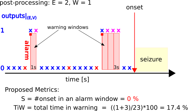
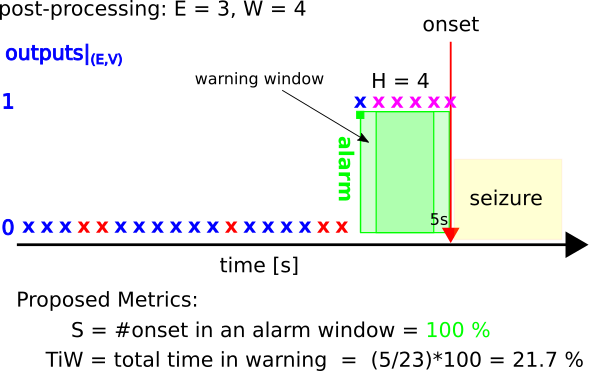
To properly evaluate these performances we kept in mind that an hypothetical portable alarm system or device should raise an alarm on the basis of the classifier output, and this alarm could last in time [40]. Moreover the mapping between the output of the classifier and the resulting alarm could be not only but in general , meaning that at least consecutive positive outputs or events must be achieved by the classifier to let the device raise an alarm.
For this reason, as suggested in [10], we adopted the following metrics: the sensitivity (S), the true positive seizure prediction rate, i.e. if a seizure occurs while the system is in the alarm state then S is equal to ; the time in warning (TiW), the total duration of raised alarms (such red light indicators) in a monitored time window, i.e. if the system never raise an alarm its TiW is and of course the corresponding S is too, on the other side if the system raise alarms in a way that their total duration makes a TiW equal to , surely it will achieve an S of too. Both these cases (system always off or always on) are obviously useless in a real world scenario, but if we consider these extremes as points in the plane with TiW on the x-axis and S on the y-axis, it remains a desirable working zone in the middle of these extremes, above the bisector line identified by
the points that satisfy the equation , or , where is defined as the improvement over chance [10].
In this framework, TiW and S strongly depend on the choice of the two aforementioned parameters: the first is the number of consecutive events labeled as pre-ictal by the classifier, that should be considered by the system or the device to raise an alarm, the second is the alarm duration. In the following we will refer to these parameters as E and W, respectively.
For each classifier we performed a grid search varying E values beween one and ten (events) and W from one second to five minutes with a one-second step, for a total of rounds per classifier computing S, TiW, IoC and prediction horizon (H) when as the time interval between the alarm and the onset.
These metrics have been collected in tensors with dimensions , with the type of classifier, identified by P and O parameters; the number of datasets, the number of permutations on the dataset ( is the number of training sets),
and are E and W respectively. Each metric tensor contains values.

In Figure 10 we report aggregated validation and prediction performances (the former are obtained on each possible permutations of the feature dataset, the latter only on the permutation that preserve the line of time) for each classifier, evaluating the mean sensitivity and the TiW box plots for all datasets and parameters combination in the five classifier groups identified by the P parameter, i.e. the size in seconds of the pre-ictal class.
In Table 1 we report the best validation performances with corresponding mean values obtained from each group of classifiers, for all datasets, permutations and combinations of E and W parameters:
| P | S (%) | TiW (%) | IoC (%) | H (s) | O (s) |
|---|---|---|---|---|---|
| P | S (%) | TiW (%) | IoC (%) | H (s) | O (s) |
|---|---|---|---|---|---|
summarizing the previous results and considering the corresponding mean IoC values, the best performance on all datasets from the validation point of view is achieved by the classifier with the s window starting seconds before the onset, which obtain an IoC equal to , followed by classifier with the second window starting seconds before the onset and IoC equal to , classifier with the s window starting seconds before the onset and an Ioc of , classifier with s window starting s before the onset and IoC equal to and finally classifier with s window starting s before the onset with an IoC of .
| P | S (%) | TiW (%) | IoC (%) | H (s) | O (s) |
|---|---|---|---|---|---|
| P | S (%) | TiW (%) | IoC (%) | H (s) | O (s) |
|---|---|---|---|---|---|
In Table 2 we report the best prediction performances with corresponding mean values obtained from each group of classifiers for all datasets, the permutation that preserve the last seizure as validation and combinations of E and W parameters:
considering IoC values, the best result is still achieved from classifier with the same s offset and an of , little lower than previous, followed by classifier (instead of the previous classifier) with a s offset and IoC equal to , a lower value compared to previous ’s IoC value but higher value than the corresponding previous value; then follow the classifier with a s offset and a IoC, lower than previous value, the classifier with s offset and a Ioc value of , lower than previous but higher than previous and at last with a s offset and Ioc equal to , higher than previous IoC.
Therefore the classifier trained with the last s of pre-ictal samples before the onset reaches the best performance (on average, for all datasets and combinations of E and W parameters) in terms of sensitivity (-) and time in warning (-), in both validation and prediction performances.
We could benchmark this result with the results obtained in [10], corresponding to a mean sensitivity value of the prediction system equal to over a mean time in warning of noting that we achieve a comparable mean sensitivity, dropping at the same time about on the mean time in warning performance. This drop is not surprising considering the different nature of the datasets:
our chosen features are builded upon clinical non-invasive s-EEG data, while data used in the benchmark study are invasive intracranial EEG data, with a huge difference in both data quality and reliability.
| P | S (%) | TiW (%) | IoC (%) | H (s) | O (s) |
|---|---|---|---|---|---|
| P | S (%) | TiW (%) | IoC (%) | H (s) | O (s) |
|---|---|---|---|---|---|
Moreover we could notice that we are not delimiting ranges for E and W parameters, the number of events needed by the system to raise the alarm and the duration of the alarm itself, respectively. If we continue to consider all dataset but restrict E in the set
and W in the set
we obtain the following validation and prediction performances: from Table 3 we find that the best classifier now is, on average, the classifier with offset with respect to the seizure onset, that scores a mean Ioc of over a mean sensitivity of , a mean time in warning of and with a mean prediction horizon of seconds. Comparison with results from Table 1 shows that improvement from the best previous Ioc is mainly due to a substantial descreasing in TiW (from to ) and at the same time a decreasing in S value (from to ).
From the prediction point of view, Table 4 report that best classifier now is with a s offset, reaching an average IoC value of on mean sensitivity equal to and mean time in warning equal to , with a mean prediction horizon of seconds. This mean Ioc value for a classifier is also closer to the mean IoC value scored in [10].
Narrowing further set E in the range lead to the following validation and prediction performances, summarized in Tables 5 and 6, respectively.
The prediction results indicate that the global performance of classifier with s offset could be refined, achieving a mean IoC value of resulting from a mean sensitivity of and a mean TiW of and a mean prediction horizon of about seconds, improving the IoC benchmark obtained in [10] of about , resulting from an increase of in the mean sensitivity and at the same time a decrease of more than in the mean TiW.
Finally, the presented approach allow the possibility to evalute these performances for each dataset separately, addressing in a pseudo-prospective manner the specifity between dataset and dataset. In the following we report in Table 7 validation performance on dataset , considering the previous sets for E and W: on all permutations the best classifier is with s offset, which achieved a mean Ioc value of over a mean sensitivity of and time in warning of , with a mean prediction horizon of seconds.
Considering only the permutation that preserve the line of time, in Table 8 we see for dataset that the best classifier remains but with a closer offset, with an outstanding mean Ioc of over a sensitivity and a mean time in warning and with a prediction horizon of s.
This mean also that, remarkably, a lot of valuable information about the incoming, subject-specific seizure is conveyed in the time interval going from s to s before the seizure onset, and this is exploited by the proposed features.
| P | S (%) | TiW (%) | IoC (%) | H (s) | O (s) |
|---|---|---|---|---|---|
| P | S (%) | TiW (%) | IoC (%) | H (s) | O (s) |
|---|---|---|---|---|---|
| D | S (%) | TiW (%) | IoC (%) | H (s) | P | O (s) |
|---|---|---|---|---|---|---|
This interesting result is reported in Table 9 for each dataset, showing that for these data it does not exists a unique, global classifier configuration, but instead several specific time intervals exist, not necessarily long ones and not necessarily too close to the onset, lasting just or seconds with valuable, predictive power, enabled by the rich pool of the proposed features, over the incoming next seizure.
4 Conclusions
In this work an hybrid approach based on a nonlinear dynamic model on network, namely the EGN, and a nonlinear time series method has been presented with application to the epileptic seizure detection and prediction from real scalp electroencephalogram data.
The proposed mixed approach permits to build, starting from noisy real-world data such as scalp EEG data, a classifier which obtain comparable performances with very recent studies in the field, notably based on invasive intracranial EEG data, in terms of mean sensitivity metric and better performances of the mean time in warning metric, scoring a mean improvement over chance of , against a benchmark value.
Furthermore, results obtained from subject-specific classification revealed novel insights about valuable information in specific short-lasting time intervals before seizure onset, information conveyed by the chosen features, thus reinforcing scalp based approaches, bearing in mind that s-EEG data represent the most obvious source for the development of new wearable warning devices.
However a major difficulty remains concerning the availability of statistically meaningful scalp EEG datasets in comparison with intracranial datasets, in terms of size (number of seizures), quality and reliability of data.
Addressing this point we are currently developing and building a prototype of a portable wearable device for seizure warning and continuous s-EEG recording, on which the proposed methods will be implemented to enhance the pool of available s-EEG seizures and the same toughen the features used.
Acknowledgments
DM, CM and RZ were partially supported by grant PANACEE (Prevision and analysis of brain activity in transitions: epilepsy and sleep) of Regione Toscana (Italy) - PAR FAS 2007-2013 1.1.a.1.1.2 - B22I14000770002.
Conflicts of interest
The authors declare no conflict of interest.
Appendix A - Examples on metrics evaluation

References
- [1] Strogatz, S. H. Nonlinear dynamics and chaos. Westview Press, 1994.
- [2] Madeo, D. Modeling and Identification of Networked and Distributed Complex Systems. Ph.D. Thesis, University of Siena, 2015.
- [3] Hocepied, G., Legros, B., Van Bogaert, P., Grenez, F., Nonclercq, A. Early detection of epileptic seizures based on parameter identification of neural mass model. Comput. Biol. Med. 2013, vol. 43, pp. 1773–1782.
- [4] Kramera, M. A., Kolaczykb, E. D., Kirschc, H. E. Emergent network topology at seizure onset in humans. Epilepsy Research, 2008, vol. 79, iss. 2–3, pp. 173–186.
- [5] Mormann, F., Kreuz, T., Rieke, C., Andrzejak, R. G., Kraskov, A., David, P., … & Lehnertz, K. On the predictability of epileptic seizures. Clinical neurophysiology, 2005, 116(3), 569-587.
- [6] Lehnertz, K., Elger, C. E. Can Epileptic Seizures be Predicted? Evidence from Nonlinear Time Series Analysis of Brain Electrical Activity. Phys. Rev. Lett. 1998, vol. 80, pp. 5019–5022.
- [7] Mormann, F., Andrzejak, R. G., Elger, C. E., & Lehnertz, K. Seizure prediction: the long and winding road. Brain, 2006, 130(2), 314-333.
- [8] Stacey, W.C. Seizure Prediction Is Possible–Now Let’s Make It Practical. EBioMedicine, 2018.
- [9] Karoly, P. J., Ung, H., Grayden, D. B., Kuhlmann, L., Leyde, K., Cook, M. J., & Freestone, D. R. The circadian profile of epilepsy improves seizure forecasting. Brain, 2017, 140(8), 2169-2182.
- [10] Kiral-Kornek, I., Roy, S., Nurse, E., Mashford, B., Karoly, P., Carroll, T., …& Grayden, D. Epileptic seizure prediction using big data and deep learning: toward a mobile system. EBioMedicine, 2017.
- [11] Cook, M. J., O’Brien, T. J., Berkovic, S. F., Murphy, M., Morokoff, A., Fabinyi, G., …& Hosking, S. Prediction of seizure likelihood with a long-term, implanted seizure advisory system in patients with drug-resistant epilepsy: a first-in-man study. The Lancet Neurology, 2013, 12(6), 563-571.
- [12] Nguyen, N. A. T., Yang, H. J., & Kim, S. HOKF: High Order Kalman Filter for Epilepsy Forecasting Modeling. Biosystems, 2017, 158, 57-67.
- [13] Wendling, F., Benquet, P., Bartolomei, F., & Jirsa, V. Computational models of epileptiform activity. Journal of neuroscience methods, 2016, 260, 233-251.
- [14] Aarabi, A., He, B. Seizure prediction in hippocampal and neocortical epilepsy using a model-based approach. Clinical Neurophysiology, 2014, 125(5), 930-940.
- [15] Da Silva, F. L., Blanes, W., Kalitzin, S. N., Parra, J., Suffczynski, P., & Velis, D. N. Epilepsies as dynamical diseases of brain systems: basic models of the transition between normal and epileptic activity. Epilepsia, 2003, 44(s12), 72-83.
- [16] da Silva, F. H. L., Blanes, W., Kalitzin, S. N., Parra, J., Suffczynski, P., & Velis, D. N. Dynamical diseases of brain systems: different routes to epileptic seizures. IEEE Transactions on Biomedical Engineering, 2003, 50(5), 540-548.
- [17] Van Mierlo, P., Papadopoulou, M., Carrette, M. E., Boon, P., Vandenberghe,S., Vonck, K., Marinazzo, D. Functional brain connectivity from EEG in epilepsy: Seizure prediction and epileptogenic focus localization. Progress in Neurobiology, 2014, vol. 121, pp. 19-35.
- [18] Newman, M. E. J. Networks, an Introduction. Oxford University Press, 2010.
- [19] Hofbauer, J., Sigmund, K. Evolutionary games and population dynamics. Cambridge University Press, 1998.
- [20] Madeo, D., Mocenni, C. Game Interactions and dynamics on networked populations. IEEE Trans. on Autom. Control, 2015, vol. 60, is. 7, pp. 1801-1810.
- [21] Iacobelli, G., Madeo, D., & Mocenni, C. Lumping evolutionary game dynamics on networks. Journal of Theoretical Biology. 2016, 407, pp. 328-338.
- [22] Madeo, D., Talarico, A., Pascual-Leone, A., Mocenni, C., & Santarnecchi, E. An Evolutionary Game Theory Model of Spontaneous Brain Functioning. Scientific Reports. 2017, 7(1), 15978.
- [23] Marwan, N., Romano, M. C., Thiel, M., & Kurths, J. Recurrence plots for the analysis of complex systems. Physics reports, 2007, 438(5-6), 237-329.
- [24] Schinkel, S., Marwan, N., & Kurths, J. Brain signal analysis based on recurrences. Journal of Physiology-Paris, 2009, 103(6), 315-323.
- [25] Madeo, D., Castellani, E., Santarcangelo, E. L., Mocenni, C. Hypnotic assessment based on the Recurrence Quantification Analysis of EEG recorded in the ordinary state of conscoiusness. Brain and Cognition, 2013, vol. 83, is. 2, pp. 227-233.
- [26] Becker, K., Schneider, G., Eder, M., Ranft, A., Kochs, E. F., Zieglgänsberger, W., & Dodt, H. U. Anaesthesia monitoring by recurrence quantification analysis of EEG data. PloS one. 2010, 5(1), e8876.
- [27] Thomasson, N., Hoeppner, T. J., Webber Jr, C. L., & Zbilut, J. P. Recurrence quantification in epileptic EEGs. Physics Letters A, 2001, 279(1-2), 94-101.
- [28] Chiarucci, R., Madeo, D., Loffredo, M. I., Castellani, E., Santarcangelo, E. L., & Mocenni, C. Cross-evidence for hypnotic susceptibility through nonlinear measures on EEGs of non-hypnotized subjects. Scientific reports, 2014. 4, 5610.
- [29] Baghdadi, G., Nasrabadi, A. M. Effect of Hypnosis and Hypnotisability on Temporal Correlations of EEG Signals in Different Frequency Bands. European Journal of Clinical Hypnosis, 2009, 9(1).
- [30] Franaszczuk, P. J., Blinowska, K. J. Linear Model of Brain Electrical Activity - EEG as a Superposition of Damped Oscillatory Modes. Biol. Cybern. 1985, vol. 53, pp. 19-25.
- [31] Opsahl, T., Panzarasa, P. Clustering in weighted networks. Social networks, 2009, 31(2), 155-163.
- [32] Zbilut, J. P., & Webber Jr, C. L. Embeddings and delays as derived from quantification of recurrence plots. Physics letters A, 1992, 171(3-4), 199-203.
- [33] Webber Jr, C. L., & Zbilut, J. P. Dynamical assessment of physiological systems and states using recurrence plot strategies. Journal of applied physiology, 1994, 76(2), 965-973.
- [34] Takens, F. Detecting strange attractors in turbulence, in “Dynamical systems and turbulence”. Lect. Notes Math. 1981, 898 366 - 381.
- [35] Trulla, L. L., Giuliani, A., Zbilut, J. P., & Webber Jr, C. L. Recurrence quantification analysis of the logistic equation with transients. Physics Letters A, 1996, 223(4), 255-260.
- [36] Marwan, N., Wessel, N., Meyerfeldt, U., Schirdewan, A., & Kurths, J. Recurrence-plot-based measures of complexity and their application to heart-rate-variability data. Physical review E, 2002, 66(2), 026702.
- [37] Mocenni, C., Facchini, A., & Vicino, A. Identifying the dynamics of complex spatio-temporal systems by spatial recurrence properties. Proceedings of the National Academy of Sciences, 2010, 107(18), 8097-8102.
- [38] Kantz, H., Schreiber, T. Nonlinear time series analysis (Vol. 7). Cambridge university press. 2004.
- [39] Bradley, E., Kantz, H. Nonlinear time-series analysis revisited. Chaos: An Interdisciplinary Journal of Nonlinear Science, 2015, 25(9), 097610.
- [40] Snyder, D. E., Echauz, J., Grimes, D. B., & Litt, B. The statistics of a practical seizure warning system. Journal of neural engineering, 2008, 5(4), 392.
- [41] Russell, S. J., Norvig, P., Canny, J. F., Malik, J. M., & Edwards, D. D. Artificial intelligence: a modern approach 2003, (Vol. 2, No. 9). Upper Saddle River: Prentice hall.
- [42] Hastie, T., Tibshirani, R. & Friedman, J. The Elements of Statistical Learning. 2001. New York: Springer.