Bayesian Analysis of Nonparanormal Graphical Models Using Rank-LikelihoodJournal: Journal of LaTeX Templates

Graphical models are useful mathematical tools that model complex dependence relationships between variables. Under the Gaussianity assumption, the graph of relations is completely determined by the zeros in the inverse covariance matrix, also known as the precision matrix. If the $(i,j)$th entry of the precision matrix is zero, then the $i$th and the $j$th variables are conditionally independent given all other variables; see Lauritzen 1996 and Edwards 2000 for more information on the properties of Gaussian graphical models (GGMs).

If the variables are not normally distributed, an adjustment needs to be made if one wants to use the statistical properties of a Gaussian graphical model. The standard procedure is to transform the data, typically by the logarithmic or the square root transformation. With such transformations, one has to check each transformation to see if the data appear close to normal, checking which can be tedious and the method is somewhat ad-hoc. From a modeling perspective, an easier solution is to leave the transformation functions unspecified and estimate them instead. The nonparanormal graphical model [Liu et al. 2009] consists of estimating the transformation functions using a truncated marginal empirical distribution function, and then estimating the precision matrix of the transformed variables using the graphical lasso assuming sparsity. A Bayesian approach for nonparanormal graphical models, developed by Mulgrave and Ghosal 2018a, Mulgrave and Ghosal 2018b, uses a random series B-splines prior to estimate the transformation functions and induces sparsity on the off-diagonal entries of the precision matrix by spike-and-slab or continuous shrinkage priors, either directly or through the Cholesky decomposition.

However, one important requirement of the nonparanormal model is that the transformation functions need to be estimated. In order to avoid estimating the transformation functions, alternative rank-based procedures can be employed to transform the data to normally distributed random variables. Dabrowska and Doksum 1988 study the properties of the likelihood function based on transformed observations in a general class called transformation models. An example is given by the rank-likelihood which is the joint distribution of the ranks of the observations. The rank-likelihood is invariant under monotone transformations of the observations. Thus one can ignore the transformations and focus on the main parameter of interest, the precision matrix, or equivalently, the inverse correlation matrix. The rank-likelihood has been used for semiparametric copula estimation [Hoff 2007], for Receiver Operating Characteristic (ROC) curve estimation [Gu and Ghosal 2009, Gu et al. 2014], and for ROC surface estimation [Zhu and Ghosal 2019]. The use of the rank-likelihood results in a gain in robustness and simplification of estimation. Models which can be represented by transformations on Gaussian graphical models are generally known as Gaussian copula graphical models (GCGMs) and have been explored in the Bayesian literature [Pitt et al. 2006, Dobra and Lenkoski 2011, Liu et al. 2012, Mohammadi and Wit 2017]. In the frequentist literature, nonparametric rank-based correlation coefficient estimators have been used to construct GCGMs [Liu et al. 2012, Xue and Zou 2012]. These models can also address binary or ordinal data, but we do not pursue this direction here.

Once the transformed variables have been obtained, one needs to estimate a sparse precision matrix in order to learn the structure of the graphical model. In the frequentist literature, the popular algorithm to use is the graphical lasso [Friedman et al. 2008]. Numerous algorithms have been proposed to solve this problem [Meinshausen and Buhlmann 2006, Yuan and Lin 2007, Friedman et al. 2008, Rothman et al. 2008, Banerjee et al. 2008, d’Aspremont et al. 2008, Lu 2009, Scheinberg et al. 2010, Witten et al. 2011, Mazumder and Hastie 2012b]. Alternative penalties used to estimate the sparse precision matrix include adaptive LASSO and SCAD penalties [Fan et al. 2009], and LASSO and grouped LASSO penalties [Friedman et al. 2010]. In the Bayesian literature, graphical models can be learned with the use of continuous shrinkage priors. Priors such as the double exponential [Wang 2012, Peterson et al. 2013], uniform shrinkage priors [Wang and Pillai 2013], and spike-and-slab priors [Wang 2015, Peterson et al. 2016, Li and McCormick 2017, Li et al. 2017, Mulgrave and Ghosal 2018a] can characterize zero and non-zero elements of the precision matrix with continuous distributions that have a mass at zero and heavy tails. More recently, horseshoe priors have been employed for sparse precision estimation [Mulgrave and Ghosal 2018b, Williams et al. 2018]. We estimate a sparse precision matrix using a Cholesky decomposition to naturally incorporate the positive definite matrix, a horseshoe prior to regularize the matrix, and a loss procedure to threshold the matrix. Our methods differ from other Bayesian GCGMs which use the rank-likelihood to transform the random variables. Dobra and Lenkoski 2011 use a G-Wishart prior [Roverato 2002] and Markov Chain Monte Carlo (MCMC) to estimate the sparse precision matrix to construct a GCGM. Mohammadi et al. 2017 estimate a sparse precision matrix using a G-Wishart prior and birth-and-death MCMC [Mohammadi and Wit 2015]. Li and McCormick 2017 put a normal spike-and-slab prior on the precision matrix and use an expectation-conditional maximization algorithm for estimation.

The paper is organized as follows. In the next section, we state model and prior. In Section 3, we review the posterior computation. In Section 4, we review the thresholding procedure and in Section 5, we discuss our tuning procedure. We derive a posterior consistency result in Section 6 and in Section 7, we review the results of the simulation study. Lastly, in Section 8, we describe an application with gene expression data.

We obtain samples of $\textup{Pr}(\bm{\Psi}|\bm{Y}\in D)$ by employing the following Gibbs sampler:

1. 1.

   Sample $\bm{Y}\sim\mathrm{N}(\mathbf{0},\bm{\Psi}^{-1}):$

   For $d=1,\ldots,p$,

   1. (a)

      Compute the ranks of $\bm{X}_{d}$, where $r=1,\ldots,n$ represents the ranks.

      For $r=1,\ldots,n,$

      1. (i)

         Compute $y_{\textup{lower}}=y_{i_{r-1},d}$ and $y_{\textup{upper}}=y_{i_{r+1},d}$, where $i$ is the index for the position of the $r$-th rank of $\bm{X}_{d}$. Let $y_{i_{0},d}=-\infty$ and $y_{i_{n+1},d}=\infty$.

      2. (ii)

         Compute $\mu_{i_{r},d}=-\bm{\psi}_{d,d}^{-1}\bm{\Psi}_{d,\setminus d}\bm{Y}_{i_{r},\setminus d}$

      3. (iii)

         $\sigma_{d}^{2}=\bm{\psi}_{d,d}^{-1}$

      4. (iv)

         Sample $Y_{i_{r},d}\sim\mathrm{TN}(\mu_{i_{r},d},\sigma_{d}^{2};\;y_{\textup{lower}}<Y_{i_{r},d}<y_{\textup{upper}}),$ where
         $\mathrm{TN}(a,b;\;c<x<d)$ denotes a univariate truncated normal distribution with mean $a$, variance $b$, and truncation limits $c$ and $d$. Sampling from the truncated normal distribution is implemented with the fast sampling function trandn in MATLAB that uses minimax tilting [Botev 2017].

2. 2.

   Sample $\bm{\Omega}$:

   For $d=1,\ldots,p-1,$

   1. (a)

      Sample the variables $\bm{\beta}_{k>d}|(\sigma_{d},\bm{b}_{k>d},\lambda_{d}^{2})\sim\mathrm{N}(\bm{A}^{-1}\bm{Y}_{k>d}^{T}\bm{Y}_{d},\sigma_{d}^{2}\bm{A}^{-1})$, where
      $\bm{A}=(\bm{Y}_{k>d}^{\prime}\bm{Y}_{k>d}+\textup{diag}({p^{2}k}/({\lambda_{d}^{2}\bm{b}_{k>d}c^{2}}))).$

      Since sampling from this normal distribution can be expensive with large $p$, we used an exact sampling algorithm for Gaussian priors that uses data augmentation [Bhattacharya et al. 2016]:

      1. (i)

         Sample $t\sim\mathrm{N}(\mathbf{0},\bm{D})$ and $\delta\sim\mathrm{N}(0,I_{n})$, where $\bm{D}=\displaystyle\sigma_{d}^{2}\textup{diag}(\frac{\lambda_{d}^{2}\bm{b}_{k>d}c^{2}}{p^{2}k});$

      2. (ii)

         set $v=\bm{\Phi}t+\delta$, where $\bm{\Phi}=\bm{Y}_{k>d}/\sigma_{d};$

      3. (iii)

         solve $(\bm{\Phi}\bm{D}\bm{\Phi}^{\prime}+\bm{I}_{n})w=(\alpha-v)$, where $\alpha=\textbf{Y}_{d}/\sigma_{d};$

      4. (iv)

         set $\beta=t+\bm{D}\bm{\Phi}^{\prime}w.$

   2. (b)

      Sample $\lambda_{d}^{2}\sim\mathrm{IG}(\displaystyle\frac{\#(k>d)}{2}+\frac{1}{2},\frac{1}{2}\bm{\beta}_{k>d}^{\prime}\textup{diag}(\frac{p^{2}k}{\sigma_{d}^{2}\bm{b}_{k>d}c^{2}})\bm{\beta}_{k>d}+\frac{1}{a_{d}}).$

   3. (c)

      Sample $a_{d}\sim\mathrm{IG}(1,\lambda_{d}^{-2}+1).$

   4. (d)

      Sample $b_{kd}\sim\mathrm{IG}(1,\frac{p^{2}k\beta_{kd}^{2}}{2\sigma_{d}^{2}\lambda_{d}^{2}c^{2}}+\frac{1}{h_{kd}}).$

   5. (e)

      Sample $h_{kd}\sim\mathrm{IG}(1,\frac{1}{b_{kd}}+1).$

   6. (f)

      Sample $\sigma_{d}^{2}\sim\mathrm{IG}(\frac{n+\#(k>d)}{2}+0.01,\frac{1}{2}\left\|\bm{Y}_{d}-\bm{Y}_{k>d}\bm{\beta}_{k>d}\right\|^{2}$
      $+\frac{1}{2}\bm{\beta}_{k>d}^{\prime}\textup{diag}(\frac{p^{2}k}{\lambda_{d}^{2}\bm{b}_{k>d}c^{2}})\bm{\beta}_{k>d}+0.01).$ Sample $\sigma_{p}^{2}\sim\mathrm{IG}({n}/{2}+0.01,1/2\left\|\bm{Y}_{p}\right\|^{2}+0.01).$

   7. (g)

      Compute $l_{kd}=-\beta_{kd}/\sigma_{d}\textup{ and }l_{dd}=1/\sigma_{d}.$

   8. (h)

      Compute $\bm{\Omega}=\textbf{L}\textbf{L}^{\prime}.$

3. 3.

   Set $\bm{\Psi}=\bm{A}\bm{\Omega}\bm{A}$, where $\bm{A}=\textup{diag}(\sigma_{dd})$ and $\sigma_{dd}$ are the square roots of the diagonal elements of $\bm{\Sigma}=\bm{\Omega}^{-1}$.

These steps are repeated until convergence.

For the sparsity constraint on the inverse correlation matrix $\bm{\Psi}$, we need to select the value of the parameter $c$. We solve a convex constrained optimization problem in order to use the Bayesian Information Criterion (BIC), originally described in Dahl et al. 2005, Dahl et al. 2008 and developed further in Mulgrave and Ghosal 2018a. First, we find the Bayes estimate of the inverse correlation matrix, $\hat{\bm{\Psi}}=\mathrm{E}(\bm{\Psi}|\bm{Y})$. We also find the average of the transformed variables, $\bar{\bm{Y}}=M^{-1}\sum_{m=1}^{M}\bm{Y}_{m}$, where $\bm{Y}_{m}$, $m=1,\ldots,M$, are obtained from the MCMC output. Then, using the sum of squares matrix, $\bm{S}=\bar{\bm{Y}}^{\prime}\bar{\bm{Y}}$, we solve the following to obtain the maximum likelihood estimate of the inverse correlation matrix, $\hat{\bm{\Psi}}_{\mathrm{MLE}}$:

where $\mathcal{C}$ stands for the constraint that an element of $\bm{\Psi}$ is zero if and only if the estimated edge matrix from the MCMC sampler has that element as zero. The estimated edge matrix from the MCMC sampler will be described in more detail in Subsection 7.1. For computational simplicity, in the code, we represent this problem as an unconstrained optimization problem as described in Dahl et al. 2005, Dahl et al. 2008.

Lastly, we calculate $\textup{BIC}=-2\ell(\hat{\bm{\Psi}}_{\mathrm{MLE}})+k\log n$, where $k=\#\mathcal{C}(\hat{\bm{\Psi}}_{\mathrm{MLE}})$, the sum of the number of diagonal elements and the number of edges in the estimated edge matrix, and $-\ell(\hat{\bm{\Psi}}_{\mathrm{MLE}})=-n\log\det\hat{\bm{\Psi}}_{\mathrm{MLE}}+\textup{tr}(\hat{\bm{\Psi}}_{\mathrm{MLE}}\textbf{S})$. We select the $c$ that results in the smallest BIC.

In this section, we show that in the fixed dimensional setting (i.e. $p$ is fixed), the rank-based posterior distribution of $\bm{\Psi}$ is consistent at its true value $\bm{\Psi}_{0}$ for almost all $\bm{\Psi}_{0}$ with respect to the Lebesgue measure under the only assumption that the prior distribution for $\bm{\Psi}$ has positive density on the space of inverse correlation matrices, i.e., the collection of all $p\times p$ positive definite matrices $\bm{\Psi}$ such that all diagonal elements of $\bm{\Psi}^{-1}$ are $1$.

Usually, the main criticism against a posterior consistency result obtained by applying Doob’s theorem is that the exceptional set where consistency may fail may be “large” since it only needs to be null with respect to the prior, which is somewhat arbitrary. However, in the present application, since the parameter space for the parameter of interest $\bm{\Psi}$ is finite dimensional, where we have the Lebesgue measure as a benchmark measure, the exceptional set of points where the posterior may be inconsistent is characterized as Lebesgue null, which can be regarded as “small”. It is important to note that the normality restoring transformations are taken to be fixed, and no prior is assigned on them. Since the underlying procedure is unaffected by the transformations, the fact that these transformations are unknown does not matter. Note that the fixed dimensionality of the variables is essential since the posterior consistency result is applicable only if the parameter space is fixed.

We conduct a simulation study to compare the performance of the proposed Bayesian rank-likelihood method, the Bayesian GCGM [Mohammadi et al. 2017], the empirical method in a nonparanormal graphical model [Liu et al. 2009], the Bayesian method in a nonparanormal graphical model [Mulgrave and Ghosal 2018b], and the empirical method based on GCGM [Liu et al. 2012]. Both the proposed Bayesian rank-likelihood method, indicated as Rank-Likelihood, and the Bayesian method of Mulgrave and Ghosal 2018b, indicated as B-splines, use a horseshoe prior on the Cholesky decomposition of the precision matrix and MCMC estimation. The B-splines method uses a random series B-splines prior to estimate the transformation functions. The Bayesian method based on GCGM, indicated as Bayesian Copula, uses the rank-likelihood to transform the random variables and puts a G-Wishart prior on the inverse correlation matrix, a uniform prior on the graph, and estimates the sparse matrix using a birth-and-death MCMC [Mohammadi and Wit 2015]. The empirical method in a nonparanormal graphical model, indicated as Truncation, uses a truncated marginal empirical distribution function to transform the variables and the graphical lasso to estimate the sparse precision matrix. The empirical method based on GCGM, indicated as SKEPTIC, uses Spearman’s rho to transform the variables and estimates the sparse precision matrix with the graphical lasso.

The random variables, $Y_{1},\ldots,Y_{p}$, are simulated from a multivariate normal distribution such that $Y_{i1},\ldots,Y_{ip}\stackrel{{\scriptstyle\mathrm{i.i.d.}}}{{\sim}}\mathrm{N}(\bm{\mu},\bm{\Omega}^{-1})$ for $i=1,\ldots,n$. The means $\bm{\mu}$ are selected from an equally spaced grid between 0 and 5 with length $p$. We consider nine different combinations of $n,p,$ and sparsity for $\bm{\Omega}$:

• 1.

  $p=25,\;n=50$, AR(4) model;

• 2.

  $p=50$, $n=100$, AR(4) model;

• 3.

  $p=100$, $n=500$, AR(4) model;

• 4.

  $p=25,\;n=50$, AR(1) model;

• 5.

  $p=50$, $n=100$, AR(1) model;

• 6.

  $p=100$, $n=500$, AR(1) model;

• 7.

  $p=25$, $n=50$, sparsity = $10\%$ non-zero entries in the off-diagonals;

• 8.

  $p=50$, $n=100$, sparsity = $5\%$ non-zero entries in the off-diagonals;

• 9.

  $p=100$, $n=500$, sparsity = $2\%$ non-zero entries in the off-diagonals;

where the AR(4), AR(1), and star models are described by the relations

• 1.

  AR(4) model: $\omega_{i,i}=1,\;\omega_{i,i-1}=\omega_{i-1,i}=0.2,\;\omega_{i,i-2}=\omega_{i-2,i}=0.2,\;\omega_{i,i-3}=\omega_{i-3,i}=0.2,\;\omega_{i,i-4}=\omega_{i-4,i}=0.1$;

• 2.

  AR(1) model: $\omega_{1,1}=1.9608,\;\omega_{i,i-1}=\omega_{i-1,i}=-1.3725$, $\omega_{p,p}=1.9608$

The percent sparsity levels for $\bm{\Omega}$ are computed using lower triangular matrices that have diagonal entries normally distributed with mean 1 and standard deviation 0.1, and non-zero off-diagonal entries normally distributed with mean 0 and standard deviation 1.

The observed variables $\bm{X}=(X_{1},\ldots,X_{p})$ are constructed from the simulated variables $Y_{1},\ldots,Y_{p}$. The functions used to construct the observed variables were four cumulative distribution functions (c.d.f.s): asymmetric Laplace, extreme value, logistic, and stable. We could choose any values of the parameters for the c.d.f.s, but instead of selecting them ourselves, we automatically choose the values of the parameters to be the maximum likelihood estimates with the mle function in MATLAB. The values of the parameters for each of the c.d.f.s are the maximum likelihood estimates for the parameters of the corresponding distributions (asymmetric Laplace, extreme value, logistic, and stable), using the variables $Y_{1},\ldots,Y_{p}$.

We follow the procedure in Mulgrave and Ghosal 2018a to estimate the transformation functions for the B-splines method. The hyperparameters for the normal prior are chosen to be $\nu=1,\tau=1,$ and $\sigma^{2}=1$. To choose the number of basis functions, we use the Aikaike Information Criterion. Samples from the truncated multivariate normal posterior distributions for the B-spline coefficients are obtained using the exact Hamiltonian Monte Carlo (exact HMC) algorithm [Pakman and Paninski 2014]. After finding the initial coefficient values $\bm{\theta}_{d}$, we construct initial values for $Y_{d,\textup{initial}}=\sum_{j=1}^{J}\theta_{dj,\textup{initial}}B_{j}(X_{d})$ using the observed variables. These initial values $\bm{Y}_{\textup{initial}}$ are used to find initial values for $\bm{\Sigma},\bm{\mu}$, and $\bm{\Omega}$ for the algorithm.

For the Rank-Likelihood method, we initialize the algorithm using the ranks of the observed variables. First, we create a $p\times n$ matrix of ranks, $\bm{R}=\mbox{rank}(\bm{X})$. Then, we divide the columns by $n+1$ and transform each entry by the standard normal quantile function using the inverse standard normal c.d.f., such that $\bm{Y}_{\textup{initial}}=\bm{\Phi}^{-1}(\bm{R}/(n+1))^{\prime}$. Finally, we take the transpose to obtain an $n\times p$ matrix. We obtain an initial value for the inverse correlation matrix using $\bm{\Psi}_{\textup{initial}}=(\mbox{corr}(\bm{Y}_{\textup{initial}}))^{-1},$ where corr stands for the correlation coefficients of $\bm{Y}_{\textup{initial}}.$

For both the Rank-Likelihood and the B-splines methods, the hyperparameters for the horseshoe prior are initialized with ones. To impose the sparsity constraint on the Cholesky decomposition of the matrices for the B-splines and the Rank-Likelihood methods, we consider four values for tuning: $c\in\{0.1,1,10,100\}$. We select the graphical model with the value of $c$ having the lowest BIC. The 0-1 loss procedure (4.1) is used to threshold the matrices for the B-splines and the Rank-Likelihood methods and construct the corresponding edge matrices. The codes for these methods are written in MATLAB.

For the simulation study, we run 100 replications for each of the nine combinations and assess structure learning and parameter estimation for each replication. We collect $10000$ MCMC samples for inference after discarding a burn-in of $5000$ and we do not apply thinning. The Bayesian Copula method is implemented in the R package BDgraph [Mohammadi and Wit 2017, Mohammadi and Wit 2019] using the option “gcgm”. Bayesian model averaging is used for inverse correlation matrix and graph selection. The default option in the BDgraph package selects the graph formed by links having estimated posterior probabilities greater than $0.5$. The Truncation and SKEPTIC methods are implemented in the R package huge [Zhao et al. 2015] using the “truncation” and “skeptic” options respectively. For both empirical methods, the graphical lasso method is used for the graph estimation based on transformed variables and the default lossless screening method [Witten et al. 2011, Mazumder and Hastie 2012a] is applied. A sequence of 100 regularization parameters, $\lambda$, is generated starting from $\lambda_{\mbox{max}}$ to $0.01*\lambda_{\mbox{max}}$, in the log-scale. We define $\lambda_{\mbox{max}}=\max(\max(\bm{M}-\mbox{diag}(p)),-\min(\bm{M}-\mbox{diag}(p)))$, where $\bm{M}$ is the correlation matrix from the SKEPTIC method and $\bm{M}$ is the matrix constructed for the Truncation method after scaling the transformed variables and converting it to a correlation matrix. Note that $p$ is the dimension. The method used to select the graphical model along the regularization path is Generalized Stability Approach to Regularization Selection [Müller et al. 2016], or G-StARS, implemented using the R package pulsar. We use upper and lower bounds to reduce the computational burden and the number of random subsamples taken for graph re-estimation was 100. All codes are provided in the Supplementary Material.

We demonstrate the methods on a gene expression data set originally referenced in Stranger et al. 2007 with Gene Expression Omnibus database Series Accession Number GSE6536 19 and its funding is supported in part by the US National Institutes of Health ENDGAME. Data are collected to measure the gene expression in B-lymphocyte cells from inhabitants in Utah with European ancestry. The interest is on the single nucleotide polymorphisms that are found in the 5’ untranslated region of messenger RNA with a minor allele frequency $\geq 0.1$. Following Bhadra and Mallick 2013, of the 47,293 total available probes, we considered the 100 most variable probes that correspond to different Illumina TargetID transcripts. The data for these 100 transcripts are available in the R package BDgraph [Mohammadi and Wit 2017, Mohammadi and Wit 2019]. The data consist of $n=60$ unrelated individuals and $p=100$ transcripts. The variables in the data are continuous but do not appear Gaussian. A Bayesian estimate based on a Gaussian graphical model using a spike-and-slab type prior constructed by Bhadra and Mallick 2013 detected 55 edges.

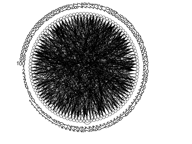
To construct the graph using our method, we convert the original values to be between 0 and 1 using the affine transform $({x-\min(x_{i})})/({\max(x_{i})-\min(x_{i})})$. We use the identity matrix as the initial matrix for the covariance and inverse covariance matrices for the Rank-Likelihood and B-splines methods. The Rank-Likelihood method results in 252 edges and the B-splines method results in 99 edges. Convergence of the Rank-Likelihood method can be obtained in about 28 minutes and for the B-splines method in about 60 minutes for a given $c$ for these data on a laptop computer with an Intel i7 processor and 24 GB of RAM. Using the same set-up as in the simulation study, the SKEPTIC method results in no edges and the Truncation method results in 363 edges. The Bayesian Copula method results in 834 edges. The proposed Rank-Likelihood and B-splines methods result in the sparsest models, with the B-splines method as the most sparse model. The graphs of the proposed methods are shown in Figure 1. The graphs of the Bayesian Copula and truncation methods are shown in Figure 2. Since the SKEPTIC method resulted in no edges, it is not included in the comparison. Plots are made with the circularGraph function in MATLAB.

SUPPLEMENTAL MATERIALS

GitHub Repository:

The code for the methods described in this paper can be found in the following GitHub repository: https://github.com/jnj2102/RankLikelihood.

References

- Baldi et al. [2000] Baldi, P., Brunak, S., Chauvin, Y., Andersen, C.A.F., Nielsen, H., 2000. Assessing the accuracy of prediction algorithms for classification: an overview. Bioinformatics 16, 412–424. URL: http://bioinformatics.oxfordjournals.org/cgi/doi/10.1093/bioinformatics/16.5.412, doi:10.1093/bioinformatics/16.5.412.
- Banerjee et al. [2008] Banerjee, O., El Ghaoui, L., d’Aspremont, A., 2008. Model selection through sparse maximum likelihood estimation for multivariate Gaussian or binary data. Journal of Machine Learning Research 9, 485–516. URL: http://dl.acm.org/citation.cfm?id=1390681.1390696.
- Berger and Barbieri [2004] Berger, J.O., Barbieri, M.M., 2004. Optimal predictive model selection. The Annals of Statistics 32, 870–897. URL: http://projecteuclid.org/euclid.aos/1085408489, doi:10.1214/009053604000000238.
- Bhadra and Mallick [2013] Bhadra, A., Mallick, B.K., 2013. Joint high-dimensional Bayesian variable and covariance selection with an application to eQTL analysis. Biometrics 69, 447–457. URL: http://doi.wiley.com/10.1111/biom.12021, doi:10.1111/biom.12021.
- Bhattacharya et al. [2016] Bhattacharya, A., Chakraborty, A., Mallick, B.K., 2016. Fast sampling with Gaussian scale-mixture priors in high-dimensional regression. Biometrika 103, 985–991. doi:10.1093/biomet/asw042.
- Botev [2017] Botev, Z.I., 2017. The normal law under linear restrictions: simulation and estimation via minimax tilting. Journal of the Royal Statistical Society: Series B (Statistical Methodology) 79, 125–148. URL: http://doi.wiley.com/10.1111/rssb.12162, doi:10.1111/rssb.12162.
- Dabrowska and Doksum [1988] Dabrowska, D.M., Doksum, K.A., 1988. Partial likelihood in transformation models with censored data. Scandinavian Journal of Statistics 15, 1–23. URL: http://www.jstor.org/stable/4616080.
- Dahl et al. [2005] Dahl, J., Roychowdhury, V., Vandenberghe, L., 2005. Maximum likelihood estimation of Gaussian graphical models: numerical implementation and topology selection. Technical report, University of California, Los Angeles. URL: http://www.seas.ucla.edu/˜vandenbe/publications/covsel1.pdf.
- Dahl et al. [2008] Dahl, J., Vandenberghe, L., Roychowdhury, V., 2008. Covariance selection for nonchordal graphs via chordal embedding. Optimization Methods and Software 23, 501–520. URL: http://www.tandfonline.com/doi/abs/10.1080/10556780802102693, doi:10.1080/10556780802102693.
- d’Aspremont et al. [2008] d’Aspremont, A., Banerjee, O., El Ghaoui, L., 2008. First-order methods for sparse covariance selection. SIAM Journal on Matrix Analysis and Applications 30, 56–66. URL: http://epubs.siam.org/doi/abs/10.1137/060670985, doi:10.1137/060670985.
- Dobra and Lenkoski [2011] Dobra, A., Lenkoski, A., 2011. Copula Gaussian graphical models and their application to modeling functional disability data. The Annals of Applied Statistics 5, 969–993. URL: http://projecteuclid.org/euclid.aoas/1310562213, doi:10.1214/10-AOAS397.
- Edwards [2000] Edwards, D., 2000. Introduction to Graphical Modelling. Springer Texts in Statistics, Springer New York. URL: https://books.google.com/books?id=gzKumy4BXoQC.
- Fan et al. [2009] Fan, J., Feng, Y., Wu, Y., 2009. Network exploration via the adaptive LASSO and SCAD penalties. The Annals of Applied Statistics 3, 521–541. URL: http://projecteuclid.org/euclid.aoas/1245676184, doi:10.1214/08-AOAS215.
- Friedman et al. [2008] Friedman, J., Hastie, T., Tibshirani, R., 2008. Sparse inverse covariance estimation with the graphical lasso. Biostatistics 9, 432–441. URL: http://biostatistics.oxfordjournals.org/cgi/doi/10.1093/biostatistics/kxm045, doi:10.1093/biostatistics/kxm045.
- Friedman et al. [2010] Friedman, J.S., Hastie, T.J., Tibshirani, R., 2010. Applications of the lasso and grouped lasso to the estimation of sparse graphical models. Technical report, Stanford. URL: http://statweb.stanford.edu/˜tibs/ftp/ggraph.pdf.
- Ghosal and van der Vaart [2017] Ghosal, S., van der Vaart, A., 2017. Fundamentals of Nonparametric Bayesian Inference. Cambridge Series in Statistical and Probabilistic Mathematics (44), Cambridge University Press, Cambridge. URL: http://ebooks.cambridge.org/ref/id/CBO9781139029834.
- Gu and Ghosal [2009] Gu, J., Ghosal, S., 2009. Bayesian ROC curve estimation under binormality using a rank likelihood. Journal of Statistical Planning and Inference 139, 2076–2083. URL: http://linkinghub.elsevier.com/retrieve/pii/S0378375808003819, doi:10.1016/j.jspi.2008.09.014.
- Gu et al. [2014] Gu, J., Ghosal, S., Kleiner, D.E., 2014. Bayesian ROC curve estimation under verification bias. Statistics in Medicine 33, 5081–5096. URL: http://doi.wiley.com/10.1002/sim.6297, doi:10.1002/sim.6297.
- Hoff [2007] Hoff, D., P., 2007. Extending the rank likelihood for semiparametric copula estimation. The Annals of Applied Statistics 1, 265–283. URL: http://projecteuclid.org/euclid.aoas/1183143739, doi:10.1214/07-AOAS107.
- Hájek and Šidák [1967] Hájek, J., Šidák, Z., 1967. Theory of Rank Tests. Academic Press, New York.
- Lauritzen [1996] Lauritzen, S.L., 1996. Graphical models. Number 17 in Oxford statistical science series, Clarendon Press ; Oxford University Press, Oxford : New York.
- Li and McCormick [2017] Li, Z., McCormick, T.H., 2017. An expectation conditional maximization approach for Gaussian graphical models. arXiv preprint arXiv:1709.06970. URL: https://arxiv.org/abs/1709.06970.
- Li et al. [2017] Li, Z.R., McCormick, T.H., Clark, S.J., 2017. Bayesian latent Gaussian graphical models for mixed data with marginal prior information. arXiv preprint arXiv:1711.00877. URL: https://arxiv.org/abs/1711.00877.
- Liu et al. [2012] Liu, H., Han, F., Yuan, M., Lafferty, J., Wasserman, L., 2012. High-dimensional semiparametric Gaussian copula graphical models. The Annals of Statistics 40, 2293–2326. URL: http://www.jstor.org/stable/41806536.
- Liu et al. [2009] Liu, H., Lafferty, J.D., Wasserman, L.A., 2009. The nonparanormal: semiparametric estimation of high dimensional undirected graphs. Journal of Machine Learning Research 10, 2295–2328. URL: http://jmlr.csail.mit.edu/papers/volume10/liu09a/liu09a.pdf.
- Lu [2009] Lu, Z., 2009. Smooth optimization approach for sparse covariance selection. SIAM Journal on Optimization 19, 1807–1827. URL: http://epubs.siam.org/doi/10.1137/070695915, doi:10.1137/070695915.
- Mazumder and Hastie [2012a] Mazumder, R., Hastie, T., 2012a. Exact covariance thresholding into connected components for large-scale graphical lasso. Journal of Machine Learning Research 13, 781–794.
- Mazumder and Hastie [2012b] Mazumder, R., Hastie, T., 2012b. The graphical lasso: new insights and alternatives. Electronic Journal of Statistics 6, 2125–2149. URL: http://projecteuclid.org/euclid.ejs/1352470831, doi:10.1214/12-EJS740.
- Meinshausen and Buhlmann [2006] Meinshausen, N., Buhlmann, P., 2006. High-dimensional graphs and variable selection with the lasso. The Annals of Statistics 34, 1436–1462. URL: http://projecteuclid.org/Dienst/getRecord?id=euclid.aos/1152540754/, doi:10.1214/009053606000000281.
- Mohammadi et al. [2017] Mohammadi, A., Abegaz, F., van den Heuvel, E., Wit, E.C., 2017. Bayesian modelling of Dupuytren disease by using Gaussian copula graphical models. Journal of the Royal Statistical Society: Series C (Applied Statistics) 66, 629–645. URL: http://doi.wiley.com/10.1111/rssc.12171, doi:10.1111/rssc.12171.
- Mohammadi and Wit [2015] Mohammadi, A., Wit, E.C., 2015. Bayesian structure learning in sparse Gaussian graphical models. Bayesian Analysis 10, 109–138. doi:10.1214/14-BA889.
- Mohammadi and Wit [2017] Mohammadi, R., Wit, E.C., 2017. BDgraph: an R package for Bayesian structure learning in graphical models. arXiv preprint arXiv:1501.05108. URL: https://arxiv.org/abs/1501.05108.
- Mohammadi and Wit [2019] Mohammadi, R., Wit, E.C., 2019. BDgraph: Bayesian structure learning in graphical models using birth-death MCMC. R package version 2.57.
- Mulgrave and Ghosal [2018a] Mulgrave, J.J., Ghosal, S., 2018a. Bayesian inference in nonparanormal graphical models. arXiv preprint arXiv:1806.04334. URL: https://arxiv.org/abs/1806.04334.
- Mulgrave and Ghosal [2018b] Mulgrave, J.J., Ghosal, S., 2018b. Regression based Bayesian approach for nonparanormal graphical models. arXiv preprint arXiv:1812.04442. URL: https://arxiv.org/abs/1812.04442.
- Müller et al. [2016] Müller, C.L., Bonneau, R.A., Kurtz, Z.D., 2016. Generalized stability approach for regularized graphical models. arXiv preprint arXiv: 1605.07072. URL: https://arxiv.org/abs/1605.07072.
- Neville et al. [2014] Neville, S.E., Ormerod, J.T., Wand, M.P., 2014. Mean field variational Bayes for continuous sparse signal shrinkage: Pitfalls and remedies. Electronic Journal of Statistics 8, 1113–1151. URL: http://projecteuclid.org/euclid.ejs/1407415580, doi:10.1214/14-EJS910.
- Pakman and Paninski [2014] Pakman, A., Paninski, L., 2014. Exact Hamiltonian Monte Carlo for truncated multivariate Gaussians. Journal of Computational and Graphical Statistics 23, 518–542. URL: http://www.tandfonline.com/doi/abs/10.1080/10618600.2013.788448, doi:10.1080/10618600.2013.788448.
- van der Pas et al. [2014] van der Pas, S.L., Kleijn, B.J.K., van der Vaart, A.W., 2014. The horseshoe estimator: posterior concentration around nearly black vectors. Electronic Journal of Statistics 8, 2585–2618. URL: https://projecteuclid.org:443/euclid.ejs/1418134265, doi:10.1214/14-EJS962.
- Peterson et al. [2013] Peterson, C., Vannucci, M., Karakas, C., Choi, W., Ma, L., Maletic-Savatic, M., 2013. Inferring metabolic networks using the Bayesian adaptive graphical lasso with informative priors. Statistics and Its Interface 6, 547–558. URL: http://www.intlpress.com/site/pub/pages/journals/items/sii/content/vols/0006/0004/a012/, doi:10.4310/SII.2013.v6.n4.a12.
- Peterson et al. [2016] Peterson, C.B., Stingo, F.C., Vannucci, M., 2016. Joint Bayesian variable and graph selection for regression models with network-structured predictors. Statistics in Medicine 35, 1017–1031. URL: http://doi.wiley.com/10.1002/sim.6792, doi:10.1002/sim.6792.
- Pitt et al. [2006] Pitt, M., Chan, D., Kohn, R., 2006. Efficient Bayesian inference for Gaussian copula regression models. Biometrika 93, 537–554. URL: http://www.jstor.org/stable/20441306.
- Rothman et al. [2008] Rothman, A.J., Bickel, P.J., Levina, E., Zhu, J., 2008. Sparse permutation invariant covariance estimation. Electronic Journal of Statistics 2, 494–515. URL: http://projecteuclid.org/euclid.ejs/1214491853, doi:10.1214/08-EJS176.
- Roverato [2002] Roverato, A., 2002. Hyper inverse Wishart distribution for non-decomposable graphs and its application to Bayesian inference for Gaussian graphical models. Scandinavian Journal of Statistics 29, 391–411. URL: http://www.jstor.org/stable/4616723.
- Scheinberg et al. [2010] Scheinberg, K., Ma, S., Goldfarb, D., 2010. Sparse inverse covariance selection via alternating linearization methods, in: Proceedings of the 23rd International Conference on Neural Information Processing Systems - Volume 2, Curran Associates Inc., USA. pp. 2101–2109. URL: http://dl.acm.org/citation.cfm?id=2997046.2997130.
- Stranger et al. [2007] Stranger, B.E., Nica, A.C., Forrest, M.S., Dimas, A., Bird, C.P., Beazley, C., Ingle, C.E., Dunning, M., Flicek, P., Koller, D., Montgomery, S., Tavaré, S., Deloukas, P., Dermitzakis, E.T., 2007. Population genomics of human gene expression. Nature Genetics 39, 1217–1224. URL: http://www.nature.com/articles/ng2142, doi:10.1038/ng2142.
- Wang [2012] Wang, H., 2012. Bayesian graphical lasso models and efficient posterior computation. Bayesian Analysis 7, 867–886. URL: http://projecteuclid.org/euclid.ba/1354024465, doi:10.1214/12-BA729.
- Wang [2015] Wang, H., 2015. Scaling it up: stochastic search structure learning in graphical models. Bayesian Analysis 10, 351–377. URL: http://projecteuclid.org/euclid.ba/1422884978, doi:10.1214/14-BA916.
- Wang and Pillai [2013] Wang, H., Pillai, N.S., 2013. On a class of shrinkage priors for covariance matrix estimation. Journal of Computational and Graphical Statistics 22, 689–707. URL: http://www.tandfonline.com/doi/abs/10.1080/10618600.2013.785732, doi:10.1080/10618600.2013.785732.
- Williams et al. [2018] Williams, D.R., Piironen, J., Vehtari, A., Rast, P., 2018. Bayesian estimation of Gaussian graphical models with projection predictive selection. arXiv preprint arXiv:1801.05725. URL: https://arxiv.org/abs/1801.05725.
- Witten et al. [2011] Witten, D.M., Friedman, J.H., Simon, N., 2011. New insights and faster computations for the graphical lasso. Journal of Computational and Graphical Statistics 20, 892–900. URL: http://www.tandfonline.com/doi/abs/10.1198/jcgs.2011.11051a, doi:10.1198/jcgs.2011.11051a.
- Xue and Zou [2012] Xue, L., Zou, H., 2012. Regularized rank-based estimation of high-dimensional nonparanormal graphical models. The Annals of Statistics 40, 2541–2571. URL: http://projecteuclid.org/euclid.aos/1359987530, doi:10.1214/12-AOS1041.
- Yuan and Lin [2007] Yuan, M., Lin, Y., 2007. Model selection and estimation in the Gaussian graphical model. Biometrika 94, 19–35. URL: http://biomet.oxfordjournals.org/cgi/doi/10.1093/biomet/asm018, doi:10.1093/biomet/asm018.
- Zhao et al. [2015] Zhao, T., Li, X., Liu, H., Roeder, K., Lafferty, J., Wasserman, L., 2015. huge: high-dimensional undirected graph estimation URL: http://CRAN.R-project.org/package=huge. r package version 1.2.7.
- Zhu and Ghosal [2019] Zhu, R., Ghosal, S., 2019. Bayesian Semiparametric ROC surface estimation under verification bias. Computational Statistics & Data Analysis 133, 40–52. URL: https://linkinghub.elsevier.com/retrieve/pii/S0167947318302317, doi:10.1016/j.csda.2018.09.003.