arXiv:1812.02832
Anomalies and Holomorphy in Supersymmetric Chern-Simons-Matter Theories
Nathaniel Bade11 1 Address after Sept. 1: Department of Mathematics, Northeastern University, Boston MA 02115.
Department of Mathematics, University of British Columbia,
Vancouver BC, Canada V6T 1Z2
and
Chris Beasley
Department of Mathematics, Northeastern University, Boston MA 02115
For Chern-Simons-matter theories in three dimensions, gauge invariance may require the Chern-Simons level to be half-integral, in which case parity is violated. As noted by Pasquetti for abelian theories with supersymmetry, the partition function on the ellipsoid also admits a suitable holomorphic factorization precisely when the value of is properly quantized. Using known formulas for the partition function, we investigate analytic aspects of this factorization for non-abelian gauge groups and general matter representations. We verify that factorization occurs in accord with the parity anomaly for the classical matrix groups and for the exceptional group . In an appendix, we discuss the analytic continuation of torus knot observables in the Chern-Simons-matter theory.
December 2018
1 Introduction
Remarkably, exact formulas [65] are now available for a large class of observables in supersymmetric Chern-Simons-matter theories [45, 89]. Many efforts -- far too numerous to mention individually -- have been made to extract theoretical insight from those expressions, as well as to check their physical consistency.22 2 For a nice review of the background and early developments in the subject, see [75]. See also the more recent volume [84] for a comprehensive review of path integral localization techniques for supersymmetric quantum field theories in diverse dimensions. The present work falls into both categories.
Our interest lies in what is really the most basic observable, the partition function on the three-sphere. This partition function depends upon the choice of the following data.
- 1.
A gauge group . Throughout, is a compact, connected, simply-connected, and simple Lie group, eg. . We consider as a special case.
- 2.
A chiral matter representation . Here is a finite-dimensional, possibly reducible, representation of . We decompose into irreducibles as
(1.1) where for is a highest-weight which labels the corresponding representation. For , each is the charge of the corresponding chiral matter multiplet.
- 3.
A Chern-Simons level . We always assume , as may be ensured by a suitable choice of orientation on .
- 4.
Equivariant (or ‘real’) mass parameters , valued in the Lie algebra of the continuous global flavor symmetry .
- 5.
A Fayet-Iliopoulos (FI) parameter when .
The supersymmetric gauge theory may also include a superpotential , but the partition function does not depend on the superpotential except insofar as breaks global symmetries and so restricts the allowed values of the real mass . Our examples will have and arbitrary.33 3 Even if the classical superpotential vanishes, non-perturbative effects may generate a quantum superpotential , eg. as discussed for SQCD in [2]. The quantum superpotential still respects classical global symmetries and so does not alter the allowed values for the real mass parameter . For economy of notation, we suppress the dependence of on . Path integral localization at the trivial connection on then produces an effective matrix integral over the eigenvalues of the constant mode of the adjoint scalar field in the vector multiplet, similar to previous matrix model expressions for bosonic Chern-Simons theory [15, 23, 74]. We recall the formula for momentarily.
Two properties of as a manifold are essential for the localization calculation to work so readily. First, is simply-connected, so only the contribution from the trivial connection appears in the sum over semi-classical contributions from flat connections. For any other three-manifold, additional terms are included in the sum. See for instance [19, 8, 46, 58, 59] for an extension of the localization calculation to lens spaces, which are finite cyclic quotients of . For more general Seifert manifolds, an elegant TQFT analysis via surgery along the fiber has been performed in [34, 35].
Second, admits a family of metrics with at least a isometry. We shall be interested in the ellipsoid metrics induced from the Euclidean metric on when is embedded as the subset
| (1.2) |
Here is a positive real parameter that labels the embedding and hence the metric. For the induced metric is the round metric, but otherwise the metric is squashed. Up to a relabeling of the coordinates in (1.2), the metric is invariant under the inversion .
For all values of , the ellipsoid metric admits a isometry, which acts by separate phase rotations on and . When is rational, the left side of (1.2) is the moment map for a periodic -action on , and the ellipsoid metric is compatible with a global presentation for as a Seifert fibration
| (1.3) |
Here is the weighted projective space, with orbifold points at and whenever . In terms of the Seifert fibration, the isometry acts by rotations in the fiber and the base, preserving the pair of orbifold points. See Chapter in [16], especially therein, for a thorough discussion of the fibration in (1.3). The orbifold interpretation is implicit in the considerations of [80].
With the notable exception of Appendix C, we will assume that is irrational for all our calculations. Otherwise, non-generic arithmetic behavior occurs when is rational. A complementary analysis of the theory on the general Seifert manifold with rational has appeared recently in [35], with which our results about holomorphic factorization have some overlap.
The Partition Function.
For the ellipsoid metrics on , the partition function can be evaluated [52, 57] by supersymmetric localization exactly as for the round metric, after which becomes a function of the squashing parameter as well. Explicitly,44 4 Our normalization conventions for in (2.96) differ from those in [52, 57] by .
| (1.4) | ||||
Briefly, is the order of the Weyl group of , and the integral runs over a Cartan subalgebra of rank .55 5 Eg. for , and . The argument of the exponential in the first line of (1.4) derives from the classical Chern-Simons action, where ‘’ is a negative-definite, invariant form on the Lie algebra of . For , ‘’ is normalized as the trace in the fundamental -dimensional representation. For other Lie groups, ‘’ is normalized so that the level obeys the conventional integral quantization in bosonic Chern-Simons theory. For more about our Lie algebra conventions, see Appendix A. The measure is the -invariant Riemannian measure on defined using the form ‘’. We divide by the volume of a maximal torus , where is also computed with respect to the form ‘’. The ratio is then independent of the normalization for ‘’.
Appearing in the second line of (1.4) are one-loop determinants from fluctuating, off-diagonal modes in the vector multiplet as well as the chiral matter multiplets. From the vector multiplet, we find a product over the positive roots of , and from the matter multiplet, we find a product over the weights in each irreducible summand of the representation . Both the roots and weights are intrinsically valued in the dual of the Cartan subalgebra . We use to indicate the canonical pairing between and .
For technical convenience in Section 6, we require to be weight-multiplicity-free, meaning that each non-zero weight in has multiplicity-one. Until that time, when we discuss the condition further, is arbitrary.
The star of the show will be the double-sine function , which appears in other guises as the quantum dilogarithm or the hyperbolic gamma function. We recall the definition and necessary properties of the double-sine function in Section 2. Here we just remark that is an analytic function of its argument as well as the parameter . Thus the real mass and the squashing parameter can be continued to the complex plane, after which depends holomorphically on . The imaginary part of the complexified mass parameter is related physically to the action of the R-symmetry [42, 51, 52, 60] in the supersymmetry algebra. With standard conventions, , where describes the R-charges of chiral superfields. From now on, we omit the subscript on .
To ensure convergence of the matrix integral in (1.4), we assume that both and are given small positive imaginary parts . The -prescription for implies that the integral over converges absolutely at infinity. Equivalently, one can slightly tilt the integration contour in (1.4) away from the real slice of the Coulomb-branch. The -prescription for implies that the integrand is everywhere regular for real values of . As we review in Section 2.1, the double-sine has a pole at which otherwise collides with the real axis in (1.4).
Lastly we include a phase factor in the first line of (1.4). In general depends on the data which enter the one-loop determinants, but not on the level . Even for the pure vector theory without matter, is very delicate to determine, as the phase of the partition function depends upon the choice of framing. A careful discussion of the phase for the pure vector theory66 6 Even for the pure vector theory, depends non-trivially on . appears in Chapter of [16] (see also [63]), but we do not attempt to extend this analysis of to the general supersymmetric Chern-Simons-matter theory. Our results therefore apply to the integral in (1.4) only modulo an undetermined overall phase, which may depend on the holomorphic parameters . In practice, we often set to avoid cluttering the notation. As will be clear in Section 2.3, this convention for is not stable under renormalization group flow, and is generically non-trivial.
When , the formula for simplifies to
| (1.5) |
Here we include the abelian FI parameter , and we omit the product over positive roots in (1.4). Each is now the charge of a corresponding chiral matter multiplet. Like the real mass , the FI parameter is naturally complexified, and the imaginary part of encodes the R-charge of the monopole operator [95]. Again, this expression for is only precise up to an overall phase.
The Parity Anomaly.
In this paper we investigate two properties of the exact expressions for in (1.4) and (1.5). The first property is intimately related to the global parity anomaly [9, 85, 86] for gauge theories in three dimensions and will be well-known to many readers, but it provides a useful entry point to later analysis.
Let be the Dirac operator for complex spinors in the representation coupled to the gauge field . Microscopically, the global parity anomaly is the statement that the determinant , produced by the path integral over the matter fermions, transforms with a minus sign under large, homotopically non-trivial gauge transformations. Given our topological assumptions on , such gauge transformations are classified by a winding-number in , and the determinant transforms by
| (1.6) |
Here is the quadratic Casimir of the matter representation ,
| (1.7) |
normalized so that for the fundamental representation of . More generally, the quadratic Casimir of the adjoint representation is twice the dual Coxeter number .77 7 Recall for . The discussion ignores the gaugino in the vector multiplet. Since is even, the gaugino does not contribute to the parity anomaly. For our conventions regarding , see Appendix A.88 8 An extensive list of values for for all simple Lie groups and various irreducible representations can be found in Table 1 of [76]. As reviewed in [97], the sign in (1.6) is given by a spectral flow for the Dirac operator in three dimensions and can be determined by counting fermion zero-modes in the background of a four-dimensional instanton configuration on . In the latter case, the appearance of the quadratic Casimir is familiar.
The anomaly (1.6) in the sign of must be cancelled by the transformation of another term in the Lagrangian under the large gauge transformation. The relevant term is the Chern-Simons action itself,
| (1.8) |
Under a large gauge transformation with winding-number ,
| (1.9) |
The product of the determinant in (1.6) with the exponential in (1.9) is thus invariant when the Chern-Simons level is equal to modulo 1, or
| (1.10) |
When is odd, must be a half-integer and cannot vanish. In this case, because the Chern-Simons action is not invariant under orientation-reversal of , parity is broken as the price to preserve gauge-invariance.
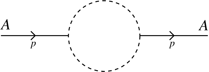
The parity anomaly can also be understood perturbatively. Consider the effective action for the gauge field which is obtained when the matter multiplets are integrated-out with large real masses . Through the one-loop Feynman diagram with non-zero external momentum in Figure 1, the fermions in the matter multiplets generate an effective Chern-Simons interaction99 9 The cubic term in the Chern-Simons action arises from a similar one-loop diagram with three external gauge fields at zero momentum. at level
| (1.11) |
Here is the bare Chern-Simons level in the classical Lagrangian before the matter multiplets are integrated-out. Quantization of means that any corrections to can only arise at one-loop order, and the quadratic Casimir is associated to the pair of vertices in the one-loop diagram.
Note that the shift in depends upon the sign, but not the magnitude, of each real mass parameter .1010 10 The sign of the real mass determines the sign of the fermion mass term. The corresponding mass term for the scalar field in the chiral multiplet is always positive, and both positive and negative values for are perfectly sensible. The overall minus sign in (1.11) is the result of a delicate computation, first performed for adjoint matter in [64]. As a check, for a complex adjoint fermion with positive real mass , the effective Chern-Simons level is according to (1.11). This shift by is twice the shift for a Majorana fermion in the adjoint representation, determined by geometric quantization in [97].
The relation between the bare and effective Chern-Simons levels in (1.11) refines the anomaly-cancellation condition on in (1.10). As usual, gauge-invariance of the effective Chern-Simons action requires to be an integer. If is odd, the same is true for the signed sum on the right in (1.11), so must be a half-integer to ensure the integrality of .
For , a similar version of (1.11) holds,
| (1.12) |
where the quadratic Casimir is replaced by the square of the charge . Again, is half-integral and parity broken when the sum of charges is odd.
The parity anomaly is a fundamental feature of gauge theory in three dimensions, and it is worth understanding in multiple ways.
As a warmup, we explain in Section 2 how the formulas for in (1.11) and (1.12) can be obtained from the exact expression for the partition function in (1.4). Not surprisingly, since the shift in arises by integrating-out charged matter at one-loop, the shift is hidden in the asymptotic behavior of the double-sine function in the integrand of . What is slightly surprising is that has the correct asymptotic behavior to reproduce not only the dependence of on the quadratic Casimir , but also the dependence on the sign of the real mass . Any dependence on the sign of cannot be holomorphic, so agreement with (1.11) relies on a peculiar, though well-known, property of the function .
Holomorphic Factorization.
The parity anomaly is also related to a kind of holomorphic/anti-holomorphic factorization for in its dependence on the real squashing parameter . Factorization was first observed by Pasquetti [82] in the special case and has since been studied in other examples [31, 55, 56, 78, 79, 91], typically with gauge group or and fundamental or anti-fundamental matter. See [17, 21, 30, 43] for several theoretical perspectives on the factorization.
Let us state the basic factorization conjecture, due to the authors of [17]. Introduce parameters
| (1.13) |
as well as
| (1.14) |
For , and define points on the unit circle in the complex plane. Precisely for rational , and are roots of unity. Similarly for , and are valued in the positive corner .
More generally, depends analytically on the pair , so and can be allowed to take complex values. The parameters are then complementary in the following sense. When lies in the upper half-plane, takes values inside the unit disc, and takes values outside the unit disc. Conversely for , the roles of and are reversed. Trivially, the pairs and are swapped under the inversion .
Factorization amounts to the claim that the partition function can be rewritten as a finite sum of products1111 11 Sometimes ‘holomorphic factorization’ refers more literally to the situation in which a sum such as (1.15) has only a single term. We prefer the more expansive notion, relevant when the partition function is the norm-square of a holomorphic section of a higher-rank, hermitian vector bundle.
| (1.15) |
if obeys the anomaly-cancellation condition in (1.10). Here take values in a finite index set , which depends upon the gauge theory data . In general, and also depend upon this data, with only the dependence on the squashing parameter indicated explicitly. Thus is independent of , and depends on as a convergent -hypergeometric series in the variables ; likewise for . Invariance of under implies that is symmetric in the indices .
The formula for in (1.15) resembles the conformal-block decomposition for the partition function of a two-dimensional rational conformal field theory. Following [17], we refer to the functions as the “blocks” of the gauge theory. As emphasized in [17] and as we review in Section 2.2, the block decomposition of is subtle, since both and have a natural boundary of holomorphy on the unit circle . Though is well-defined for these values of and , the blocks themselves are only defined for values and , or vice versa. Nonetheless, from the analytical perspective, the block decomposition in (1.15) provides a very concrete, precise conjecture about the structure of the matrix integral in (1.4).
In this paper, our purpose is to verify the factorization conjecture directly for general gauge groups and weight-multiplicity-free representations . Along the way, we derive explicit expressions for the blocks in low rank, eg. when , , , , and , and for various matter representations.
Most attempts to establish the block decomposition rely upon the holomorphy of the integrand in (1.4) and the residue theorem.1212 12 But see [35] for a very elegant, TQFT-style proof of the block decomposition for rational . Our proof will be no different, though we will use the multi-dimensional residue theorem to streamline computations. Textbook discussions of the multi-dimensional residue theorem appear in [50, 93], and our workhorse version of the residue theorem is proven in [83, 94]. In Section 5 we provide an independent, physically-motivated derivation of the latter theorem using finite-dimensional Grassmann integration, extending the ideas in [14]. A very similar application of higher-dimensional residues to the evaluation of a sigma model partition function has appeared in [48].
The main technical advance in our work is not the use of the multi-dimensional residue theorem per se. Rather, it is to provide a correct justification for the use of the residue theorem at all. As emphasized very clearly in [21], and as we review in Section 3, the standard contour manipulations used to reduce the evaluation of to a residue calculation are valid only in the special case of “maximally chiral” Chern-Simons-matter theories, which have sufficiently small bounded in terms of .1313 13 Eg. if and is the direct sum of copies of the fundamental and copies of the anti-fundamental representation, the “maximally chiral” condition is . This bound on is very restrictive and incompatible with the classical limit . Otherwise when is large, the classical Gaussian factor in the first line of (1.4) simply obstructs the usual step of closing the integration contour for in the upper or the lower half-plane to apply the residue theorem.
To avoid this problem, we play a familiar field theory trick: very massive chiral matter can be integrated both out and in. According to the formula in (1.11), a Chern-Simons-matter theory at level with representation is equivalent to another Chern-Simons-matter theory at level with representation . Here is any representation satisfying , and we eventually take the associated real mass to decouple all effects of the extra chiral matter beyond the one-loop shift from to . By integrating-in auxiliary chiral multiplets and performing a judicious swap of limits, we reduce the general Chern-Simons-matter theory to the “maximally chiral” case, for which the elementary residue calculus applies to the matrix integral in (1.4).
That said, though the idea for our trick comes directly from quantum field theory, we work exclusively with well-defined, finite-dimensional integrals throughout.
The Plan of the Paper.
We begin in Section 2 by reviewing the definition and analytic properties of the double-sine function . As a small application, we use these results in combination with the exact formula for to rederive the one-loop shift (1.11) of the Chern-Simons level, which in turn implies the parity anomaly. Our derivation is probably more useful when run in the opposite direction, insofar as the parity anomaly provides the raison d’etre for an otherwise unusual feature of the double-sine function.
Next in Section 3, we explain where naive attempts to use the residue theorem to prove the factorization conjecture fail. We illustrate the main difficulty in the elementary case .
In Section 4, we show how to salvage the residue calculus by integrating-in massive chiral matter to reduce to level . In this degenerate situation, convergence of the localization integral (1.4) over the Cartan subalgebra is delicate. We provide criteria in Section 4.3 under which the integral converges when the Chern-Simons level vanishes. In Section 4.4 we examine the convergence criteria for supersymmetric QCD with gauge groups of type SU, Sp, and SO. We find that the integral in (1.4) diverges precisely when supersymmetry is spontaneously-broken in the same theory on . We do not have a theoretical explanation for this coincidence, but it seems worthy of further investigation.
In Section 5 we prove a general version of the multi-dimensional residue theorem for complex manifolds with boundary. This theorem interpolates between the Cauchy residue formula and the celebrated Bott residue formula [24]. The proof is based upon the finite-dimensional supersymmetric integral in [14], but that integral must be modified to preserve supersymmetry when the boundary is non-empty. We deduce further consequences when admits a ‘polyhedral decomposition,’ a geometric notion introduced here implying a certain stratification of by CR-submanifolds. The canonical example occurs when is analytically isomorphic to a product of Riemann surfaces, with for each . When each factor is a disk and the integrand admits a suitable meromorphic structure, the result is a sum of Jeffrey-Kirwan [62] residues. In Section 5.4 we illustrate combinatoric features of the multi-dimensional residue theorem with elementary examples.
Finally in Section 6, we combine the technical results in Sections 4 and 5 to demonstrate holomorphic factorization for . This result relies upon the existence of a suitable configuration of ‘Jordan divisors’ in , and much of our work in Section 6 is devoted to producing these divisors. Along the way, in Section 6.2 we discuss some general features of Jeffrey-Kirwan residues, and in Section 6.4 we perform explicit computations of the blocks for the rank-two gauge groups , , , , as well as , with various matter representations. Some of our formulas have appeared previously in the literature, but others are new.
The paper includes three appendices.
In Appendix A, we record our Lie algebra conventions, including the normalization convention for the quadratic Casimir so that the one-loop formula in (1.11) holds universally.
In Appendix B, we prove an elementary lemma about hyperplane arrangements and convex polytopes. This lemma is used in the discussion in Section 6.2 of Jordan divisors for gauge groups with rank larger than two.
In Appendix C, we discuss the asymptotics under analytic continuation in for torus knot observables in Chern-Simons-matter theories. Though not directly related to the parity anomaly or holomorphic factorization, this material fits broadly with our theme and is perhaps useful to include. Surprisingly, at least for torus knots, the chiral matter does not change the qualitative behavior deduced for the colored Jones polynomial in [53, 54, 77].
Acknowledgments.
First and foremost, we thank Tudor Dimofte for his comments and suggestions on a draft version of this paper. We further thank Cyril Closset, Thomas Dumitrescu, and Valerio Toledano Laredo for helpful conversations. CB additionally thanks the organizers and participants of the 2016 Simons Summer Workshop, hosted at the Simons Center for Geometry and Physics, Stony Brook University, where some of this work was performed. Portions of the paper were also written while CB was a visitor at Harvard University and at the Perimeter Institute for Theoretical Physics. CB thanks the members and staff of both institutions for their generous hospitality during those visits.
This paper contains results which appear originally in the PhD thesis [10] of NB.
The work of CB is supported in part under National Science Foundation Grant No. PHY-1620637. Any opinions, findings, and conclusions or recommendations expressed in this material are those of the authors and do not necessarily reflect the views of the National Science Foundation.
2 Parity Anomaly From Double-Sine
We begin in Sections 2.1 and 2.2 by reviewing the definition and properties of the double-sine function . The essential notion goes back over a century to Barnes [12, 13], with more recent revivals in [40, 69, 70, 90]. For additional discussion about the double-sine, see for instance the relevant portions of [26, 27]. A complete review appears in [71].
In Section 2.3, we combine these properties of with the exact formula for to rederive the one-loop renormalization of the Chern-Simons level in (1.11). This feature of is well-known to experts and for unitary gauge groups has been previously observed in [5, 20, 95].
2.1 Definition of the Double-Sine Function
The double-sine function admits a variety of analytic expressions which could be used as a definition. We will begin with the expression which appears naturally in the localization computation leading to (1.4),
| (2.1) |
Because the double-sine arises from a one-loop determinant, is expressed as an infinite product over a pair of positive integers . This infinite product does not converge for any value of and hence is only a formal expression. We emphasize this fact by using the symbol ‘’ in (2.1) rather than an equality.
The true meaning of the product formula in (2.1) is that will be defined as a meromorphic function of with zeroes and poles at the locations below,
| (2.2) | ||||
See Figure 2 for a sketch. For real, all zeroes of lie along the positive imaginary axis, and all poles lie along the negative imaginary axis, including the origin. For irrational , the zeroes and poles are moreover simple. Otherwise, if is rational, each zero or pole at has the same multiplicity as the number of positive integral pairs satisfying the relations in (2.2). Later in Sections 3 and 4, we assume the generic case precisely to avoid thorny arithmetic associated to higher-order poles in .
Once the zeroes and poles are fixed, is determined up to multiplication by a non-vanishing entire function of . Equivalently, will be determined once its asymptotic behavior as is fixed. From either perspective, to define honestly as a meromorphic function, the infinite product in (2.1) must be regularized.
We consider the logarithm, again a formal expression,
| (2.3) |
In logarithmic form, the divergence of the sum over and on the right in (2.3) is clear. To obtain an absolutely-convergent series, we differentiate the summand successively with respect to , so that
| (2.4) |
and
| (2.5) | ||||
In passing to the second line of (2.5), we just evaluate the difference in the first line. Evidently, the series for the would-be second-derivative of does converge absolutely and uniformly on compact subsets of , since the denominator in the summand grows quartically for large and fixed , while the numerator only grows linearly.
Although the formal product formula in (2.1) does not actually define , the convergent series in (2.5) does define the second-derivative of . Thus
| (2.6) |
where and are undetermined constants, possibly depending upon , and is obtained by integrating the holomorphic function in (2.5) twice with respect to .1414 14 For instance, the integration can be accomplished by using the Taylor expansion of the series in (2.5) about a specified point in the -plane. The choice of the point is absorbed into the constants and . Note that satisfies
| (2.7) |
as the series in (2.5) is manifestly invariant under the inversion . If and are themselves invariant under , the double-sine obeys
| (2.8) |
The constants and describe potentially -dependent renormalizations of the partition function on , in the sense that any choices for these constants can be absorbed into the definitions of other constants already appearing in our formula for . From (1.4) and (1.5), the constant can be absorbed into the overall normalization of , and the constant can be absorbed into the definition of the abelian FI parameter . When is non-abelian and simple, no FI term is present, and simply cancels out in the product over weights of in (1.4).
The values of the constants and can be fixed in various ways. The standard approach is to use the Barnes double-zeta function
| (2.9) |
depending on non-zero parameters . For sufficiently large, the sum on the right is absolutely-convergent for all values of . Otherwise, the definition of is extended to other values of by analytic continuation, with simple poles at .
The Barnes double-zeta function is a generalization of the classical Hurwitz zeta function
| (2.10) |
Specifically, by analogy to (2.9) set
| (2.11) |
Then immediately,
| (2.12) |
For later reference, recall also the Hurwitz zeta identity
| (2.13) |
With the Barnes double-zeta function, we next introduce the Barnes double-gamma function1515 15 Our normalization of follows the modern convention, which differs from that of Barnes.
| (2.14) | ||||
As suggested by the formal product representation in the second line of (2.14), is a non-vanishing meromorphic function of with poles at the locations
| (2.15) |
If the ratio is irrational, each pole is simple. Otherwise, the poles have the multiplicities given by the product formula.
The definition (2.14) of the double-gamma function should be compared to the Lerch formula for the classical Euler gamma function
| (2.16) |
written in terms of the Hurwitz zeta. To make the comparison precise, let us introduce
| (2.17) |
From (2.12) and (2.17), we see that is related to the classical gamma function by an elementary multiplicative factor,
| (2.18) |
In passing to the second equality, we apply the Hurwitz zeta identity in (2.13).
Comparing the product formulas in (2.1) and (2.14), the double-sine function can now be defined as the ratio of double-gamma functions
| definition | (2.19) |
With this definition, is meromorphic with zeroes and poles at the correct locations (2.2) and with the correct multiplicities. Implicitly, the formula in (2.19) specifies a choice for the renormalization constants and in (2.6).
The double-sine is manifestly symmetric under the exchange of and as in (2.8). Also under inversion of ,
| inversion | (2.20) |
Trivially from the definition (2.19), we have the special value
| (2.21) |
Before proceeding, let us mention one reason for the name ‘double-sine’. By comparison to (2.19),
| (2.22) | ||||
Here we use the relation of to the Euler gamma function in (2.18), along with the reflection formula
| (2.23) |
The quotient of double-gamma functions in the definition of serves as the proper generalization of the single-gamma reflection identity (2.22) in which an ordinary sine enters.
Alternative Definitions.
Many cousins to the double-sine function also appear in the literature, so the reader must take care with conventions. Among popular variants, the non-compact quantum dilogarithm [41] is related to by
| (2.24) |
The -function of Ruijsenaars [87] is related by
| (2.25) |
The hyperbolic gamma function of van de Bult [26] is related by
| (2.26) |
Finally, the function considered in [27] is related by
| (2.27) |
2.2 Properties of the Double-Sine Function
We require two further properties of . The first property concerns the value of the residue at each pole (2.2) along the negative imaginary axis. The second property concerns the asymptotic behavior as . Both properties will be essential for our analysis of the partition function .
Quasi-periods and Residues.
We return to the Barnes double-zeta function in (2.9). Trivially, by rearranging terms in its defining sum, the Barnes double-zeta function obeys
| (2.28) | ||||
Taking derivatives with respect to in (2.28), we find that the double-gamma function in (2.14) satisfies the multiplicative relation
| (2.29) | ||||
The definition of in (2.19), along with the reflection formula in (2.22), then implies the quasi-periodic transformation
| quasi-periods | (2.30) |
By applying the quasi-periodic transformations in succession, we deduce
| (2.31) | ||||
For the sign in the first line of (2.31), note that . Combining the expression for in (2.31) with the inversion formula in (2.20), we obtain a product formula
| (2.32) |
The function has a simple pole at with residue and hence a Laurent expansion
| (2.33) |
The leading singularity at on the right in (2.32) then determines
| (2.34) |
The sign of the residue apparently requires more effort to fix, so we just quote the literature:
| (2.35) |
The quasi-periods in (2.30) then imply the special values
| special values | (2.36) |
The quasi-periodic transformations in (2.31) can be iterated to evaluate the residue of at any other pole. By a small computation, for each ,
| (2.37) | ||||
Alternatively, when the relation in (2.37) is read backwards,
| (2.38) | ||||
From (2.35) and (2.38), the residue of at each pole on the imaginary axis is then
| (2.39) |
Note that the product on the right in (2.39) is finite for all so long as is irrational, meaning the poles of are simple. Otherwise, the product diverges at the special poles of with higher degree, due to the vanishing of or for appropriate .
-Pochhammer Symbols.
Both the quasi-periodicity relation in (2.37) and the residue formula in (2.39) are frequently rewritten in the language of -Pochhammer symbols. This notation is useful for emphasizing the algebraic as opposed to analytic properties of the double-sine function, so we briefly recall it.
Given an integer , define the polynomial
| (2.40) |
By convention , and an important special case will be
| (2.41) |
The finite product in (2.40) can be extended to an infinite product
| (2.42) |
which converges to a holomorphic function of when . Thus can be rewritten as the quotient
| (2.43) |
This expression for also makes sense for negative values of , so we set
| (2.44) | ||||
For example,
| (2.45) |
As their essential feature, both the positive and the negative -Pochhammer symbols for finite are rational functions of .
With some rearrangement of factors in (2.44), the negative -Pochhammer symbol can be alternatively recast
| (2.46) |
Also worth remarking for its modular behavior, the infinite Pochhammer symbol is directly related to the Dedekind eta-function
| (2.47) |
In the language of -Pochhammer symbols, the quasi-periodicity formula (2.37) becomes more succinctly
| (2.48) | ||||
where we recall the identifications
| (2.49) |
We omit the derivation of the formula in (2.48), which follows from the identity , the definition of the -Pochhammer symbol, and elementary algebraic manipulations.
Beyond its brevity, the -Pochhammer expression for the double-sine function has two virtues. In the preceding quasi-periodicity formulas (2.37) and (2.38), the integers and are both assumed positive, as the behavior of depends upon whether shifts up or down the imaginary axis. By contrast, the -Pochhammer formula in (2.48) reproduces not only (2.37) but also (2.38), after the naive reflection . Hence the -Pochhammer expression in (2.48) is correct for both positive and negative values of . Moreover, we already see from (2.48) the beginning of the desired holomorphic factorization for .
Reflecting and taking the limit in (2.48), we obtain a -Pochhammer formula for the residues of the double-sine function,
| (2.50) | ||||
By the -Pochhammer identity in (2.46) with , the residue can be rewritten in the slightly more transparent fashion below,
| (2.51) |
Expressing and in terms of products of sines, one can readily check that the result in (2.51) reproduces the previous version (2.39) of the residue formula. According to (2.51), each residue of is a rational function of and , with poles at roots of unity in the complex - (resp. -) plane.1616 16 Recall that and lie on the unit circle precisely when is real. As mentioned earlier, the higher-order poles in occur for rational values of , for which and are roots of unity. The -Pochhammer residue formula will be our workhorse in the analysis of holomorphic factorization.
Integral Representation and Asymptotics.
To apply the residue calculus to the partition function in (1.4), we require information not only about the poles and residues of but also about the asymptotic behavior as . The latter knowledge is crucial for understanding which contour manipulations of the matrix integral are allowed.
The asymptotic behavior of for large is most easily deduced from yet another representation of the double-sine function, this time in terms of the integral
| (2.52) | ||||
The integral formula for is originally due to Ruijsenaars [87] and is reviewed in Chapter 2 of [26], where the reader can find a proof of (2.52).1717 17 Again, neither the conventions in [26] nor [87] agree precisely with ours, so some translation is required to read these works.
Let us discuss the domain of parameters in which the integral representation for is valid. The variable runs over the positive half-line , so the expression in (2.52) must be integrable near both and . For , the integrand behaves to leading-order like (the poles of the respective terms in parentheses cancel), so integrability near is assured. Otherwise, if we require the second term in the argument of (2.52) to decay exponentially as , the imaginary part of must be bounded above and below by . Precisely within this strip depicted in Figure 3, is both regular and non-vanishing, consistent with the presentation in (2.52).
The asymptotics of become clearer after some manipulation of the integral
| (2.53) |
Because the integrand is an even function of , the integration domain can be unfolded to the real-line and written more symmetrically as the principal-value integral
| (2.54) |
As usual,
| (2.55) |
To simplify still further, consider the contour denoted by in Figure 4. This contour includes a small semi-circular detour of radius around the origin in the upper half-plane. If a meromorphic function is symmetrically-integrable about the origin, meaning that the Laurent expansion of has singular terms1818 18 Eg. . with exclusively odd degree in , then
| (2.56) |
Here the contribution from the small semi-circle in Figure 4 has been added and subtracted to the right-side of (2.56) in the limit . When applied to the formula for in (2.54), we obtain
| (2.57) |
By shrinking the contour at infinity, we note that for the second term in (2.54).

With the new expression (2.57) for , the double-sine function can be presented more conveniently in terms of the contour integral
| (2.58) | ||||
again valid within the strip . We assume that is generic, so that the integrand in (2.58) has simple poles along the imaginary axis at or for integer , along with a triple pole at .
The asymptotic behavior of for now depends upon whether the real part of is positive or negative. If , the integral over in (2.58) can be evaluated by closing the contour in the upper half of the -plane and applying the residue theorem. After a small calculation,
| (2.59) | ||||
Therefore in terms of the parameters and , the argument of the exponential in (2.58) has the series expansion
| (2.60) | ||||
When the real part of is negative, the contour in (2.59) must be closed in the lower half of the -plane. From Figure 4, we see that the pole at also contributes to the residue computation in this case,
| (2.61) | ||||
The quadratic expression on the first line of (2.61) is the contribution from the pole at . Hence in contrast to (2.60),
| (2.62) | ||||
The expressions in (2.60) and (2.62) are exact for in the strip , so we deduce the asymptotic behavior
| (2.63) | ||||
up to exponentially-small, -contributions from the respective series in (2.60) and (2.62). This result is worthy of several remarks.
- 1.
The asymptotic behavior of as depends upon the sign of the real part of and is not analytic in . Even for an entire function such as , the asymptotic expansion as may jump between sectors in the complex -plane. The non-analytic behavior in (2.63) will ultimately be responsible for the non-analytic dependence on the sign of the real mass in the one-loop formula (1.11) for the effective Chern-Simons level .
- 2.
The definition of in (2.19) amounts to a specific choice for the constants and in (2.6). With some other choice, the double-sine function is renormalized as
(2.64) Comparing to (2.63), we see that the leading, quadratic dependence on in the argument of the exponential is determined independently of the choice for and , whereas the subleading asymptotic behavior of depends on the renormalization scheme.
- 3.
The double-sine function grows or decays very rapidly as , at the rate of the Gaussian . Here we model the Gaussian, including the ‘’, on the effective Chern-Simons term in the matrix integral (1.5). However, the sectors of asymptotic growth vs. decay differ sharply between the Gaussian and the double-sine, due to the non-analytic behavior in (2.63). As illustrated in Figure 5, the classical Gaussian vanishes when in the first and third quadrants of the complex plane. By contrast, vanishes when in the lower half-plane. In the complements to these regions, the Gaussian and the double-sine respectively diverge as .
- Decomposition.
The respective series expansions for in (2.60) and (2.62) imply a factorization in the dependence on of the sort required for the factorization of in (1.15).
For later use in Sections 3 and 4, we introduce a decomposition of the double-sine with argument
| (2.65) |
where
| (2.66) |
By the quasi-periodicity relation in (2.48),
| (2.67) | ||||
All dependence on the integers and is absorbed by the prefactors in the first three lines of (2.67). Clearly, and enter each factor separately, so these terms are consistent with the - decomposition.
Otherwise, since lie in the unit interval, the series expansions in (2.60) and (2.62) apply to the final term in (2.67). For , a brief calculation shows
| (2.68) | ||||
We omit the similar expansion for , which only differs by a few signs. Again, all dependence on and factorizes.
Fix a parameter with , and let as above. The preceding expansion of can be simplified further via the identity
| (2.69) |
This identity is elementary, but it illustrates that has an interesting feature as a holomorphic function of .
In the first case , we apply the Taylor expansion of about and then reorder the absolutely-convergent series to obtain the sum of logarithms in (2.69). In the second case , we rewrite and expand similarly around . Otherwise, has poles densely distributed at all roots of unity on the circle , so the function is not continuous there. For the same reason, cannot be continued analytically from the region to , as more or less apparent from (2.69). In the terminology of the classic analysis text [49] (see especially Ch. IV, §87), the circle is a “natural boundary” for . Depending upon the magnitude of , the series in (2.69) effectively represents a pair of distinct holomorphic functions.
Since enters the expansion (2.68), the holomorphic functions involved in the - decomposition of the double-sine also possess natural boundaries on the unit circle in the complex -plane, shown in Figure 6. This circle corresponds to physical values for the squashing parameter under the identifications and . Hence the analytic - decomposition for only becomes sensible when is continued to complex values, and the result depends upon whether and , or and . We emphasize that itself is perfectly well-defined for (as we have assumed so far). The existence of the natural boundary plays an important role in [17], to which we refer the reader for a more thorough discussion of the physical interpretation.
For the region and , the identity (2.69) applied to the expansion (2.68) implies a convergent product formula for the double-sine,
| (2.70) | ||||
Alternatively for and , the numerator and denominator swap,
| (2.71) | ||||
Both infinite products are conveniently summarized by -Pochhammer symbols (2.40), eg.
| (2.72) |
The product formula (2.71) for the double-sine applies when lie in the unit interval, but this result can be immediately continued for all via (2.67). We present the complete result for the - decomposition
| (2.73) |
where we set1919 19 The notation in (2.73) is imprecise, as the functions on the right depend not just on the value of but also on the way of writing the imaginary part of as the sum in (2.74). Nonetheless, we use this shorthand to avoid further cluttering the notation.
| (2.74) |
The phase does not depend upon the squashing parameter ,
| (2.75) |
while does, both explicitly and implicitly through ,
| (2.76) | ||||
The superscript ‘’ indicates that is defined only for positive. Like the function in (2.69), is an analytic function of for both and , but does not depend continuously on across the natural boundary . Dually,
| (2.77) | ||||
The function and its sibling are very beautiful. As a consequence of the -binomial theorem, both are -hypergeometric series. We omit a review of the latter topic, as it will not be important here. Also, when evaluated at the special points and for the double-sine, both functions are directly related to the classical eta-function. For instance,
| (2.78) |
and
| (2.79) |
including the tell-tale .
A Toy Model of Factorization.
Before proceeding, let us briefly illustrate how the - decompositions in (2.73) and (2.80) induce a factorization for associated integrals of the double-sine . We begin with a non-example, in which the factorization is obstructed, and then present the most basic example.
For the non-example, we consider the integral of the double-sine function over the real line,
| (2.83) |
The parameter here plays the role of the real mass parameter in (1.4), and indicates the upper-half of the complex plane. We assume that has a positive imaginary part so that no poles of the integrand lie on the real axis. Recall from Figure 2 that otherwise has a pole at . Of course, the real part of can be absorbed into a shift of the integration variable in (2.83). Since varies holomorphically with , must then be independent of for values in .
As indicated in Figure 5, the double-sine function decays rapidly as goes to infinity in the lower half-plane. Hence can be evaluated via the residue theorem once the real integration contour is closed as in Figure 7. According to (2.2), the integrand of (2.83) has poles at locations
| (2.84) |
For generic , every pole is simple and lies in the lower half-plane. The residue of at each pole is given by the expression in (2.51). Hence
| (2.85) | ||||
Here the dependence on has been subsumed into a dependence on and . The double sum over integers in the second line of (2.85) nearly factorizes into a product of separate - and -series given by the terms in brackets, but this factorization is obstructed by the oscillating phase .
To eliminate the troublesome phase, we replace the integrand in (2.83) by a pair of double-sine functions,
| (2.86) |
By fiat, we choose the signs in (2.86) so that the integrand is invariant under the reflection . The dependence on can no longer be eliminated by a simple shift, so will now be a non-trivial holomorphic function of . The coefficient of for merely serves to simplify later formulas and could be eliminated by a rescaling of . As will be clear in Section 3.2, the integrand mimics the structure of the one-loop determinant for massive chiral matter in a single copy of the fundamental representation of . The inversion is there interpreted as the residual Weyl symmetry on the Coulomb branch.
To apply the residue calculus to , we first consider the analytic structure of the product of double-sines in (2.86). Evidently from (2.63), the leading Gaussian terms in each factor cancel as , so that in either half-plane
| (2.87) |
Provided the combination is real and positive, as true when is real and positive and is purely imaginary and small, the result in (2.87) decays exponentially along rays in both the left and the right half-planes. We assume the reality condition in order to apply the residue calculus to ; later we analytically continue the result to other values of the parameters and .
Due to the relative sign in the arguments of the double-sines, the product in (2.87) has simple poles extending symmetrically upwards and downwards in the imaginary direction,
| (2.88) |
The analytic structure of the integrand in (2.86) thus resembles that of the function , and can be evaluated as a sum of residues by closing the integration contour in either the lower or the upper half-plane. For convenience, we close the contour in the lower half-plane, as shown in Figure 8.
The residue calculus now implies
| (2.89) | ||||
where we again use the formula (2.51) for the residues of the double-sine at each simple pole. The - decomposition of the double-sine in (2.73) and (2.80) provides a further factorization of the term in the summand. Upon analytic continuation, the - decomposition depends upon the sign of the real part of as well as the norm of . For instance, if and , then concretely2020 20 Recall that implies the complementary bound when both and are expressed in terms of the squashing parameter .
| (2.90) | ||||
Upon substituting the respective definitions in (2.76) and (2.77) for and , we rewrite
| (2.91) | ||||
Because the phase enters both the residue (2.89) and the - decomposition (2.91) of the double-sine, the obstruction to holomorphic factorization of vanishes.
From the expressions in (2.89) and (2.91), we see that is given by a product
| (2.92) |
where we introduce the fugacity variables
| (2.93) |
The holomorphic ‘blocks’ and in this example then admit expansions
| (2.94) | ||||
These formulas for and can be simplified by elementary manipulations which follow from the definition of the -Pochhammer symbol in (2.40). After a small amount of algebra,
| (2.95) | ||||
For fixed and , the series in (2.95) are convergent for sufficiently small and sufficiently large. See Figure 9 for a numerical plot of for values of and . In other regions of the parameter space, eg. and , the integral factorizes in the same fashion, but with different functions appearing as the holomorphic blocks.2121 21 Due to the denominator in the series expansion (2.95) for , the block has a natural boundary of holomorphy on the unit circle , and similarly for .
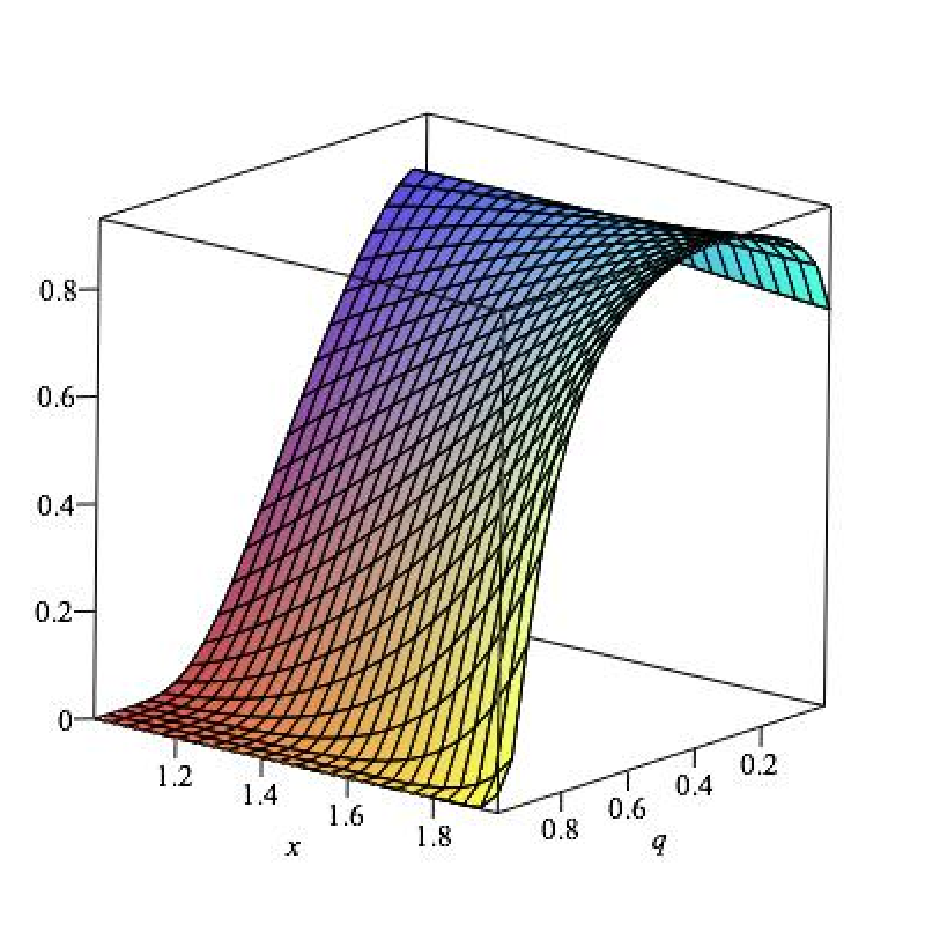
The integral thus has exactly the structure conjectured for the partition function in (1.15), for the trivial index set of one element. All dependence on the parameter can be factored into analytic dependence on the pairs and in the respective holomorphic blocks and . As the non-example involving shows, the existence of such a factorization is a non-trivial statement about the function .
2.3 One-Loop Shift in the Chern-Simons Level
We return to the exact formula for the Chern-Simons-matter partition function
| (2.96) | ||||
From the formula in (2.96) and the analytic properties of the double-sine reviewed in Section 2.2, we now rederive the classic shift in the Chern-Simons level when chiral multiplets in the representation are integrated-out with large real masses , ie.2222 22 We implicitly assume along the real axis. Else when is complexified, should be replaced by the sign of the real part .
| (2.97) |
For with charges , the formula for is to be interpreted as
| (2.98) |
As we discussed in Section 1, the global parity anomaly can be understood macroscopically from the shift in (2.97) or (2.98) and the integrality condition . See for instance § in [5] for a previous analysis of in the massive limit.
To ensure that the limit is well-defined, we must renormalize other parameters in (2.96) beyond the level . As we will see momentarily, must be allowed to depend on the real masses via
| (2.99) |
Here is the dimension of the irreducible representation , and the finite, -dependent terms in (2.99) appear by convention. If , the FI parameter appearing in (1.5) must also diverge linearly with ,
| (2.100) |
The choice of finite part in (2.100) defines the effective FI parameter in the low-energy gauge theory without matter. Like all one-loop matching relations, the relation between and depends upon the renormalization scheme, fixed here implicitly through definition (2.19) of the double-sine function.
Finally, observe that the renormalization of the FI parameter depends upon the charges , the real masses , and the metric parameter . Quantum corrections to the FI parameter in three dimensions cannot depend upon holomorphic quantities such as couplings in the superpotential, but dependence upon the real parameters is allowed. Both renormalizations in (2.99) and (2.100) of course respect the inversion . As explained in [32, 33], the term quadratic in which enters is related to a (possibly fractional) Chern-Simons term for the background gauge field associated to the given real mass; our renormalization scheme amounts to subtraction of background Chern-Simons terms.
Because the formula for is exact for all parameter values, integrating-out massive chiral matter just means taking the limit in (2.96). In this limit the asymptotic expansion (2.63) for the double-sine is applicable, so
| (2.101) | ||||
The dependence on captures both asymptotic behaviors for in (2.63). The one-loop contribution to the matrix integrand from massive chiral matter in the irreducible representation becomes
| (2.102) | ||||
Here denotes the finite set of weights for the representation , with cardinality . When the gauge group is simple, the sum over weights in vanishes, so
| (2.103) |
Also,
| (2.104) |
where is the quadratic Casimir of the representation. The sum over weights on the left in (2.104) is invariant under the action of the Weyl group on , so it must be proportional to the quadratic form .2323 23 By convention, is positive, consistent with the manifest positivity on the left in (2.104). See (A.34) in Appendix A for a small proof that is precisely the constant of proportionality.
For the special case with charges , the limit in (2.102) is replaced by the corresponding
| (2.105) | ||||
Of the terms in the limiting expansion above for , only the term proportional to will be important. After we substitute the expansion for into the matrix integral (2.96), the renormalization of in (2.99) serves to cancel the -independent terms in (2.102) and (2.105). For the term which is linear in , the renormalization (2.100) of the FI parameter ensures that in (1.5) only depends upon the effective parameter in the limit . Both renormalizations are consistent with the underlying ambiguity (2.64) in the definition of .
Finally, the terms with quadratic dependence on in (2.102) and (2.105) can be absorbed by a finite shift of the bare Chern-Simons level in the original matrix integral (2.96), so that
| (2.106) | ||||
In this form, the limiting matrix integral describes the partition function of pure Chern-Simons theory, with gauge group and without matter, at level . The coefficient of in (2.102), in combination with the Lie algebra relation in (2.104), leads precisely to the formula for in (2.97). The abelian case (2.98) follows identically.
Further Remarks.
Our derivation of effective level from the exact formula for is nice but hardly unexpected. The finite shift in the Chern-Simons level is famously determined at one-loop order [85, 86] in perturbation theory, and the double-sine factor in (2.96) also arises from a semiclassical, one-loop computation.
Yet the derivation does resolve a small paradox concerning the analytic behavior of the double-sine function itself. As claimed in (2.63) on the basis of its integral representation, grows like a Gaussian as . This growth means that one-loop fluctuations of the chiral matter multiplet contribute to the matrix integral in (2.96) with the same asymptotic magnitude as the classical Chern-Simons action for the vector multiplet. The reader might well be uneasy to hear that a quantum effect competes in magnitude with a classical effect even far along the Coulomb-branch .2424 24 By contrast, the one-loop contribution from the vector multiplet, given by the product of hyperbolic sines in the second line of (2.96), is naturally subleading for large once the integration contour for is rotated slightly away from the real axis. In this light, the claimed asymptotics for demand a physical explanation.
Our derivation of the formula in (2.97) reveals that the unusual asymptotics of in (2.63) are not only correct, but are required by the parity anomaly. Even the peculiar asymptotic dependence on the sign of is necessary to recover the corresponding physical dependence of on the sign of each real mass . For the same reason, the discrepancy between sectors of convergence in Figure 5 must be an honest feature of the double-sine function, with consequences for the residue calculus.
3 Factorization and Obstruction in Rank-One
As preparation to our analysis of the factorization conjecture (1.15) for general gauge groups and matter representations , we revisit the abelian case originally discussed by Pasquetti [82]. Beyond reviewing the mechanics of factorization in an elementary example, we wish to highlight an important subtlety when the Chern-Simons level is non-vanishing. Later in Section 3.2, we compare to the non-abelian (but still rank one) example .
3.1 SQED at Non-Vanishing Level
Throughout Section 3.1, for are electric charges for chiral matter multiplets minimally coupled to an abelian vector multiplet at Chern-Simons level . Without loss, we take all charges to be non-zero.
The matrix integral for the partition function on then reduces to an integral over ,
| (3.1) |
To guarantee absolute-convergence, we give a small positive imaginary part. We also assume the real mass parameters are non-zero, distinct, and generic. As indicated above, we give each a positive imaginary part to ensure that the integrand avoids the pole of at and is regular everywhere along the real axis. Otherwise, for complex values of , the integrand is a meromorphic function with countably-many simple poles distributed according to Figure 2 and with an essential singularity at infinity.
Chirality Bound.
The residue calculus provides a natural tool to evaluate the integral in (3.1), provided we can pick a suitable closed integration contour . The contour must contain the real line , and the integral over the complement must vanish. The existence of is not guaranteed and depends very much on the asymptotic behavior of the integrand as .
When , the contour exists for generic choices of charges. In this case, the asymptotic behavior of the integrand in (3.1) is dominated entirely by the product of double-sines arising from the chiral matter at one-loop. Via (2.63), as with fixed ,
| (3.2) |
where is the signed sum
| (3.3) |
So long as , the contribution from the FI term in (3.1) is subleading for large and can be ignored. Clearly, if and , the integrand decays exponentially as with , so can be closed in the lower half-plane. Conversely for and , the integrand decays exponentially as with , so can be closed in the upper half-plane. See Figure 10 for a graphical summary of the situation. We review the residue computation [82] with this choice of contour momentarily.
When the Chern-Simons level is non-vanishing, the contour may or may not exist, as the Gaussian term proportional to in (3.1) competes in magnitude with the product (3.2) of double-sines for large . If the Chern-Simons level is not too large, meaning that is bounded by
| chirality bound | (3.4) |
then the contour can be chosen exactly as for the case in Figure 10. But if violates the bound in (3.4), the Gaussian term dominates, and the integrand does not decay consistently over either the upper or the lower half-planes. Compare to (a) in Figure 5. Evidently, if the upper bound on is violated, no choice for exists which is amenable to the residue calculus.
Finally, in the marginal case , the subleading -terms omitted from the expansion in (3.2) become important. With -terms included, the one-loop matter determinant behaves as
| (3.5) |
where
| (3.6) |
Briefly, when is positive, the contour can still be closed in the lower half-plane, provided the FI parameter obeys the auxiliary bounds
| (3.7) |
This condition ensures the decay of the integrand in the quadrant where the Gaussian term is cancelled by the double-sine, meaning and . Conversely when is negative, can be closed in the upper half-plane if
| (3.8) |
ensuring decay of the integrand in the quadrant where and . When either bound on in (3.7) or (3.8) is violated, a suitable contour does not exist.
The bound reflects the fact that the residue calculus is not effective for evaluating integrals which are asymptotically Gaussian. Clearly, the strength of the bound depends upon the magnitude of , which measures the net chirality of the matter representation . For instance, if is a real representation of and so is preserved under the charge conjugation , then . In this case, the residue calculus applies only when , with appropriate range of . Alternatively, when the bound in (3.4) is read backwards for fixed , the residue calculus applies only when the matter spectrum is sufficiently chiral.
One might wonder whether the chirality bound indicates an intrinsic feature of the partition function , such as a failure of factorization in the semiclassical limit , or whether it merely describes a failure in the most naive application of the residue calculus. In Section 4.2, we demonstrate that the second circumstance holds, and the apparent bound on in (3.4) can be evaded with more involved analytic maneuvers.
Residue Calculus for SQED Partition Function.
We now review the residue calculus for in the case that the chirality bound in (3.4) is satisfied. Explicit formulas for are quite complicated in general, so our focus will be on the structure of the result and how this structure depends upon the gauge theory data.
According to (2.2), the product of double-sines in the integrand for has poles on the union of divisors
| (3.9) |
For generic, poles corresponding to different divisors do not coincide, for , and every pole is simple. Also, because we assume , the poles in each are located in either the upper or the lower half-plane, dictated by the sign of the charge .2525 25 Because has a small positive imaginary part, this statement remains true for the special pole with , which is slightly displaced from the real axis. E.g. for , all poles in lie in the lower half-plane.
When is computed as a sum over residues, not every pole in the integrand contributes. As shown in Figure 10, the appropriate integration contour depends upon the sign of in (3.3). If , the contour must be closed in the lower half-plane, so only the divisors associated to positive charges contribute to the sum over residues. Conversely if , only the divisors for negative charges contribute.
We will discuss the residues themselves shortly, but let us first abbreviate
| (3.10) | ||||
Depending on the sign of , the residue calculus implies
| (3.11) |
versus
| (3.12) |
The minus sign in (3.11) accounts for the orientation of the contour in Figure 10, and the respective sums run over the set of charges with the given sign. Of course, when is strictly positive, at least one charge is necessarily positive as well, so the sum over residues is always non-empty!
To suppress the proliferation of signs, we restrict attention to the case , meaning for all terms in the residue sum.
We are left to evaluate the residue itself. We have already determined the residues at poles of in (2.51), and the - decomposition in (2.73) and (2.80) provides a description of at regular points, as soon as we give a small imaginary part. All that remains is careful bookkeeping.
The essential novelty of our result for SQED concerns the arithmetic dependence on the charges. For this reason, we must keep track of the values of the integers in modulo the corresponding charge . We decompose
| (3.13) | ||||
meaning
| (3.14) |
After tedious but trivial algebra, which we spare the reader, we find that each residue in (3.10) can be expressed as a product2626 26 As usual for , .
| (3.15) | ||||
We recall from the Introduction
| (3.16) |
and
| (3.17) |
To account for the FI parameter in SQED, we also introduce variables
| (3.18) |
We provide expressions for , , and below, but let us first emphasize the important properties of (3.15).
Properties of the Residue.
All dependence on the squashing parameter in is captured through the dependence on the variables and , which appear in the respective functions and . The dependence on these variables completely factorizes.
We indicate explicitly the dependence on the integers as well as the congruence classes associated to . The phase depends on neither nor , the function is independent of , and the dual function is independent of . The latter feature can be traced to the same properties of the formulas for and in (2.76) and (2.77).
Because the SQED partition function involves a sum over , we must also consider to what extent the dependence on and factorizes in . The formula in (3.15) displays no nice factorization in terms of the congruence classes modulo . But precisely when the anomaly-cancellation condition is satisfied, so that the phase factor in the first line of (3.15) is trivial, the dependence on the integers and does factorize. The combination appears in (3.15) for the same reason it appeared in Section 2.3, as the coefficient of the leading Gaussian term in the integrand.
The phase is given in terms of the gauge theory data by
| (3.19) | ||||
where denotes the symplectic pairing
| (3.20) |
If , the phase still depends non-trivially on the product through the first term in (3.19). For general values of , factorization in is spoiled by this term.
Formulas for and , even when written in terms of and from Section 2.2, are more involved. In detail,
| (3.21) | ||||
where
| (3.22) |
One can check straightforwardly that does not depend on the integer or the variables . For instance, assuming ,
| (3.23) | ||||
The detailed formulas in (3.21) and (3.23) are not themselves important for the present work. We provide them only to illustrate that such formulas exist. Also, note that can be presented analytically as a convergent product of rational functions in . Finally, does depend on the index through the initial phase factor in (3.21) as well as the phase which enters the final -Pochhammer term in (3.23). This dependence further spoils factorization in the congruence classes modulo .
For completeness (or masochism), we record the parallel formula for ,
| (3.24) | ||||
Factorization at Higher Degree.
From (3.15), the partition function for positive is given by the successive sums
| (3.25) | ||||
where we reduce modulo as in (3.13). Precisely when , the phase in the first line of (3.25) is trivial, so we can rewrite in the factorized form
| (3.26) |
with blocks given by the series
| (3.27) |
Comparing to the Factorization Conjecture in (1.15), we identify the index set for SQED with the set of triples
| (3.28) |
and is the diagonal matrix
| (3.29) |
For , the structure is identical, but with contributions from negative charges.
To summarize, for each chiral multiplet whose charge agrees in sign with , we obtain chiral blocks which are labelled by elements in the group . The simplest case occurs when all chiral matter fields have unit charge for . In this “maximally-chiral” situation, mod , and the residue calculus applies if . Each chiral matter field contributes exactly one chiral block to the partition function, with trivial labels for congruence classes.
For the maximally-chiral theory, the phase in (3.19) becomes an uninteresting constant depending only on the real masses, and the function in (3.21) specializes to
| (3.30) | ||||
with
| (3.31) |
For instance, if (meaning for ) and ,
| (3.32) |
See [82] for a nice interpretation of in terms of a vortex partition function.
3.2 Comparison to Gauge Theory
In marked contrast to , all representations of are self-dual, either real or pseudoreal depending upon whether the spin is integral or half-integral. As we now explain, this fact drastically alters the asymptotic behavior of the matrix integrand, with consequences for the naive residue calculus.
Some Preliminaries.
According to the Lie algebra conventions in Appendix A, the Cartan subalgebra of is generated by the anti-hermitian matrix
| (3.33) |
with norm . The single fundamental weight satisfies , and the root lattice is generated by the positive simple root .
Any highest-weight takes the form
| (3.34) |
The representation has dimension and contains weights in the set
| (3.35) |
Note that is preserved by the Weyl group , which acts by the reflection and . Hence is preserved by complex conjugation and must be real or pseudoreal.
Finally, from the general formula in (A.28), the Casimir is given in terms of the integer by the cubic polynomial
| (3.36) |
For , one checks , per convention.
Factorization at Level Zero.
For gauge theory at level with chiral multiplets in the representation , the matrix integral in (1.4) reduces to an integral over the real line,
| (3.37) |
Here is the one-loop contribution from matter in the irreducible representation , of dimension , with real mass ,
| (3.38) |
We assume has a positive imaginary part to ensure regularity of the integrand in (3.37) along the real axis. Because the weights occur symmetrically in plus/minus pairs, is an even function of . The same is true for the integrand in (3.37), due to the underlying Weyl-invariance of the matrix integral.
Let us perform a small check on the algebra leading to (3.37) and (3.38). Observe from (2.63) that behaves asymptotically in the massive regime as
| (3.39) | ||||
where we evaluate the sum over squares explicitly in the second line. Comparing to the polynomial formula for the Casimir in (3.36), we see that the level effectively shifts by when the massive multiplet is integrated-out, a fact demonstrated for all gauge groups in Section 2.3.
More relevant for the residue calculus is the behavior of the one-loop determinant when with fixed. For each pair of weights in the product, the asymptotic expansion in (2.63) implies
| (3.40) | ||||
Up to an inessential rescaling of coefficients, the same expansion appears for the toy model in (2.87). Crucially, the leading Gaussian terms in the respective copies of have cancelled. Thus for large , the logarithm of grows only linearly with ,
| (3.41) | ||||
Like the analogous quantity in (3.6), the linear coefficient is determined by the absolute sum over weights in the first line of (3.41),
| (3.42) |
whose expression now depends upon whether is even or odd.
The complete one-loop factor in the integrand involves the product over all for ,
| (3.43) |
where we set . So long as , the product in (3.43) decays exponentially when along the real axis.
With this discussion of , let us consider the asymptotic behavior for the integrand in (3.37) as in the complex plane.
If the level is non-zero, the Gaussian term dominates the integrand along the generic ray in the complex plane, and the naive residue calculus does not apply, for the reasons discussed in Section 3.1. Nevertheless, the integral over in (3.37) is manifestly convergent after the contour along is rotated to , along which the Gaussian decays rapidly. In the process of rotating, the contour may well pass through poles of the functions , whose residues then contribute to . We provide an important example of this phenomenon in Appendix C, where the residue calculus is necessary to understand analytic features of the colored Jones polynomial.
If we wish to apply the naive residue calculus to evaluate itself, we are left to consider the degenerate case , for which the classical action for the gauge field has only a Yang-Mills term prior to localization. In this case, there is no guarantee that the integral over the real axis converges, and the behavior of the integrand for depends upon a competition between the exponentially-growing product of hyperbolic sines in (3.37) and the exponentially-decaying product of double-sines in (3.43). A number of authors [5, 20, 67, 88, 95] have noted previously that the matrix integral for does not always converge if .
Briefly, convergence of the integral along the real axis when requires the inequality
| (3.44) |
or by the definition in (3.42),
| (3.45) |
Here we assume is real, and we set , where is the R-charge of the corresponding chiral field. Also in (3.45), the summands on top and bottom in brackets apply when is respectively even or odd.
The condition in (3.45) can be read in two ways. For a fixed representation , convergence of the matrix integral imposes an upper-bound on the vector of R-charges. Alternatively, since is typically bounded from below by unitarity constraints on dimensions of gauge-invariant chiral operators,2727 27 Recall that the dimension of any chiral operator in a unitary superconformal field theory is bounded from below by , and for such operators is fixed by the R-charge. convergence of the matrix integral requires that the representation be sufficiently large, as measured by the set of highest-weights.
A simple example occurs when is the sum of copies of the adjoint representation. Anomaly-cancellation with allows to be any positive integer. Given the the underlying flavor symmetry, the R-charge must be the same for all summands in , so the convergence criterion in (3.45) becomes (with )
| (3.46) |
Automatically by (3.46). Also trivially, is a necessary condition for convergence.
Supersymmetric QCD with flavors of quarks, meaning , provides another example. Anomaly-cancellation with requires the number of quarks to be even, so is an integer. The global flavor symmetry implies that is the same for each quark, so the convergence criterion in (3.45) (with ) is identical to (3.46), with and . The existence of a chiral meson operator with R-charge provides a unitarity bound , and the existence of a chiral monopole operator [2] with R-charge provides another unitarity bound . The meson unitary bound, in combination with (3.46), requires as a necessary condition for convergence. The monopole unitarity bound is clearly compatible with, but slightly stronger than, the convergence criterion.
Later in Section 4.3 we perform a similar analysis for SQCD with arbitrary gauge group of type SU, Sp, and SO. There we find a curious relation with the physical vacuum structure of the same theory on .
Residue Calculus for .
Assuming the convergence criterion at level zero is satisfied, we next ask whether there exists a suitable integration contour which allows to be evaluated as a sum over residues.
This question again concerns the asymptotic behavior for large of the integrand. In norm,
| (3.47) | ||||
where
| (3.48) |
As in (3.45), the upper and lower brackets in the expression (3.48) for indicate the respective values when is an even or an odd integer. The convergence criterion (3.44) follows from (3.47) with . When we allow to have an imaginary part as well, we see from (3.47) that the integrand decays consistently in either the upper or the lower half-planes only when . If , we are effectively stuck in the Gaussian situation shown in Figure 5.
Consequently, the residue calculus for the partition function is only applicable in the special case and . As an instance of the latter condition, if the irreducible summands of are identical, then
| (3.49) |
On the right, indicates the real part of , when we allow to be continued analytically to the complex-plane. The sum condition in (3.49) holds automatically in SQCD with CP-invariant2828 28 For SQCD with , CP-invariance requires the real masses to appear in cancelling plus/minus pairs for quarks and anti-quarks. real masses, so it is not unreasonable to impose. More generally, as for the toy model in Section 2.2, we can analytically continue the complexified masses to take purely imaginary values, so that holds trivially.
When , the partition function can be evaluated by closing the integration contour in either the lower or the upper half-plane. By convention, we close in the lower half-plane, after which the residue calculus proceeds much like the case in Section 3.1.
Briefly, poles of the function in (3.38) lie on the divisor
| (3.50) |
where is the set of weights in (3.38). For generic obeying the constraint in (3.49), all poles are simple, and when the integration contour is closed in the lower half-plane, only the poles with positive weight contribute to the sum over residues.
Thus
| (3.51) |
where by analogy to (3.15) the residue is a product
| (3.52) |
Similar to the abelian case, we decompose the labels appearing in (3.50) into congruence classes modulo ,
| (3.53) | ||||
The phase and the functions , are also determined in the same manner as the corresponding expressions in Section 3.1. We state the result:
| (3.54) | ||||
where to account for the term with and in the double sum. Also,
| (3.55) | ||||
where
| (3.56) |
Again by convention, . The expression for is entirely similar, after the exchanges and .
First, unlike (3.15), no term involving the product obstructs factorization for if the level-zero anomaly-cancellation condition mod is violated. Instead, during the calculation which leads to (3.52), one meets only the trivial phase , and factorization per se imposes no constraint on the value of . As we discuss at the end of Section 6.3, this phenomenon is not generic and is related to the coincidence among Lie algebras that the coroot lattice of is even, ie. .
Second, the partition function at level can be written in the fully-factorized form
| (3.57) |
with blocks
| (3.58) |
The blocks are labelled by quadruples in the set
| (3.59) |
comprising an effective block for each positive weight in the representation associated to each chiral matter multiplet. The bilinear form in the Factorization Conjecture (1.15) remains diagonal.
4 Preliminary Analysis at Higher-Rank
In the remainder of the paper, we extend the analysis from Section 3 to gauge groups of higher rank. The present Section 4 is an initial grab-bag in which we broadly explain our general strategy and then establish preliminary technical results, some of independent interest, about the sphere partition function . A precise summary of Section 4 follows.
In Section 4.1, we recall by way of illustration how the chirality bound (3.4) on the Chern-Simons level reappears for the unitary group .
To evade the bound, in Section 4.2 we reduce the analysis for arbitrary values of to the degenerate case by integrating-in auxiliary chiral matter, compatible with the one-loop shift in from Section 2.3. As we explain, the reduction to level relies upon the existence of a suitable “fundamental” representation for the gauge group and so only works for simple gauge groups of classical matrix type , along with the exceptional Lie group . We also examine in detail the decoupling of auxiliary, massive matter multiplets from the ultraviolet partition function , complementing prior observations in [5].
In Section 4.3 we specialize to gauge theories with Chern-Simons level . Convergence of the Coulomb-branch integral (1.4) is far from assured in this situation and depends only upon the asymptotic, semiclassical behavior of the integrand. We provide sufficient criteria for general pairs to ensure convergence and hence existence of . These criteria are phrased in terms of a Weyl-invariant -norm on the Cartan subalgebra . The norm is distinct from the Killing form and is labelled by a (non-trivial) irreducible representation . In the process, we explore a few geometric properties of the norm .
Finally in Section 4.4 we apply the convergence criteria to supersymmetric QCD with gauge groups of type SU, Sp, and SO. As well-known, supersymmetry is broken and the vacuum destabilized in SQCD on when the number of quark flavors is sufficiently small relative to the rank of the gauge group [1, 2, 3, 4, 6, 20, 68]. We show that the Coulomb-branch convergence criterion for SQCD on reproduces the same critical value of which determines supersymmetry-breaking on . The agreement is especially striking for gauge group , as our Lie algebra calculation involving the norm is not even guaranteed to produce a result which is analytic in ! We do not have a theoretical understanding of this coincidence, but it seems worthy of further investigation.
4.1 Chirality Conditions for
As emphasized in [21], the residue calculus can be applied to the matrix integral for only when the magnitude of the Chern-Simons level is sufficiently small. The precise bound on depends upon the gauge group and the matter representation , and it presents a significant obstruction to any direct attempt to prove the Factorization Conjecture in general. We have already discussed the obstruction in the abelian case , for which the relevant chirality bound on appears in (3.4), but nothing is special about this case. As a warmup, we quickly recapitulate the bound for the higher-rank, non-abelian example .
For convenience, we specialize the representation to be the direct sum of copies of the defining fundamental representation of and copies of the dual anti-fundamental representation ,
| (4.1) |
for some multiplicities . Cancellation of the global gauge anomaly requires
| (4.2) |
This quantization condition on is equivalent to
| (4.3) |
where is the net chirality
| (4.4) |
The formula for should be compared with the previous, abelian definition in (3.3). For the non-chiral theory with , the parity anomaly is absent, and obeys the conventional integral quantization.
An element of the Cartan subalgebra of is a diagonal matrix
| (4.5) |
with for . In these coordinates, the partition function becomes
| (4.6) | ||||
In the second line of (4.6), the positive roots of are identified with the differences for pairs of indices in the range . Also, each matter determinant is the product over fundamental weights
| (4.7) |
and similarly for the anti-fundamental matter determinant
| (4.8) |
The partition function can be recovered from the formula in (4.6) by performing a further integral over the FI-parameter to impose the trace constraint . Here we use the delta-function identity
| (4.9) |
As each eigenvalue , the asymptotics in (2.63) imply that the unitary matter determinant approaches
| (4.10) |
and dually under reflection of ,
| (4.11) |
Hence the net one-loop matter contribution in (4.6) behaves for large as
| (4.12) |
Note that the asymptotic dependence on each element factorizes in (4.12). The same factorization applies to the oscillatory Gaussian term in the first line of (4.6). Consequently, the entire integrand factorizes asymptotically to leading order,
| (4.13) |
We are now in the same situation discussed in Section 3.1. When the strict chirality bound (3.4) is satisfied,
| (4.14) |
the integrand decays in the product of half-planes
| (4.15) |
where the imaginary part , , is respectively positive or negative. Specifically, if the integrand decays for in the negative corner of , and vice versa if . We depict the domain of convergence for and in Figure 11. Here the domain occupies the third quadrant of the plane spanned by the imaginary parts and , and the origin is identified with the real integration slice for (4.6).
Thus when the representation is “sufficiently” chiral relative to the level as in (4.14), the residue calculus can be performed iteratively for each factor in . But if , the integrand behaves asymptotically like a product of the Gaussians in Figure 5. In that case, the residue calculus fails to apply, at least in any obvious way.
Finally, as we discussed for abelian theories in Section 3.1, the residue calculus may or may not apply in the marginal case , where subleading terms in the asymptotic expansion (4.12) become important. Though marginal, this case is natural and cannot be forgotten, as it occurs when and is a real representation of , with in (4.1). We analyze the marginal case in detail for a variety of gauge groups and matter representations in Section 4.3.
4.2 Evading the Chirality Bound
Just as chiral matter can be integrated-out, so too can chiral matter be integrated-in, through the reverse of the process in Section 2.3. In this fashion, we will evade the chirality bound.
Briefly, we start with chiral matter in a representation of the gauge group at Chern-Simons level . To integrate-in auxiliary chiral matter in a representation of , we consider a new theory with matter in the total representation and with large real masses . Provided the new Chern-Simons level satisfies the one-loop relation2929 29 Recall that in the case. in (2.97),
| (4.16) |
this new ultraviolet theory reduces to our original theory in the decoupling limit , with fixed. Otherwise, for large but finite values of the auxiliary mass , the ultraviolet theory with chiral matter in the representation at level can be regarded as a deformation of the original theory with matter in the representation at level .
If the sign of each auxiliary mass is negative in (4.16), then decreases relative to the original level (as is always positive) after the auxiliary matter is introduced. As a result, even when the original representation is not “sufficiently” chiral relative to the level , the ultraviolet representation may be sufficiently chiral relative to , in the sense that the residue calculus applies to the partition function of the ultraviolet theory. Whether or not is sufficiently chiral will depend, of course, on both the level and the choice of auxiliary matter .
For instance, with gauge group and fundamental/anti-fundamental matter as in (4.1), the integer decreases by one unit for each extra fundamental matter multiplet with negative real mass which is added to the original theory.3030 30 If we integrate-in fundamental matter with positive real mass , the difference does not change. Alternatively, decreases by one unit for each extra anti-fundamental matter multiplet with negative real mass which is added. Following this process, by integrating-in fundamental or respectively anti-fundamental matter with negative real mass to the theory, we can always arrange for the ultraviolet matter content to be “sufficiently-chiral” relative to , in the sense that the chirality bound in (4.14) is satisfied. Here we include the marginal case within our bound, as it will play an essential technical role later.
Once the chirality bound is obeyed in the ultraviolet theory, we apply the residue calculus as in Section 3 to demonstrate factorization of the ultraviolet partition function
| (4.17) |
Here the ultraviolet indices label blocks associated to both the auxiliary and the original matter fields.
Finally, to recover factorization for the partition function of the original, low-energy theory, we take the decoupling limit on both sides of (4.17). In this limit, the auxiliary fugacity variables vanish, and degenerates on auxiliary blocks.
By factorizing the ultraviolet theory first and then flowing to the infrared, we bypass the technical obstruction present for “insufficiently-chiral” matter content in the original theory. A schematic diagram summarizing the argument appears in Figure 12.
SQED at Non-Vanishing Level, Redux.
Let us illustrate how the trick of integrating-in auxiliary chiral matter allows us to evade the chirality bound in SQED at non-zero level.
We consider a vector multiplet at positive Chern-Simons level , coupled to pairs of chiral multiplets , , each with charges . Gauge invariance implies here that obeys the usual integral quantization; throughout, we apply the -prescription to when necessary for convergence of various analytic expressions. In principle, and can be given independent real masses for each . In practice, to reduce the number of parameters we juggle, we assume with no essential loss that is the maximally CP-violating real mass.
The partition function on is then given by the integral
| (4.18) |
Because the matter content transforms in a real representation of ,
| (4.19) |
the leading terms in the asymptotic expansions for each pair of double-sines cancel, just as for the toy model in (2.87), and the asymptotic behavior of the SQED integrand is dominated by the Gaussian term as in the complex plane.
The song remains the same: the real integration contour for in (4.18) cannot be closed in either the lower or the upper half-plane to convert the integral into a sum over residues, suitable for factorization.
Instead, we replace the original Chern-Simons term at level by auxiliary matter . Via the usual logic of renormalization, many consistent choices for the auxiliary matter are possible, in the sense that each choice reproduces the partition function when auxiliary masses are large. Here we shall make the ‘marginal’ choice to reduce the Chern-Simons level to with real matter , according to the notation in Figure 12. Any choice with would allow application of the residue calculus, but some technical conveniences occur in the marginal case where .
To reduce the ultraviolet Chern-Simons level to zero, we integrate-in pairs of additional chiral multiplets , , each with charges ,
| (4.20) |
We again assume the real masses for each auxiliary pair are equal, for each . The auxiliary mass parameters are otherwise distinct, generic, and large in norm, with for all . The net ultraviolet matter content is
| (4.21) |
Though also transforms in a real representation of , the auxiliary masses violate parity, and an effective Chern-Simons term can be generated when is integrated-out. The value of the effective Chern-Simons level depends on the signs of the auxiliary masses. For simplicity, we take the sign of each auxiliary mass to be negative,
| (4.22) |
The matching condition in (4.16) then states that the ultraviolet Chern-Simons level must be exactly zero,
| (4.23) |
to reproduce SQED with flavors at level at energy scales far below the scale of the auxiliary masses .
The partition function for the ultraviolet theory is now given by an expression similar to (4.18) but with no Gaussian term for ,
| (4.24) | ||||
To match the infrared SQED partition function in the limit for , we must generally allow the phase parameter as well as the FI parameter in (4.24) to depend upon the auxiliary masses . According to the renormalization formula in (2.99), depends upon the auxiliary masses via
| (4.25) |
On the other hand, according to the matching condition in (2.100), the ultraviolet and infrared FI parameters are related by
| (4.26) |
Since we assume the real masses for each auxiliary pair obey , the FI parameter is not renormalized in this case,
| (4.27) |
More generally, the following analysis is not altered if we take the differences to remain finite in the limit for , so that the FI parameter only renormalizes by a finite amount.
We considered the properties of integrals such as (4.24) in Section 3.1. Because is a real representation of , the signed sum defined in (3.3) vanishes, and the integrand of (4.24) behaves asymptotically as3131 31 When is complex, we must distinguish the norm from the product , which otherwise agree for real values of . The latter quantity enters the asymptotic expansion (4.28) of the integrand for complex values of .
| (4.28) |
where according to (3.6),
| (4.29) | ||||
If and is positive, decays exponentially as along the real axis. The ultraviolet integral in (4.24) is thus absolutely-convergent. In this situation, we can evaluate the decoupling limit inside the integral to obtain the expected identity
| (4.30) |
In the second equality we apply the double-sine expansions from Section 2.3, as well as the matching relations in (4.25) and (4.27).
Alternatively, for finite values of the auxiliary mass , the ultraviolet integral in (4.24) can be computed as a sum of residues. Like the toy model at the end of Section 2.2, we temporarily assume by analytic continuation that is real and positive, eg. and have been rotated to lie on the imaginary axis. The integrand in (4.28) then decays exponentially in either the lower or the upper half-plane, depending upon the sign of the FI parameter (taken to be real). For the integration contour can be closed in the upper half-plane; for the integration contour can be closed in the lower half-plane; and for the contour can be closed in either the upper or the lower half-plane. With no essential loss, we assume and so close the integration contour for (4.24) in the lower half of the complex -plane.
We have already performed the requisite residue calculus for SQED in Section 3.1. After the formula in (3.26) is specialized, the ultraviolet partition function is given by the finite sums
| (4.31) | ||||
Here we are careful to include the renormalization prefactor in (4.24),
| (4.32) |
rewritten using the one-loop matching relation for in (4.25). In this expression, are fugacities associated to the mass parameters for the heavy, auxiliary chiral multiplets, while are fugacities associated to the mass parameters for the original, light SQED flavors. On the line in parameter space where are all real and is positive, the assumption with negative implies that and dually . Of course, when expressed in terms of the variables and , the renormalization prefactor (4.32) manifestly respects the block decomposition for .
The ultraviolet partition function naturally involves a sum over two kinds of blocks. In the first line of (4.31), the blocks and dually for arise from evaluating the residue at a pole in the one-loop factor for the light SQED multiplets, this factor given by the product of double-sines in the first line of (4.24). The subscript serves to distinguish these ultraviolet blocks from the actual blocks of the low-energy SQED theory, which will appear shortly. By contrast, in second line of (4.31), the blocks and for arise from poles in the one-loop factor for the heavy auxiliary multiplets.3232 32 Note that because the integration contour is closed in the lower half of the -plane, only those multiplets with positive -charge contribute residues to the respective block sums.
We verify that the block decomposition (4.31) satisfies a pair of conditions in the infrared limit , with fixed for all pairs .
- 1.
- 2.
For the phase and the ‘auxiliary’ blocks , in the second line of (4.31), we show that the contribution of these summands to vanishes in the limit . Naively, one expects such a decoupling of massive matter in the infrared. The decoupling turns out to be suprisingly delicate, as the blocks and themselves diverge when . The divergence of the auxiliary blocks and in the limit has been previously noted in § of [5], with which our analysis has some overlap.
The -prescription for in is required to ensure convergence to zero for the auxiliary summands in . In terms of the ingredients (1.15) for the Factorization Conjecture, auxiliary matter decouples as the the bilinear form degenerates in the infrared limit.
We now demonstrate these statements.
Infrared Limit of Light Blocks.
The ingredients in the factorization of can be written much more explicitly by specializing the formulas in Section 3.1. For the light blocks in the first line of (4.31), the general phase in (3.19) becomes
| (4.33) |
where is the corresponding phase for the low-energy SQED theory at level ,
| (4.34) | ||||
All dependence on in (4.33) and (4.34) arises not from an ultraviolet Chern-Simons term, since , but from evaluating sums in (3.19), similar to those above, over the auxiliary multiplets. In the process, we use that is negative for all indices and , by our assumption on the auxiliary masses .
By fiat, the phase factor on the right in (4.32) cancels the discrepancy between ultraviolet and infrared phases in (4.33).
As for the light blocks themselves, each is a sum of residues
| (4.35) |
where the residue is given by the general formula in (3.21), specialized to the case at hand. Explicitly,
| (4.36) | ||||
In this expression, all dependence on the auxiliary masses , or equivalently on the fugacity variables , occurs in the product over on the last line of (4.36).
The formula for in (2.81) allows us to make the dependence on explicit. The result depends upon whether lies inside our outside the unit disk, due to the natural boundary of holomorphy at in Figure 6. For simplicity, we assume . After an elementary calculation using (2.81),
| (4.37) | ||||
The dependence on in (4.37) is such that the ultraviolet residue factorizes,
| (4.38) | ||||
where is the residue for the low-energy SQED theory at level , with no auxiliary matter. Explicitly from (3.21),
| (4.39) | ||||
Let us now consider the behavior of the block in the infrared limit , for which . Both -Pochhammer symbols in the denominator of (4.38) are continuous at and evaluate to unity. Hence from (4.38),
| (4.40) |
The same relation applies term-by-term to the sum in (4.35), so the light ultraviolet blocks are related to the infrared SQED blocks by
| (4.41) |
An identical relation, omitted for sake of brevity, holds for the dual blocks .
Decoupling of Massive Matter.
The ultraviolet partition function in (4.31) also includes contributions from blocks associated to heavy auxiliary multiplets. To complete the proof of the Factorization Conjecture for SQED at positive level , we must show that the sum over auxiliary blocks in the second line of (4.31) vanishes in the infrared limit and , consistent with naive expectations for decoupling of massive matter. In fact, we shall argue that each summand for in (4.31) vanishes individually as .
Again, the general formulas from Section 3.1 allow us to make the dependence on and explicit. Briefly, for the phases,
| (4.43) | ||||
The effective shift in summarizes the contribution from the light flavors when is sufficiently negative. To extract the limiting infrared behavior as with fixed, let us expand the sum of squares
| (4.44) | ||||
Thus more simply,
| (4.45) |
After is given a small positive imaginary part , , to ensure convergence, the factor in (4.45) decays like a Gaussian as . The -prescription for previously ensured Gaussian decay of the integrand, so it is hardly surprising to see the -prescription play the same role here.
For the auxiliary blocks themselves, each is a sum of residues,
| (4.46) |
where the residue is given by the product
| (4.47) | ||||
The expression for has the same structure as the expression for in (4.36), but with a crucial difference in the dependence on the auxiliary masses and hence distinct asymptotic behavior as .
To bring these differences to the fore, let us rewrite the final factors in (4.47) in terms of the fugacity variables and , where
| (4.48) | ||||
and also
| (4.49) | ||||
For concreteness, we assume while evaluating the functions above. The same analysis holds for .
In the infrared, with fixed ratios for all pairs . Combining the product expansions in (4.48) and (4.49), we see that then has the limiting behavior
| (4.50) | ||||
Equivalently, since the right side of (4.50) is fixed and finite as , scales with in the infrared as
| (4.51) |
Here is a constant, and terms subleading in are indicated by the ‘’ above. Clearly for and sufficiently large, diverges as . Hence the auxiliary blocks in (4.46) also diverge as and do not have a well-defined infrared limit. By an identical computation, the same divergence afflicts the dual blocks .
We are left to address the decoupling of massive matter from in the infrared. By definition, the fugacity variables depend exponentially on the auxiliary masses,
| (4.52) |
The auxiliary residues in (4.51) therefore diverge exponentially with in the infrared limit , for all but finitely-many indices .
By contrast, behaves to leading-order like a Gaussian in (4.45). With the renormalization prefactor from (4.32) included, this asymptotic behavior persists in the product
| (4.53) |
for all indices . Via the -prescription for , the expression in (4.53) decays rapidly when . Applied term-by-term to the residue sum in (4.46), the preceding asymptotic identity yields the vanishing statement
| (4.54) |
Reducing to Level Zero with Real Matter.
The previous discussion shows that the schematic diagram in Figure 12 commutes for SQED at arbitrary Chern-Simons level, justifying the use of the naive residue calculus for in [82]. We now sketch how this argument extends to supersymmetric Chern-Simons-matter theories with general gauge group and matter representation .
The key step is to replace the infrared theory for the pair at level by an ultraviolet theory for a new pair at level , obtained by integrating-in auxiliary matter , so that two conditions are satisfied:
- 1.
, and
- 2.
is a real representation of .
The vanishing condition on ensures that the integrand for does not contain an explicit Gaussian term. The reality condition on ensures that the same integrand does not contain an implicit Gaussian term, induced from the asymptotic behavior of the one-loop matter determinant
| (4.55) |
Here indexes irreducible summands of , and denotes the set of weights in each summand. To simplify the notation in (4.55), we do not distinguish between the real masses and associated to and , respectively.
Let us briefly discuss the implication for when is real. In that case, the set of weights for is preserved under the inversion . The relative sign in the asymptotics (2.63) of the double-sine function then implies a cancellation among the leading Gaussian terms in each factor of . Instead as , a brief calculation shows
| (4.56) |
In the asymptotic formula (4.56) for , we introduce a Weyl-invariant -norm on the Cartan subalgebra for each non-trivial representation of the simple Lie group ,
| (4.57) |
The factor of one-half in the definition (4.57) appears by convention, to eliminate other factors of two later.
The properties of the norm will be important in Section 4.3, where we discuss them more fully. For now, we emphasize that the expression in (4.57) does define a norm. Clearly is positive for all . Linearity of the dual pairing means both that for scalars , and the triangle inequality is obeyed, . Non-degeneracy of , ie. for , is the remaining property to check. Else, is a non-trivial element of such that for all weights of . Equivalently, annihilates the representation . The same statement is true for the Lie algebra ideal generated by . But a simple Lie algebra has no non-trivial ideals. Thus itself annihilates , contrary to our assumption that is non-trivial.3333 33 If is semi-simple, is non-degenerate when transforms non-trivially under each simple factor.
Because is a norm, the one-loop matter determinant in (4.56) decays exponentially along the Cartan subalgebra whenever is positive and the imaginary part of , related physically to the R-charge , is bounded from above. We have already encountered an example of this behavior for gauge group in Section 3.2. In that case, all representations are automatically real or pseudoreal, and the asymptotic behavior in (4.56) generalizes the analogous formula in (3.41). By the same token, the asymptotic features of for real will permit us to apply the residue calculus to the ultraviolet Chern-Simons-matter theory at level , as we previously did for .
We now meet a technical question. Given the pair and , when does an auxiliary representation exist so that vanishes and the total matter content is real?
If , a suitable auxiliary representation is provided by the following construction. By the assumption of anomaly-cancellation,
| (4.58) |
Let be the integer difference
| (4.59) |
If is positive, we set
| (4.60) |
Thus is the direct sum of the representation dual (or conjugate) to with chiral multiplets having -charges . By fiat, is a real representation of . Also, in the limit that the auxiliary mass , the one-loop matching formula (4.16) for implies
| (4.61) |
Otherwise for , we set
| (4.62) |
so that is real. To account for the sign of , we now give the auxiliary -multiplet a real mass , and we give the other auxiliary multiplets with -charges the opposite real mass . In the limit , once again
| (4.63) |
For ease in the following discussion, we shall assume .
For non-abelian , the same construction of works so long as a fundamental representation exists to play the role of the unit-charge representation of . Here, must be a representation with Casimir or , depending upon whether is a complex representation or not.
For example, if , then is the standard -dimensional representation. If , is the defining -dimensional representation. In both instances, takes the minimal non-zero value with our normalization conventions, and the preceding choice (4.60) for immediately extends to3434 34 The fundamental representation for is pseudoreal, with in (4.64).
| (4.64) |
For , the natural guess for is the -dimensional vector representation. In this case, though, . Since the vector representation is already real, we set
| (4.65) |
The factor of two in the Casimir is compensated by summing only half as many copies of the fundamental representation above. For either ansatz in (4.64) or (4.65), one easily checks that and is real.
What about the exceptional Lie groups? The group embeds as a subgroup of and so does possess a fundamental representation , with dimension seven. According to Table 5 in Appendix A, . Because is manifestly real, the choice for in (4.65) also works for .
For the exceptional Lie groups and , a proper fundamental representation does not exist, in the sense that no representation has sufficiently small Casimir. Based upon the data in [76], we record in Table 1 the representations which have minimal non-zero Casimir for each of the exceptional Lie groups. As for and , the construction of in (4.64) and (4.65) no longer works for all values of . Eg. for with (a complex representation), the ansatz for in (4.64) applies whenever the difference is divisible by , but not otherwise. More generally, the collected Casimir values in [76] suggest that all other choices for also fail to work.
| 7 | 26 | 27 | 56 | 248 | |
| 2 | 6 | 6 | 12 | 60 |
Apparently, for the exceptional Lie groups other than , not every value for the infrared Chern-Simons level which would be allowed by anomaly-cancellation can actually be achieved by integrating-out massive, auxiliary matter at level zero in the ultraviolet. This fact prevents us from reducing the arbitrary supersymmetric Chern-Simons-matter theory to level zero with real matter, unless the gauge group is , , , or . For the remainder of this paper we restrict to those cases, since the conditions on and will be necessary for the application of the multi-dimensional Jordan lemma in Section 6.
Nonetheless, we believe that the Factorization Conjecture (1.15) is true in full generality for all simple Lie groups, and the obstruction for exceptional gauge groups and is merely a technical limitation of our argument.
Additional Remarks About Decoupling of Massive Blocks.
In the case of SQED, we have provided a detailed analysis of the decoupling of massive auxiliary blocks, thereby completing the right-hand, downwards vertical arrow in Figure 12. An identical analysis can be performed in the general non-abelian gauge theory using the expressions for the holomorphic blocks provided later in Section 6.3. Because the analysis is tedious and involves no new ideas, we only briefly sketch its structure.
Provided the integral over converges, a condition which we examine in Section 4.3, the ultraviolet sphere partition function at level can be written as a finite sum, schematically
| (4.66) | ||||
The finite indices of summation are explained in Section 6.3 and are related to the solution of a combinatorial problem involving the weights of the representation . Otherwise, and are blocks which arise solely from the contributions of poles on the Coloumb branch associated to the light matter , while and involve contributions from poles associated to the massive auxiliary matter and whose location on the Coulomb branch depends upon the auxiliary real mass .
Explicit formulas for and the non-abelian blocks can be found later in (6.110), (6.111), and (6.116). From these formulas, one checks the following assertions.
- 1.
In the decoupling limit and , the ultraviolet blocks and reduce by construction to infrared blocks for the pair at level .
- 2.
- 3.
4.3 Some Convergence Criteria
We now examine a fundamental issue regarding the ultraviolet partition function , with and a real representation of . As an integral over the Cartan subalgebra ,
| (4.67) | ||||
The product over positive roots in the upper line of (4.67) grows exponentially as on , since
| (4.68) | ||||
In passing to the second line, we recognize the sum over positive roots as an instance of the norm in (4.57), with the adjoint representation. By comparison, we have already observed in (4.56) that the product over weights of decays exponentially,
| (4.69) |
The one-loop factors in (4.68) and (4.69) for the supersymmetric vector and chiral multiplets thus compete in magnitude as .
When does the ultraviolet integral in (4.67) converge?
Recall that the R-charge determines the imaginary part of the complexified mass . Evidently, the decay in (4.69) dominates the growth in (4.68) provided
| convergence criterion | (4.70) |
with real squashing parameter . The fact that the matrix integral may converge only for appropriate parameter values has been noted previously in [5, 20, 67, 88, 95], where similar versions of the convergence criterion appear.
The condition in (4.70) places an upper-bound on the values of the R-charges , and it also shows that the matrix integral converges absolutely when each is sufficiently negative. Typically, the latter regime violates the unitarity bound for dimensions of gauge-invariant chiral operators in the superconformal algebra. But once defined for negative values of , the partition function can be defined for positive values by analytic continuation in .
We have already encountered a special case of the convergence criterion for gauge group in Section 3.2. For , the norm is straightforward to evaluate explicitly as a function of the highest-weight for . As in (3.42) with , we find
| (4.71) |
Note that the norm does not depend analytically on the weight even for . The general convergence criterion in (4.70) then specializes to the condition for in (3.45).
In many examples, one can argue that each must be positive by unitarity. For SQCD, as we consider shortly, this (weak) statement follows from the existence of chiral meson operators. The convergence criterion in (4.70) then implies, as a necessary condition for convergence of the matrix integral,
| (4.72) |
The necessary condition in (4.72) is universal insofar as it depends only on the pair and the associated algebra norms .
Our goal in the remainder of Section 4.3 will be to explore the meaning of the universal condition in (4.72). Ideally, one would like to characterize all pairs for which the bound in (4.72) is true. We have not been able to solve this problem in complete generality, but we will give various examples of representations which either do or do not satisfy the bound.
Properties of the -Norm.
Let us first mention some properties of the norm on the Cartan subalgebra,
| (4.73) |
where is a non-trivial representation of the simple Lie group . By definition,
| (4.74) |
so we will assume to be irreducible without loss. Also, if is dual to , then the weights of are related to those of by the inversion . Hence
| (4.75) |
Finally, the norm is invariant under the action of the Weyl group on . This statement follows from the fact that permutes the weights and hence just rearranges terms in the sum. Weyl-invariance of is a physical consequence of the residual, unbroken gauge symmetry on the Coulomb-branch.
Because is Weyl-invariant, extends to a -invariant norm on the full Lie algebra . Once we unravel definitions as in (A.36), the Lie algebra norm can be presented in a manifestly invariant fashion as3535 35 See Appendix A for all Lie algebra notation and conventions.
| (4.76) |
Here is the homomorphism associated to the representation . Acting on , the matrix is hermitian and so has a positive square-root, whose trace defines the -invariant norm.
By comparison, in terms of the invariant metric
| (4.77) |
normalized so that the highest root has length , we have
| (4.78) |
Convexity of the square-root then implies the lower-bound
| lower-bound | (4.79) |
For , the inequality follows equivalently from
| (4.80) |
where we use the identification of the Casimir in (2.104). The lower-bound in (4.79) is not optimal, insofar as equality need not be achieved for any .
For the special case of the adjoint representation, the asymptotic norm can be recast in a simple way. By Weyl-invariance, we may assume without loss that lies in the positive Weyl chamber , so that for each positive root . Then from the definition (4.73),
| (4.81) |
where is the ubiquitous Weyl element
| (4.82) |
The prefactor of one-half in (4.73) is cancelled by the sum over pairs of positive and negative roots. Alternatively, is the sum of fundamental weights ,
| (4.83) |
So when is expressed in the basis of simple coroots canonically dual to the fundamental weights, ie. ,
| (4.84) |
the norm of becomes the sum of components
| (4.85) |
where for each . As a check, the factor of two on the right in (4.85) corresponds to the same factor of two on the right in the bound (3.45) for .
We use the description in (4.81) to place a sharp upper-bound on in terms of the standard invariant metric on in (4.77). By definition,
| (4.86) |
where is the positive constant obtained by minimizing
| (4.87) |
The minimum of coincides with the minimum of the square , and minimizing on the hyperplane can be easily accomplished with a Lagrange multiplier. We solve the simultaneous linear equations
| (4.88) |
with Lagrange multiplier to find
| (4.89) |
Note that lies in the positive Weyl chamber as required. Thus
| (4.90) |
According to the Freudenthal-de Vries formula, proven for instance in Ch 13.4.2 of [36],
| (4.91) |
where is the dual Coxeter number. Substituting for in (4.86) we obtain as the optimal upper-bound
| upper-bound | (4.92) |
As a small test, and for , so the bound becomes
| (4.93) |
One can check directly that the bound is correct, with equality in this case. As a further consistency check, the combined inequalities in (4.79) and (4.92) assert, with and , that , true for any simple Lie algebra.
A convenient way to picture a norm is to draw the unit sphere for it. In Figures 13 and 14, we show the unit sphere for the norms and associated to the adjoint and fundamental representations of . By the underlying Weyl symmetry, each “sphere” appears as a hexagon in the Cartan subalgebra, but one hexagon is rotated relative to the other.
According to the general description of in (4.81), the unit ball in the adjoint norm is always the convex polyhedron made from Weyl-translates of the fundamental Weyl alcove, up to scale.
Numerical Condition for Convergence.
Together, the lower- and upper-bounds in (4.79) and (4.92) can used to show that all but a finite number of representations of a fixed gauge group obey the universal necessary condition (4.72) for convergence of the matrix integral. According to those bounds,
| (4.94) |
The right side is positive if
| numerical condition | (4.95) |
So long as has no trivial, decoupled summands, this condition on is satisfied for all but a finite number of representations.
Let us play with some numbers. For SQCD with flavors, meaning
| (4.96) |
we have , , and . After squaring both sides, the inequality in (4.95) is then equivalent to the condition
| (4.97) |
Eg. if , then is compatible with the necessary condition in (4.72).
As another example, consider a general theory with gauge group and with matter in copies of the adjoint representation,
| (4.98) |
Since , the numerical condition in (4.95) implies
| (4.99) |
On the other hand, the universal bound in (4.72) reduces directly to the requirement
| (4.100) |
or more simply,
| (4.101) |
So the numerical condition in (4.95) cannot be sharp.
4.4 Convergence Criteria for Supersymmetric QCD
We can determine more precise convergence criteria than the numerical condition in (4.95) if we examine the -norm in detail for specific representations . We start with the gauge group and take to be the fundamental, N-dimensional representation. By the observation in (4.75), our results apply equally well for the dual, anti-fundamental representation .
The Cartan subalgebra of can be conveniently parameterized by traceless diagonal matrices of the form
| (4.102) |
corresponding to the basis of simple coroots in (4.84). In these coordinates, the positive Weyl chamber lies in the positive quadrant , subject to
| (4.103) |
Exactly as in (4.85), the adjoint norm on the positive Weyl chamber is given by
| (4.104) |
The weights of the fundamental representation, when evaluated on , are the diagonal entries. Thus by definition (4.73),
| (4.105) |
As promised by the general observations after (4.57), the sum on the right of (4.105) is manifestly a Weyl-invariant norm on .
To put a lower-bound on the fundamental norm , let be the maximum value in the set of real numbers , ie.
| (4.106) |
For any positive reals , one can choose signs so that
| (4.107) |
Because each member of the set appears exactly twice in the sum on the left, a factor of two multiplies on the right in (4.107). The triangle inequality then implies
| (4.108) |
See Figure 15 for an equivalent pictorial proof of (4.108). Applied to the positive Weyl chamber, the inequality in (4.108) provides the immediate bound
| (4.109) |
Moreover, the bound in (4.109) is optimal, as equality is achieved on the wall of the Weyl chamber where .
Likewise, the adjoint norm in (4.104) can be immediately bounded above by ,
| (4.110) |
Let us apply the bounds in (4.109) and (4.110) to SQCD with flavors, , each with R-charge . In this case, the convergence criterion (4.70) becomes the positivity condition
| (4.111) |
where the factor of two multiplying accounts for quark/anti-quark pairs. We assume as required by unitarity, and note that is a trivial consequence of the condition (4.111).3636 36 As a check of normalizations, the presence of a superpotential , giving mass to each quark/anti-quark pair, implies . The contribution from in (4.111) then vanishes, consistent with the reduction to pure Yang-Mills theory in the infrared.
By Weyl-invariance of the norms, we take to lie in the positive Weyl chamber, on which the lower- and upper-bounds in (4.109) and (4.110) imply
| (4.112) |
The right side of (4.112) is clearly positive when
| SU(N) SQCD | (4.113) |
Since the inequalities in (4.109) and (4.110) are saturated in a neighborhood of the ray , the condition in (4.113) is necessary for convergence of the SQCD matrix integral. When the inequality is strict, this condition is also sufficient. The marginal situation with requires further analysis (which we omit) to determine convergence.
Let us make three remarks about the bound on in (4.113).
- 1.
- 2.
As an upper-bound on the R-charge, the convergence criterion reads
(4.114) Consistency with the weak unitarity bound requires
(4.115) - 3.
For SQCD on with massless quarks, non-perturbative effects generate a superpotential which spontaneously breaks supersymmetry [1, 2] when , and similar quantum effects deform the classical moduli space of vacua when . From this perspective, the appearance of the critical value for on the right in (4.115) is noteworthy.
As we demonstrate next, an identical statement is true for SQCD with gauge groups of type Sp and SO. In those cases as well, the bound on which follows from the convergence criterion with agrees with the range of for which either a non-perturbative superpotential spontaneously breaks supersymmetry on , or the classical moduli space of vacua on is deformed. We do not have a theoretical explanation for this coincidence, but it bears further investigation.
Improved Criteria for Sp(2N) SQCD.
Similar bounds determine convergence criteria for SQCD when the gauge group is any matrix Lie group, under which the quarks transform in the fundamental representation of .
We examine the cases where is , , and in turn.3737 37 We work throughout with the simply-connected cover of . As usual, the geometry of roots and weights depends upon whether is even or odd, so these cases must be analyzed separately. In all these examples, the fundamental representation is self-dual, so there is no distinction between quarks and anti-quarks. By convention for flavors, we set
| (4.116) |
Note the factor of two! For at level , must be an integer to prevent global gauge anomalies. For or , is allowed to be an integer or half-integer when . As will be clear, our convention for allows us to treat all three cases uniformly, as the SQCD convergence criterion (4.111) is then given by
| (4.117) |
We assume as before, else for the criterion in (4.117) is immediately violated.
Throughout, we express the Coulomb-branch parameter in coordinates adapted to a standard set of simple coroots for , in terms of which the adjoint norm on the positive Weyl chamber assumes the universal form in (4.85). For the symplectic group , we write
| (4.118) |
Here we abuse notation slightly, as is a diagonal matrix composed of blocks proportional to . This presentation for implicitly embeds the Cartan subalgebra for inside the Cartan subalgebra for . The positive Weyl chamber is the subset of the positive quadrant such that
| (4.119) |
on which
| (4.120) |
By contrast, for the fundamental representation with dimension , the weights are determined by the diagonal entries of , and3838 38 Because the fundamental representation of is self-dual, the weights appear in plus/minus pairs, which cancel the prefactor of one-half in the definition (4.73) of the norm . The same remark applies to the -norms associated to the vector representations of and .
| (4.121) |
The right side of (4.121) clearly defines a norm on . Evidently, on the positive Weyl chamber in (4.119),
| (4.122) |
where is the maximum in the set . Note that the inequalities on the positive Weyl chamber imply the ordering .
Immediately for the convergence criteria in (4.117) with ,
| (4.123) |
with equality when on the boundary of the Weyl chamber. Thus a necessary condition for convergence of the matrix integral in SQCD is
| Sp(2N) SQCD | (4.124) |
This condition is also sufficient when the inequality is strict. As a check, for the condition reduces to our previous result for SQCD.
Evidently, convergence of the matrix integral places the upper-bound
| (4.125) |
This bound is compatible with the weak unitarity constraint only if
| (4.126) |
By comparison, for SQCD on with massless quarks, a non-perturbative superpotential spontaneously breaks supersymmetry when , and the classical moduli space of vacua is deformed when [3, 68]. The same critical value for appears on the right in (4.126).
Improved Criteria for Spin(2N) SQCD.
For gauge group , the Cartan subalgebra can be parameterized in terms of simple coroots via
| (4.127) |
where again is a block diagonal matrix, with blocks proportional to in (4.118), embedded in the Cartan subalgebra of . The positive Weyl chamber lies in the portion of the positive quadrant such that
| (4.128) |
The adjoint norm for is given by the expression in (4.120), and the norm for the vector representation is given by the sum of magnitudes of the diagonal entries in (4.127),
| (4.129) |
Again, one can easily see directly that this expression provides a Weyl-invariant norm on .
In the positive Weyl chamber, the inequalities in (4.128) allow us to simplify the sum of magnitudes in (4.129) as
| (4.130) | ||||
In fact, the inequalities in (4.128) state that either or is greater than all members in the descending chain , so we can write
| (4.131) |
with
| (4.132) |
We also have the immediate bound on the adjoint norm
| (4.133) | ||||
with equality on the boundary where .
The convergence of the matrix integral for SQCD in is thence controlled by the sign of the quantity
| (4.134) |
Hence a necessary condition for convergence is
| Spin(2N) SQCD | (4.135) |
which is also sufficient when the inequality is strict. In terms of the R-charge,
| (4.136) |
and positivity of implies
| (4.137) |
Improved Criteria for Spin(2N+1) SQCD.
Finally for , we express in a basis of simple coroots as
| (4.138) |
Each entry in but the last is proportional to the traceless, diagonal matrix in (4.118). The final ‘’ entry is not a block. In these coordinates, the positive Weyl chamber is the region in the positive quadrant where
| (4.139) |
Up to the factor of two which multiplies , this region is the same as for in (4.119). The adjoint norm on the positive chamber is given by the sum in (4.120), and the norm for the vector representation is the sum of magnitudes
| (4.140) |
On the positive Weyl chamber,
| (4.141) |
where
| (4.142) |
Also,
| (4.143) |
with equality on the wall where .
We thus have the bound
| (4.144) |
which is saturated on the wall of the Weyl chamber. Positivity of the right-hand side implies that a necessary condition for convergence of the matrix integral is
| Spin(2N+1) SQCD | (4.145) |
This condition is sufficient when the inequality in (4.145) is strict. As an upper-bound on the R-charge,
| (4.146) |
and implies
| (4.147) |
Recall that is allowed to be half-integral with our flavor-counting conventions in (4.116), so the one-half on the right is meaningful.
If we take the gauge group to be , both conditions in (4.137) and (4.147) state uniformly that
| (4.148) |
For , this inequality reproduces our result for gauge group with adjoint matter. With the twofold counting of flavors, the bound precisely reproduces the condition for unbroken supersymmetry [4, 6, 20] in SQCD on . For the critical value , the classical moduli space of vacua on is deformed.
Nothing about the Lie algebra computations leading to the bound on in (4.148) guaranteed a result analytic in , so the appearance of the correct critical value for supersymmetry-breaking on is doubly surprising.
5 More About the Supersymmetric Residue Theorem
Abstractly, the expression (4.67) for the ultraviolet partition function falls into the general class of Jordan integrals
| (5.1) |
where is a middle-dimensional, totally-real3939 39 To say that is a ‘totally-real’ submanifold means that the tangent space at each point has trivial intersection with its image under the complex structure tensor on , ie. . This condition ensures away from zeroes of . submanifold in an -dimensional complex manifold , with local holomorphic coordinates , and is a meromorphic -form on with poles along the union of divisors
| (5.2) |
Here and are holomorphic functions on .4040 40 In our eventual analysis, we generalize slightly by allowing and to transform as holomorphic sections of complex vector bundles on . By assumption, is regular on , meaning for , and has the appropriate asymptotic decay so that the integral converges when is non-compact, as in our affine example (4.67) with .
The Jordan integral has two important features. By holomorphy, on a neighborhood of , so the value of is not changed under small deformations of . Also, because has complex dimension , the intersection of polar divisors is generically a discrete – but possibly infinite – set of points in .
Note that the factorization of the denominator in by individual holomorphic functions , or equivalently, the decomposition of the polar divisor of into a union of precisely summands, has no intrinsic geometric meaning and merely represents a choice in the way we present the meromorphic form. Any meromorphic integrand can be written as in (5.1), but without further assumptions (eg. irreducibility), the choice of the functions in the presentation is not unique. Later in Section 6, we will say much more about the choice of for the gauge-theory integrand in (4.67). This issue lies at the heart of our technical results about .
Our goal in this subsection is to explain how the residue calculus can be applied to the general Jordan integral in (5.1). At least in the affine case, the multidimensional residue calculus follows from an iterative application of the single-variable Cauchy theorem. However, such a naive approach quickly falls into the combinatoric swamp, and it does not work when the complex manifold is not affine.
Instead, we analyze the Jordan integral using an effective supersymmetry on . The basic idea is recycled from § of [14], in which a more limited version of the multidimensional residue calculus is derived. The prior discussion pertains only to the case that is compact, without boundary, and is empty. In that case, in (5.1), and the residue calculus amounts to a vanishing theorem.
Here we wish to apply the residue calculus in the more interesting situation for which may be non-compact, with non-empty boundary , and .4141 41 The upper half-plane is the basic one-dimensional example for to keep in mind. To do so requires a non-trivial extension of ideas in [14]. This extension may be useful for other problems and seems worth including for its own sake.4242 42 We thank M. Bertolini and R. Plesser for stimulating conversations about their linear sigma model examples in [22]. Those examples also motivate the re-analysis of the Jordan integral for more general complex manifolds , which are non-compact with non-empty boundary.
The underlying mathematical content of the present discussion is not new, though supersymmetry does simplify some calculations. Our workhorse residue theorem for the Jordan integral was originally proven in [83, 94]. See also [50, 93] for textbook references about multidimensional residues and their applications to algebraic geometry. Mathematical approaches more directly related to the effective supersymmetry on appear in [28], [29], and especially [72]. The ur-example in this theory is the celebrated Bott residue formula [24] for holomorphic vector fields.4343 43 We thank J. Weitsman for reminding us about the Bott residue formula.
5.1 Supersymmetric Integral on a Manifold with Boundary
We derive the multidimensional residue theorem by considering a supersymmetric integral on the complex manifold . Given the overlap with [14], our discussion of the background will be somewhat telegraphic. The bosonic variables of integration are local homorphic and anti-holomorphic coordinates and on . We also introduce anti-commuting, fermionic integration variables and . The fermions transform as coordinates on the anti-holomorphic tangent bundle , and the fermions transform as coordinates on a holomorphic vector bundle of rank over . Thus and throughout.
Along with the vector bundle , we choose a holomorphic section . The effective supersymmetry on then acts on the variables via
| (5.3) |
Since is holomorphic, by inspection.
When is compact and boundaryless, holomorphy is the only condition which must be imposed on the section . We are interested in the opposite situation, for which is non-compact with non-empty boundary. In this case, conditions must also be imposed on the behavior of at infinity as well as on the boundary . These conditions are ultimately related to the previous assumptions about decay and regularity for the meromorphic form on the real cycle .
First, we assume that admits a hermitian metric such that the norm-square at infinity on , at a rate sufficient for absolute convergence of all integrals which follow. For precise analytic statements about convergence issues for the Jordan integral, see [83, 94].
Second, we assume that is everywhere non-vanishing on the boundary, . The pullback of the top Chern class of to the boundary is a topological obstruction to this requirement, so we must suppose
| (5.4) |
If , the condition in (5.4) follows by dimension-counting. Otherwise, the topological constraint on the boundary behavior of is non-trivial.
Exactly as in [14], we consider a supersymmetric integral over with the general structure
| (5.5) |
where is a positive real parameter, is a -closed function which plays the role of the physical action, and is a supersymmetric measure,
| (5.6) |
The superscript on indicates that we will later have to correct this integral with a boundary term. Globally, transforms as a holomorphic section of the complex line bundle over ,4444 44 Due to the cancellation of paired bosonic and fermionic Jacobians upon a change of coordinates, the factor in the measure transforms as a section of the trivial line bundle on .
| (5.7) |
For our proof of the residue theorem when is non-compact, we must further assume at infinity at a rate sufficient to ensure that the integral in (5.5) converges even as . This condition on depends upon the asymptotic behavior of and is related to the “Jordan condition” in [83, 94].
For the integrand in (5.5), we take a -trivial expression4545 45 Throught this section, we use the Einstein summation convention for tensor indices.
| (5.8) |
or more explicitly,
| (5.9) |
For ease of notation, the hermitian metric on is subsumed into the pairing in the second version of the expressions for and . Also, is the canonical [50] covariant derivative on which is compatible with both the holomorphic structure and metric. Because at infinity on , the integrand of decays rapidly there, and the supersymmetric integral converges for all .
The supersymmetry transformation (5.3) respects a ghost-number, or grading, under which has charge and has charge . With this assignment, increases the ghost-number by one unit, and is invariant. On the other hand, the measure in (5.6) has charge . If this charge is non-zero, the supersymmetric integral in (5.5) vanishes identically. Hence itself is only useful to study in the special case , for which the ghost-number symmetry is non-anomalous.
More generally, we consider the expectation values of supersymmetric operators
| (5.10) |
where is a function of which is annihilated by and has ghost-number4646 46 If does not have the required ghost-number, the expectation value again vanishes.
| (5.11) |
With this definition, is the expectation value of the constant function ‘’. If is compact and boundaryless, the expectation value depends only upon the -cohomology class of , by familiar arguments about decoupling of BRST-trivial operators. After expanding in powers4747 47 Because the components of and are anti-commuting, the Taylor expansion of terminates after only a finite number of terms. of the fermionic coordinates and , one obtains a more geometric description of -cohomology in terms of the graded complex
| (5.12) |
Here indicates the bundle of smooth forms on , and is the holomorphic bundle dual to . As usual, is the Dolbeault operator, and indicates the interior product of the section with smooth sections of . The cohomology of this complex (5.12) has been studied in detail [72] under the name ‘holomorphic equivariant cohomology’. From the geometric perspective, the following construction amounts to the study of holomorphic equivariant cohomology relative to a boundary.
When has a boundary, the usual arguments about decoupling of BRST-trivial operators do not apply. Instead, if for some , the expectation value receives a boundary contribution
| (5.13) |
The second equality in (5.13) is a restatement of Stokes Theorem for the Dolbeault operator in (5.12), such that on the right is the induced boundary measure.4848 48 Observe that acts on functions of by the super-vector field . Only the first term in the vector field contributes to the Grassmann integral over and . The integral over the fermionic normal coordinate in the vector field then produces the term in the supersymmetric measure on . The prefactor in (5.13) arises from the relation between the measure and the volume-form on the complex plane.
For a more explicit description of the boundary measure, note that the inclusion can be modelled locally on the elementary inclusion . Thus is a real manifold with dimension which admits distinguished local coordinates , where is a real coordinate along the boundary of the upper half-plane, and are complex. In terms of these coordinates,
| (5.14) |
Globally, the local holomorphic coordinates on are associated to an integrable, rank- complex subbundle of the complexified tangent bundle. Similarly, is the generator for a real line subbundle of the (real) cotangent bundle. Because inherits an orientation from and is nowhere-vanishing, is the trivial line bundle in our situation. The description of the boundary measure in (5.14) then amounts to the global statement that restricts on to a holomorphic section (with respect to and ) of the complex line bundle .
As a corollary to the BRST-anomaly in (5.13), the expectation value for a -closed operator generally depends upon the value of the coupling parameter and the choice of the bundle metric if . For the dependence on ,
| (5.15) | ||||
where appears in (5.8).
Let us try to cancel the variation of in (5.15) by adding a boundary term to the expectation value. Evidently, upon integrating the boundary integral in (5.15) with respect to , the required boundary term is
| (5.16) |
such that
| (5.17) |
Because the derivative vanishes for arbitrary values of , the modified expectation value is now independent of .
What is the meaning of the boundary term ? First, because we assume on , division by in (5.16) is sensible. Explicitly,
| (5.18) |
where we expand on the right in powers of and . We write explicitly only the term which is top-degree in and ; the ellipses indicate terms which are lower-order in the fermions.
Second, if is -trivial, then
| (5.19) | ||||
where we integrate-by-parts with respect to in the second line. Due to the fermionic nature of , no sign appears. In the third line, we recall that . Comparing to the anomalous boundary term in (5.13), we see that
| (5.20) |
Thus the modified expectation value is non-anomalous, in the sense that -trivial operators decouple. This observation is of course consistent with the previous statement that is independent of when is -closed.
Third, for any -closed operator , we have a formal relation on ,
| (5.21) |
This relation is formal insofar as the left side is not defined on the vanishing locus of the section . However, at points where on , we see that the operator on the right side of (5.21) is -trivial. Hence by (5.20), the non-anomalous expectation value only receives contributions from a small neighborhood of the vanishing locus of the holomorphic section .
Alternatively, the localization of support for the integrand of can be seen by considering the limit in the integrals over and . In this case, since on , the boundary term vanishes due to the exponential suppression in the integrand,
| (5.22) |
while the bulk term reduces to a sum over local contributions from components of the vanishing locus for ,
| (5.23) |
Altogether,
| (5.24) |
As an easy example from [14], let us suppose that and that vanishes in a non-degenerate fashion at an isolated point . The non-degeneracy assumption means that the Jacobian is non-zero at ,
| (5.25) |
The local contribution can then be evaluated exactly by applying the Gaussian approximation to the integral in (5.10), with the result
| (5.26) |
The normalization constant accounts for the value of the Gaussian integral in the bosonic directions as well as a sign from the Grassmann integral over fermions, due to the sign which multiplies in (5.5).
When the operator is evaluated at , we drop all terms involving fermions and evaluate only the bosonic piece of to obtain a c-number. Note that has a purely bosonic piece only if has ghost-number zero, consistent with the selection rule in (5.11) when . In the special case that is the identity, the right side of (5.26) takes precisely the form of the local Grothendieck residue at .
On the other hand, so long as the integrals over and converge4949 49 This assumption is always true when is a compact manifold with boundary. When is non-compact, we must impose conditions on the asymptotic behavior of the pair at infinity, as mentioned previously. absolutely in the limit , we can evaluate the non-anomalous expectation value by setting . The bulk contribution reduces to the integral of ,
| (5.27) |
which can be non-vanishing when has the proper ghost-number in (5.11) so that fermion zero-modes can be absorbed. In this case, the boundary term at is generally non-zero as well,
| (5.28) |
since compensates for the change in ghost-number of the boundary measure (5.14) versus the bulk. When interpreting the integrand of (5.28), we must expand in powers of the fermions exactly as in (5.18). The resulting integrand on will depend very much upon the choice of the operator . So without further simplification,
| (5.29) |
Equating the two limits in (5.24) and (5.29), we obtain a very general version of the residue theorem,
| residue theorem | (5.30) |
This theorem expresses the sum of a certain integral over the the bulk and the boundary in terms of a sum of local contributions from each component of the vanishing locus for . When is compact without boundary and is constant, the bulk integral on the left side of the residue theorem is zero, due to excess fermion zero-modes, and we obtain the vanishing theorem applied to heterotic string worldsheet instantons in [14].
A Special Case of the Residue Theorem.
To produce a more familiar version of the multidimensional residue theorem, let us evaluate the boundary integral in (5.30) in the simple case , with . From the formulas for and in (5.8) and (5.18),
| (5.31) |
since only the component of with top-degree in and contributes to the fermionic integral. That integral is proportional to the product of completely anti-symmetric -tensors for and , so
| (5.32) | ||||
with and the sign has been absorbed into the ordering of tensor indices. More intrinsically, we recognize the right side of (5.32) as5050 50 A factor of again appears when we relate the measure to the volume-form on .
| (5.33) |
where
| (5.34) |
By construction, is holomorphic on the complement of the vanishing locus for . In the terminology of Ch in [50], is the “distinguished” Dolbeault representative of the meromorphic form in (5.1). The reader is invited to compare our computation of using supersymmetry to the fairly elaborate algebra required in [50].
If vanishes non-degenerately at isolated points in the interior of , such that the local computation leading to (5.26) applies, the general residue theorem in (5.30) specializes to the relation, including numerical factors,
| (5.35) |
For and the upper half-plane, this relation is the elementary Cauchy theorem. More generally, the same relation appears in Ch of [50] as the Global Residue Theorem.
5.2 Polyhedral Decomposition on the Boundary
To apply the supersymmetric residue theorem to the Jordan integral in (5.1), we require further assumptions about the global embedding of the totally-real submanifold . Throughout, we work in the case , which is implicit in the description of . Relaxing the condition on the rank of could be interesting, but we do not pursue the generalization here.
First, we assume that is embedded in the boundary , as appears on the left side of (5.30). Locally, is then modelled on the standard embedding of , where is the upper half-plane, and is embedded along the real axis in each factor. In this local model, the normal directions to in can be given the combinatoric structure of a fan which is the union of simplicial cones , spanned by vectors . By definition, each cone is the positive span of vectors ,
| (5.36) |
where the hat means is omitted from the generating set. We assume is an oriented basis for , with . We always order the vectors in any generating set according to their subscripts, and we orient the cones so that
| (5.37) |
See Figure 16 for an example when .
Every pair of simplicial cones intersects along a unique face
| (5.38) |
which is itself a lower-dimensional simplicial cone, and so on. To avoid the profusion of indices, we let be a multi-index, with
| (5.39) |
Here is the complement to in the index set . At the bottom of the tower of incidence relations lies , identified with the origin in Figure 16. Note that the incidence relations among cones in the fan are dual to the incidence relations for the standard, -dimensional simplex.
The fan also admits a boundary operator which acts in a simplicial fashion,
| (5.40) |
Here denotes the position of , read from the left, in the ordered set , eg. . As a check, for , we have , with boundaries
| (5.41) |
These relations are consistent with the orientations shown in Figure 16 as well as .
Finally, from the analytic perspective, each simplicial cone admits affine coordinates modelled on and thereby inherits a -operator acting in the complex directions.
Globally, to apply the residue theorem to the Jordan integral , we require that the boundary of the complex manifold can be given the same analytic and combinatoric structure as the fan in . Thus, decomposes as a union of connected, closed -dimensional manifolds , each with piecewise-smooth boundary and oriented so that is the union
| polyhedral decomposition | (5.42) |
The components in the polyhedral decomposition adjoin pairwise along connected -dimensional submanifolds , and similarly in lower dimensions, with incidence relations identical to those for the simplicial cones in . The totally-real Jordan integration cycle is the -fold intersection , up to choice of orientation.
As an analytic condition, we require each submanifold for to admit coordinate charts modelled on , compatible with the -operator from acting in the complex directions. This condition amounts to the geometric statement that is a CR-submanifold [39] of . The CR-condition holds automatically for the top-dimensional cones whose oriented union is . For application to the partition function , the analytic condition will be satisfied trivially, so we avoid a detour into CR-geometry in the present work.
For an elementary compact example of a polyhedral decomposition, let be analytically isomorphic to the polydisk, where is the closed unit disk in the complex plane. We take to be the -dimensional real torus in ; the subscripts serve to label each -factor. Since
| (5.43) |
we set
| (5.44) |
compatible with the orientation conventions in (5.42). The components of then satisfy the incidence relations of the corresponding simplicial cones in , and each inherits the obvious -operator from the polydisk. With a small calculation,5151 51 Observe that , , and so on, until . Alternatively, , implying . Hence . Continuing inductively with care for signs, one finds . . This example underlies the residue theorems in [50, 83, 94]. More generally, the polydisk can be replaced by a product of Riemann surfaces, each with one boundary component and arbitrary genus, and the identical decomposition works.
In addition to our assumption about the existence of a polyhedral decomposition for into ‘cones’ , we require the decomposition to be compatible with the geometry of the polar divisors for the meromorphic form in the following sense.
As in (5.2), we partition the polar singularities of among divisors . Let be the open set which is the complement to the divisor . The holomorphic section vanishes precisely on the intersection , which has support in the interior of ,
| (5.45) |
Hence restricts to an open cover for . Since is regular on , we have
| (5.46) |
We assume that the open cover is compatible with the decomposition (5.42) for in the sense that (after an appropriate choice of labels) each cone is contained within the corresponding open set for ,
| compatibility | (5.47) |
Equivalently, the component of is everywhere non-vanishing on the corresponding cone .
As will be clear in the following construction, we use the compatible cover to produce a Čech representative for the supersymmetric integrand on the left side of (5.30).
The compatibility condition refines our previous requirement that on and is considerably more stringent. For the polydisk example , the cones in (5.44) are compatible with the polar divisors of if, for instance, each for depends only on the corresponding holomorphic coordinate , ie. the dependence of on factorizes, and has no zeroes on the boundary of . Later we provide several down-to-earth examples of the compatibility condition, and in Section 6 we analyze the meaning of the condition in detail for .
5.3 Reduction to the Real Locus
Under these assumptions, to reduce the boundary integral in the supersymmetric residue theorem to the real locus , we apply the polyhedral decomposition of to rewrite
| (5.48) |
Because the bulk Dolbeault operator restricts to a boundary -operator for the local holomorphic/anti-holomorphic coordinates on , the supersymmetry also restricts to the boundary.
The compatibility condition (5.47) states that is non-vanishing on , where we have the relation
| (5.49) |
To exploit this relation termwise on the right in (5.48), we note trivially
| (5.50) | ||||
In general, neither term on the right in (5.50) vanishes. Because has a boundary, Stokes Theorem for the -operator implies
| (5.51) |
where by (5.40),
| (5.52) |
and the induced boundary measure on each summand is
| (5.53) |
Here we use the assumption that every codimension-one face admits local coordinates modelled on , compatible with the complex structure on .
For the second term on the right of (5.50), recall that is a -closed operator with ghost-number zero and thus has an expansion in fermions
| (5.54) |
where transforms as a smooth section of the bundle appearing in the chain complex (5.12). From the expression for the boundary measure in (5.14), precisely the summand contributes to the fermionic integral
| (5.55) |
We now apply the formulas in (5.50), (5.51), and (5.55) to simplify the left side of (5.48). Performing the sum over the index there, we find
| (5.56) | ||||
Because both and are non-vanishing on , the difference of terms in the first line of (5.56) is sensible. This difference arises from the boundary relation in (5.52), after we reorder terms in the sum over pairs of indices.
If , the process continues. We recognize that the integrand on the right in (5.56) can be rewritten similarly to (5.50) as
| (5.57) |
For the -trivial term, we again apply Stokes Theorem to reduce the corresponding integral to the boundary of . For the remainder term not involving or in (5.57), we do the fermionic integral directly.
Rather than carry out these steps for another special case, let us perform the general induction. For all ,
| (5.58) | ||||
where the hats indicate that and are omitted from the products on the left. If , the -trivial term in (5.58) involves copies of – including a copy from – and so vanishes, from which we obtain the algebraic relation
| (5.59) |
To induct upwards on from (5.56), we compute using (5.58) that
| (5.60) | ||||
where for a multi-index ,
| (5.61) |
The description of the boundary operator in (5.40) then implies
| (5.62) | ||||
To keep track of signs in the third line of (5.62), we use the pigeonhole identity
| (5.63) |
In terms of the fermionic expansion (5.54) of , we also evaluate
| (5.64) | ||||
Altogether, the induction relation on in (5.60) becomes
| (5.65) | ||||
For the induction terminates, since the supersymmetric integral over on the right of (5.65) vanishes in that case, and we obtain a version of the algebraic relation in (5.59). So by induction, the boundary term in the residue theorem can be evaluated as a sum of integrals over the polyhedral skeleton of ,
| (5.66) | ||||
To account for the bulk integral on the left side of the supersymmetric residue theorem in (5.30), observe that the bulk integral is reproduced by the right side of (5.66) for , with empty index set , provided we identify and for the sign. Following those conventions, we obtain a unified polyhedral reformulation of the supersymmetric residue theorem,
| (5.67) | ||||
The simplest situation occurs when is the identity, in which case the bulk integral vanishes and only the term with in (5.67) is non-zero. Explicitly from (5.66),
| (5.68) |
We recognize the integrand on the right as the restriction of the meromorphic form in (5.1) to the totally-real cycle .
Recall that for the polydisk example , our orientation conventions imply , which accounts neatly for the otherwise annoying sign on the right in (5.68). If the section vanishes non-degenerately at isolated points in the interior of the polydisk, and if the polar divisors of are compatible with the standard polyhedral decomposition of the boundary, we derive from (5.26), (5.67), and (5.68) a residue theorem for the Jordan integral5252 52 Since , the Jordan lemma applies equivalently to . over ,
| Jordan lemma | (5.69) |
This version of the supersymmetric residue theorem is stated as the multi-dimensional Jordan lemma in [83, 94]; it is what we will use to study the partition function .
5.4 Toy Examples in Dimensions Two and Three
In practice, the statement of the multi-dimensional Jordan lemma in (5.69) disguises considerable combinatoric subtlety related to the compatibility condition on the set of divisors where the individual components of the holomorphic section vanish. We illustrate these issues with several toy examples for and . In all examples, the relevant vector bundle is trivial, so is defined by a collection of holomorphic functions.
Example A.
We gradually work our way up in complexity. For an easy start, consider the integral
| (5.70) | ||||
which depends upon complex parameters and . This integral converges absolutely at infinity on . When and are complexified, the integrand has poles along the four hyperplanes in where
| (5.71) |
with . For the poles are simple, and for the integrand is everywhere regular on , as we shall assume. The dependence of on the parameters is analytic in each quadrant where have definite signs. When are real, must also be real and positive, as one can see by considering the inversion in the integrand of (5.70).
Let us first evaluate directly, by applying the single-variable Cauchy theorem twice. We fix , and we evaluate the integral over by closing the real contour in the upper-half of the complex -plane. Depending on the sign of , we find
| (5.72) |
versus
| (5.73) |
The integral over is evaluated by closing the contour in the lower half of the -plane for either case, so depending upon signs,
| (5.74) |
By comparison, the four polar hyperplanes in (5.71) intersect pairwise at four points in . Evidently, only one of these four points makes a residue contribution to , and the contributing point depends upon the signs of and .
Thus, the integral in (5.70) can be calculated as a sum over residues, but how do we determine a priori which residues are to be included in the sum?
The multi-dimensional Jordan lemma answers this combinatoric question if we are able to find a set of compatible divisors and . Concretely, to apply the Jordan lemma in (5.69), we must determine how to rewrite in the Jordan form
| (5.75) |
Without much thought, by comparison to (5.70) we can set . But we must consider how to choose and so that the quartic denominator of the integrand is reproduced,
| (5.76) |
and the divisors and are compatible with a polyhedral decomposition on the boundary of a complex manifold containing .
Because the integrand of decays exponentially on the half-plane where is positive, we take to be the complex half-space, with Jordan cycle embedded along the real-axis in each factor. A polyhedral structure on the boundary of then amounts to a decomposition for some closed with intersection . A very simple decomposition is provided by the positive and negative half-spaces in ,
| (5.77) | ||||
where the sign indicates that carries the opposite orientation to the standard . Trivially, both and inherit a partial complex structure from .
We sketch the situation in Figure 17, which illustrates the crucial features of the Jordan lemma in this example. For each choice of signs for and , there is a unique way to divide the four polar hyperplanes in (5.71) into a pair of reducible divisors and such that and are both empty, as required by the compatibility condition in(5.47). Eg. for , we set
| (5.78) | ||||
Equivalently, this identification of divisors corresponds to the choice of section with
| (5.79) |
When the signs of and flip, we must flip the corresponding signs in (5.78) and (5.79) so that the geometric configuration of divisors in Figure 17 is preserved.
By contrast, see Figure 18 for an example of an incompatible choice for and in this example.
Example B.
A degenerate case of the Jordan lemma occurs when one of the divisors in a compatible set is empty, corresponding to a section which is everywhere non-vanishing on . In this situation, the Jordan integral on the left in (5.69) vanishes.
For an example of this sort, we generalize the integral in the preceding example to depend on four parameters ,
| (5.82) | ||||
If the real parts of these parameters are strictly positive, the polar hyperplanes are arranged schematically as in Figure 19. Each polar hyperplane intersects the half-space with in (5.77) but does not intersect . Thus a compatible set of divisors for the previous polyhedral structure on is given by
| (5.83) | ||||
Equivalently, the denominator of for this example is factorized trivially as the product of
| (5.84) | ||||
The Jordan lemma immediately implies
| (5.85) |
Note that vanishes despite the prescence of an apparent simple pole located in the interior of .
One can also check that by iteratively applying the single-variable Cauchy theorem. One closes the contour for in the upper half-plane, but one must then close the contour for in the lower half-plane, where the integrand is regular.
Example C.
So far, the divisors and have been finite unions of hyperplanes. In our application to , the relevant polar divisors will instead be unions of infinitely-many hyperplanes, so let us give an elementary example with that feature. We consider the Jordan integral
| (5.86) | ||||
with such that . The latter condition ensures that no pole of the integrand meets the real cycle .
The integral over converges absolutely, so is an analytic function of the parameters . Invariance under constant shifts in the integration variables and means that depends on the parameters only in the combination . Nonetheless, we keep all dependence on explicit and use the latter observation as a check of our calculation.
To ensure convergence of the infinite sum over residues in this example, we consider the more general
| (5.87) | ||||
for . When , the integrand decays in a slightly tilted version of the complex half-space that appeared previously. See Figure 20 for an illustration. After we apply the Jordan lemma to evaluate , we can recover the value of the integral in (5.86) by taking the limit .
When extended to a function on , the integrand in (5.87) has poles along the infinite set of hyperplanes
| (5.88) | ||||
corresponding to the three factors in the denominator in (5.87). For the tilted version of and in (5.77), these hyperplanes can be assigned uniquely to the compatible pair
| (5.89) | ||||
and
| (5.90) | ||||
A picture here is worth a thousand words. See Figure 20 for sketches of and .
In this example, the factorization corresponding to the polar divisors and has nothing to do with the naive factorization of the denominator in (5.87). Rather, we use the reflection formula (2.23) for the gamma function to rewrite
| (5.91) |
The meromorphic form for the integrand in (5.87) is then given by the Mellin-type data
| (5.92) | ||||
and
| (5.93) |
With the definition in (5.92), vanishes on the three families of hyperplanes which enter the divisor in (5.89), and similarly for .
According to the Jordan lemma, only the residues from points in the intersection contribute to . From (5.89), a brief calculation yields three infinite families of points in ,
| (5.94) | ||||
As a check, note that all three families of points occur in the quadrant shown in Figure 20. Like the prior examples, the hyperplanes in (5.88) do intersect at infinitely-many other points in beyond those in (5.94), but these extra points are not summed in the residue calculus for .
The local residue of at each pole may be computed using the well-known formula for the residue of the gamma function at a negative integer,
| (5.95) |
For the points labelled by the pairs of integers in (5.94), the respective residues are
| (5.96) | ||||
So by the multidimensional Jordan lemma in (5.69),
| (5.97) |
Given the dependence on , , and in (5.96), the residues can be summed as power series, from which we obtain the analytic expression
| (5.98) | ||||
The three terms on the second line of (5.98) arise from the three sums in (5.97). Individually, each term diverges as , but the total quantity on the right of (5.98) has a well-defined limit,
| (5.99) |
which provides the value of the Jordan integral in (5.86). The existence of the limit serves as a delicate check on the residue computation.
Example D.
The statement of the multi-dimensional Jordan lemma assumes the existence of a polyhedral decomposition for which is compatible with the set of divisors . The existence of the decomposition is not guaranteed even when is affine, and the situation becomes more precarious as the dimension of grows. We illustrate the main difficulty – and its resolution – with a toy example in complex dimension three, for . Later in Section 6.2, we give a more general and systematic discussion.
Consider the Jordan integral
| (5.100) | ||||
We take to be real and non-zero, so that the integrand is everywhere regular on . In this toy example, the integral is only conditionally convergent, which is the price we pay to achieve a particularly simple configuration of four hyperplanes in along which the integrand has a pole. If one wishes, one can apply a version of the -prescription to deform the integration contour upwards into complex -direction as , so that the integrand in (5.100) decays exponentially at infinity.
Given in the numerator, we take . Rather than attempt to sketch the arrangement of the four polar hyperplanes in by analogy to Figure 17, which would require at least three real dimensions, we will just sketch the intersection of the polar hyperplanes with the boundary , where . See Figure 21, in which the three real directions in are suppressed, and the intersection of each hyperplane with is indicated by a dashed line. Also shown in the figure is a polyhedral decomposition , where
| (5.101) | ||||
The cones inherit the obvious (partial) complex structure from . These cones adjoin along rays , which similarly inherit a complex structure associated to the distinguished direction in the -plane. Compare Figure 21 to the abstract polyhedral fan in Figure 16.
To apply the multi-dimensional Jordan lemma directly to , we must partition the four polar hyperplanes, where the denominator in (5.100) vanishes, among three divisors so that
| (5.102) |
This task is impossible. A compatible set for the polyhedral decomposition in Figure 21 fails to exist because the hyperplane labelled in the figure by ‘’, where , passes through all three cones .
At least two solutions are available. First, we can try to deform the cones so that each hyperplane passes through at most two cones. An example of a compatible choice is shown in Figure 22 for the parameter regime , , , and . Here
| (5.103) | ||||
The intersection (not shown in the figure) contains two points from the two components of , but only one of those points has and so lies in . The relevant point has coordinates
| (5.104) |
so immediately by the Jordan lemma in (5.69),
| (5.105) |
As the signs of change, the assignments of divisors and cones in Figure 22 generally change as well, resulting in discontinuous changes in the value of .
For the second solution, instead of deforming the cones which appear in the original Figure 21, we modify the Jordan integrand itself. Since the denominator in (5.100) is a polynomial, the integrand can be decomposed via partial fractions,
| (5.106) |
where
| (5.107) | ||||
with
| (5.108) |
We spare the reader the algebra leading to (5.107) and (5.108), as we shall eventually provide in Section 6.2 a systematic discussion for a wide class of Jordan integrals. Observe that each denominator in (5.107) is cubic instead of quartic. The integrands for now have poles along a set of only three hyperplanes, for which a compatible polyhedral decomposition of trivially exists. See Figure 23 for the compatible polyhedral decomposition in each case.
With no computation, we conclude from Figure 23 that , since in those cases there is a cone (eg. ) which does not intersect any of the three polar hyperplanes. Hence we can associate all three polar hyperplanes to a single divisor , with , so as well. Equivalently, the holomorphic section associated to is everywhere non-vanishing. Hence the sum over residues is empty.
For and , we can assign the three polar hyperplanes compatibly to , , and , which intersect in a single point. For the parameter regime and , the point of intersection lies in for but not for . Thus , and by a trivial application of the residue theorem,
| (5.109) |
With the value for in (5.108), this result agrees precisely with (5.105).
Of these two strategies, either deforming the polyhedral decomposition of or decomposing the Jordan integrand via partial fractions, only the latter is robust. As both the number of polar hyperplanes and the number of integration variables grow, finding a “good” polyhedral decomposition which admits a compatible set of divisors may be difficult, if not impossible, to carry-out by hand. By contrast, the partial-fractions decomposition can be readily extended to a wide variety of meromorphic integrands in arbitrary dimension, after which the multi-dimensional Jordan lemma directly applies. Among our goals in the next section will be to establish a systematic procedure for the partial-fractions aka Mittag-Leffler reduction of .
6 Holomorphic Factorization at Higher-Rank
We now move beyond toy models to reconsider the ultraviolet partition function
| (6.1) | ||||
As a reminder, we have reduced in Section 4.2 to the case that and is a real representation of the gauge group. This reduction is always possible for gauge groups of classical type SU-SO-Sp and for the exceptional group .
To apply the abstract Jordan lemma in its most elementary version (5.69) to , we require the product of double-sine functions in (6.1) to have only simple, first-order poles when is continued to the complex domain . For this reason, we assume throughout that the continuous parameters and are generic.
We must also make a stronger assumption about the matter representation . Clearly, if any summand of has a repeated, non-zero weight , then even for generic values of and , the product over weights in in the second line of (6.1) produces a multiple pole. Thus, if we wish to apply the multidimensional residue calculus in its most basic and convenient form, we must assume that each irreducible representation is weight-multiplicity-free, ie. all non-zero weights occur with multiplicity-one. We do not require itself to be weight-multiplicity-free, since any degeneracies between irreducible summands are split by distinct mass parameters .
By any measure, most irreducible representations of the general compact, simple Lie group have non-trivial weight multiplicities, so our assumption on is very restrictive. On the other hand, the low-dimensional representations which turn up in familiar examples of supersymmetric gauge theories tend to satisfy this condition. Eg. for gauge group SU, any anti-symmetric tensor power of the fundamental (or anti-fundamental) representation is weight-multiplicity-free. For gauge groups SO and Sp, the fundamental, adjoint, and spin representations are all weight-multiplicity-free. For gauge group , the fundamental seven-dimensional representation and the adjoint representation are weight-multiplicity-free. These examples are far from exhaustive.5353 53 Our examples are culled from the quasi-miniscule representations, for which the weight-multiplicity-free condition holds automatically. For instance, for all representations are weight-multiplicity-free. Therefore in practice, the assumption that is weight-multiplicity-free still accommodates a wide class of supersymmetric gauge theories.
Under these assumptions, we now need three pieces of geometric data to apply the elementary Jordan lemma (5.69) to :
- 1.
A complex manifold , with , whose boundary contains the Cartan subalgebra as a totally-real cycle.
- 2.
A polyhedral decomposition of the boundary into cones, with .
- 3.
A set of Jordan divisors to describe the locus in where the integrand of has a simple pole. In the construction from Section 5, this set is equivalent to the specification of a holomorphic section of a rank- complex vector bundle over . Crucially, the Jordan divisors must be compatible with the polyhedral decomposition of the boundary in the sense of (5.47).
In the present section, we explain how to obtain these data for . The most important and most subtle problem is the determination of compatible Jordan divisors for the integrand in (6.1). As Example D in Section 5.4 illustrates, the difficulty in finding compatible Jordan divisors depends very much on whether the gauge group has rank or . We therefore analyze these cases separately in what follows.
Let us first specify the datum of the underlying complex manifold . We must select so that the integrand of , when analytically continued, decays rapidly at infinity on . In Section 4.3, we have already examined the requirement that the integrand decay exponentially at infinity along the real directions in , for which we obtain the convergence criterion (4.70). By a similar calculation, when is continued into the complex domain , the norm of the integrand behaves asymptotically as
| (6.2) | ||||
where we introduce the Weyl-invariant, real-valued function
| (6.3) |
We assume for convenience that is real, and we recall our convention for the complexified ‘real’ mass of each chiral multiplet,
| (6.4) |
where is the R-charge.
All asymptotic dependence on the imaginary part of occurs through , labelled by an irreducible representation of the gauge group . Clearly
| (6.5) |
where is the dual of . Also, under complex-conjugation of ,
| (6.6) |
The latter relation in (6.6) precludes the existence of any half-space containing upon which takes a definite sign, as would be necessary for the decay of the right side of (6.2) for appropriate choices of real masses .
In the special case of gauge group , we have already observed this asymptotic feature of the integrand in (3.47). Similarly to the rank-one case, to ensure that the integrand of is bounded in the complex domain , we require the real (parts of the ‘real’) mass parameters to satisfy
| (6.7) |
for all values of . The version of this condition appears in (3.49). A trivial way to satisfy the vanishing condition in (6.7) is to set for each , after which the dependence on the complex parameter in (6.4) is determined by analytic continuation. For special choices of , less stringent conditions on the real masses are implied by (6.7). Eg. if with masses , then a relation for each suffices.
If the vanishing condition in (6.7) as well as the earlier convergence condition in (4.70) are both satisfied, the integrand in (6.1) decays exponentially as along real directions and is asymptotically constant along imaginary directions in . A toy model for this behavior is provided by the Jordan integral (5.86) appearing as Example C in Section 5.4. In this happy situation, the complex manifold can be any complex half-space in . The orientation of induced from the boundary depends upon the choice of half-space, equipped with the canonical orientation from , but only the overall sign of depends upon this choice. For concreteness, we take to be the Weyl half-space
| Weyl half-space | (6.8) |
associated to the distinguished Weyl vector in (4.82).
Following the analysis of Example C in Section 5.4, we regulate the asymptotic behavior of the integrand along complex directions in by including an -factor ,
| (6.9) | ||||
The -factor breaks the underlying Weyl-invariance of the integrand, since itself is not invariant. However, because the integral over converges absolutely, the original partition function can be recovered from (6.9) in the limit .
Throughout the following, we suppress the dependence on the -regulator.
The holomorphic vector bundle over is necessarily trivial, so the section is determined by holomorphic functions on . For the remainder, we explain how to choose compatibly with the integrand of .
6.1 Jordan Divisors for Rank-Two Gauge Groups
We next choose a polyhedral decomposition on the boundary of , where
| (6.10) |
When has rank-two, so that , the cones can be straightforwardly modelled on the half-spaces isomorphic to in (5.77). Recall the description of as a sum of fundamental weights,
| (6.11) |
each canonically dual to the simple coroots . Thus in rank-two, can be decomposed into half-spaces
| (6.12) |
associated to boundary rays
| (6.13) |
The overall minus sign in the description of accounts for the orientation in the decomposition .
See Figure 24 for a sketch of and the cones when the gauge group is . This figure should be compared to Figure 17 in Section 5.
The product of double-sine functions in the integrand (6.1) of has poles along the hyperplanes in where
| (6.14) |
Here and run over all positive integers, and runs over the set of weights which appear in the matter representation . In rank-two, these hyperplanes can generically be partitioned into Jordan divisors which are compatible with the cones and in (6.12). But for practical computations, we must still ask how the decomposition works for a given irreducible representation of the gauge group.
As an example, in Figure 25 we indicate how the polar hyperplanes (6.14) for the fundamental and anti-fundamental representations of can be partitioned into compatible Jordan divisors . Recall that the weights for the fundamental representation of take values in the set . The associated polar hyperplanes are then given by three infinite families of parallel planes, sketched as dashed lines in Figure 25. Evidently, after Figure 25 is overlaid on Figure 24, we see that the families determined by the weights and in comprise the divisor
| (6.15) | ||||
and the family determined by the remaining weight makes up the divisor
| (6.16) |
Here , , and run over all pairs of positive integers. For the anti-fundamental representation , the signs on all weights in are reversed, leading to (b) in Figure 25. In general, when is the direct sum of multiple copies of the fundamental and anti-fundamental representations, the diagrams in Figure 25 are superimposed, with . Compare also to Figure 20 in Section 5.4.
The assignment of compatible Jordan divisors (6.15) and (6.16) for the fundamental and anti-fundamental representations of immediately generalizes to all irreducible representations of any rank-two group . If is a weight of , expand
| (6.17) |
As throughout, we assume the real mass parameter has a small positive imaginary part. The polar hyperplanes (6.14) associated to the weight then intersect the cone in (6.12) precisely when
| (6.18) |
In this case, the family of polar hyperplanes for the weight belongs to the Jordan divisor .
Conversely, if , the associated family of polar hyperplanes belongs to .
Finally, in the special case , when is proportional to the Weyl vector itself, the polar hyperplanes in (6.14) are parallel to the boundary and intersect neither nor . The same degeneracy occurs for a subset of the polar hyperplanes shown in Figure 20. As in that toy example, we break the degeneracy between and by tilting slightly in the direction of to
| (6.19) |
See Figure 26 for a sketch of . Polar hyperplanes with then intersect and so belong to the Jordan divisor , and conversely for .
These observations are summarized in Table 2. Altogether,
| (6.20) |
and
| (6.21) |
The general description of the Jordan divisors in rank-two specializes to the preceding formulas (6.15) and (6.16) for the fundamental representation of .
| Weight | Jordan divisor |
|---|---|
Via the multi-dimensional Jordan lemma, can be evaluated as a residue sum over points in the intersection ,
| (6.22) |
where is the meromorphic form defined by the integrand in (6.1). Given any hyperplanes and which are components of the respective Jordan divisors, the intersection is either transverse or empty, in the degenerate case that and are both parallel to the boundary . If non-empty, is a unique point in . The only question for determining the range of summation in (6.22) is whether that point in (now assumed non-empty) lies in the positive Weyl halfspace or not.
Recall that points in are those for which .5454 54 By the compatibility condition on Jordan divisors, never lies in the boundary . By our assumption that each has a small positive imaginary part, the right-hand sides of both (6.20) and (6.21) have strictly-negative imaginary part for all . Determining whether lies in is then an elementary problem of linear algebra. We omit details and state the result. Suppose that is given by a weight in (6.20), and is given by another weight in (6.21). By assumption that is non-empty, is not parallel to , so the pair provides a basis for . The point of intersection then lies in the positive Weyl half-space exactly when
| (6.23) |
where denotes the orientation of the basis compared to the fixed basis . Note that this criterion is independent of the integers and the mass parameter , which additionally label each hyperplane component in the Jordan divisors and . Eg. for , and . Hence only the intersection of the hyperplanes with weights (extending in the direction of ) and lie in the positive Weyl half-space , as clear in Figure 25(a).
| , | ||
|---|---|---|
| in | ||
| , | ||
|---|---|---|
| in | ||
| , | ||
|---|---|---|
| in | ||
In Table 3 we provide further examples of the analysis for the rank-two groups and and select low-dimensional representations . On the left side of each table, we display the partition of non-zero weights into Jordan divisors and according to the criteria in Table 2. On the right side, we list the pairs of weights for polar hyperplanes and such that enters the residue sum, via the criterion in (6.23).
6.2 Jordan Divisors for Higher-Rank Gauge Groups
For gauge groups of rank three and higher, we run into the problem illustrated by Example D in Section 5.4. Namely, we are generally unable to subdivide the infinite set of polar hyperplanes for the integrand in (6.1) into a finite set of Jordan divisors which are compatible with some polyhedral decomposition of . A version of the elementary assignment for in Table 2 does not seem to exist in higher rank. This technical problem is not specific to the supersymmetric partition function but is present, for purely dimensional reasons, for the general multivariate Mellin-Barnes integral considered in [83, 94].
To circumvent the problem for , we apply a partial-fractions decomposition to the integrand. This decomposition simplifies the underlying configuration of poles so that a compatible set of Jordan divisors exists for each summand in the decomposition. In principle, the partial-fractions decomposition works in exactly the same way as the elementary example in (5.106), (5.107), and (5.108). Here we extend that example systematically.
The Coulomb-branch integrand in (6.1) has poles along an infinite union of hyperplanes. Rather than start with the infinite case, we first consider a meromorphic form which has simple poles along only a finite arrangement of hyperplanes in a complex vector space of dimension ,
| (6.24) |
Each for is an affine linear function,
| (6.25) |
and is any entire function with sufficiently rapid decay at infinity on a complex half-space , which is parametrized by a non-vanishing real covector . In the application to gauge theory, is the Weyl vector, but we leave arbitrary here. For and , the residue calculus for such a meromorphic form has been analyzed in detail by Jeffrey and Kirwan [62]. We wish to reproduce a few of their results using the technology in Section 5.
We impose several conditions on the affine linear functions in the denominator of and hence on the geometry of the polar hyperplane arrangement.
- 1.
The functions for are non-constant, with , and distinct.
- 2.
Each covector is real. The hyperplane respects the direct-sum decomposition into real and imaginary parts. Under the projection onto the imaginary part, is a real codimension-one hyperplane in , as shown in sketches such as Figure 25.
- 3.
Each affine constant satisfies . No hyperplane passes through the origin, and is regular on the real subspace . After multiplying by a sign, which can be absorbed into the definition of , we assume without loss that is positive.
These conditions are satisfied by any finite subset of polar hyperplanes for the gauge theory integrand in (6.1). The first condition follows from the assumption that are generic and each is weight-multiplicity-free. The second condition amounts to the reality of the weights . The third condition follows from the identical assumption on as well as the location (2.2) of poles for .
Under these conditions, the integral of over depends analytically on the parameters . Without loss, we take to be generic, subject to the preceding.5555 55 For the Coulomb-branch integrand in (6.1), the generiticity assumption on is violated. As shown in Figure 25, the polar hyperplanes appear in infinite families of (non-generic) parallel planes in that case. By analyticity, however, one is free to make small deformations of each plane, and the underlying residue calculus is unchanged. By generiticity, any hyperplanes intersect at a unique point, and no more than hyperplanes meet at any given point. Equivalently, at least members of the set are non-vanishing for all .
(a) Initial case .
We begin with the easiest case5656 56 For the Jordan integral vanishes, as for instance follows from the vanishing argument to be discussed subsequently for the case and . when . For this value of , a partition of the polar hyperplanes associated to the functions into Jordan divisors , compatible with some polyedral decomposition of , always exists. However the naive, one-to-one assignment , , , modulo permutation of indices, is not necessarily correct. This subtlety is illustrated by Figure 23(a-b), for which two Jordan divisors are empty!
To demonstrate existence of compatible Jordan divisors, introduce the imaginary subspace of the boundary
| (6.26) | ||||
The subspace is depicted schematically in Figure 21 for the case . Again generically, the imaginary part of each hyperplane intersects in real codimension-one. In Figure 21, those intersections are shown as dashed lines (red). For the remainder, we work exclusively in and so do not distinguish between the complex hyperplane and the real hyperplane .
By generiticity, any hyperplanes in the arrangement intersect at a unique point in , from which we obtain vectors
| (6.27) | ||||
The boundary vectors are distinct and non-zero.
The polyhedral decomposition on depends upon an simple analytic invariant. To describe the invariant, let be the convex polytope with vertices , ie.
| (6.28) |
Geometrically, is the compact region in bounded by the hyperplanes . Of course, only for does the arrangement determine a single bounded region!
Depending upon the values of the parameters , the polytope may or may not contain the origin in . See Figure 27 for an illustration. We distinguish the two situations with a numerical quantity
| (6.29) |
Regularity of along the real cycle means that no hyperplane passes through the origin in . As a result, does not change under any continuous variation of the parameters and which preserves regularity of . In this sense, is an “analytic” invariant of the hyperplane arrangement.
The invariant can be described dually in terms of the covectors and the element which defines the half-space . The dual description is more useful in practice, since the covectors enter directly in the definition of the meromorphic form and correspond to weights in gauge theory, whereas the vertices can only be found after solving a linear system.
Let be the cone in generated by the set of covectors. Then is either or precisely when either does or does not lie within the cone ,
| (6.30) |
In the first line of (6.30), one of or lies within the cone; in the second line, neither nor lies within the cone. The preceding definition (6.29) of involves only the geometry of hyperplanes in the boundary , which is invariant under a reversal in the sign of , so the dual characterization must have the same symmetry. Using (6.30), we write at times to emphasize the dual dependence.
The proof of equivalence between the definitions in (6.29) and (6.30) is a small exercise in linear algebra. Because the proof is unenlightening, we relegate it to Appendix B.
We now construct a polyhedral decomposition
| (6.31) |
which will ultimately be compatible with a set of Jordan divisors for the meromorphic form in (6.24). With respect to the decomposition , we make the ansatz that each -dimensional cone is a product
| (6.32) |
for some non-zero vectors . Compare to the identical polyhedral cones in (5.36), where the same notation is used.
The construction depends upon the value of the invariant in (6.29).
If , meaning that the convex polytope does not contain the origin in , then by definition there exists a ray extending from the origin which does not intersect any hyperplane forming a wall of . This ray is characterized by an open condition, so we can find a polyhedral cone of dimension which contains the given ray and which also does not intersect the hyperplanes . We assume the generators are oriented compatibly with . Now let be any generic (non-zero) vector which is not contained within the preceding cone, eg. . See Figure 28 for an illustration when .
Given the set , define via (6.32) to obtain the polyhedral decomposition. By convention, each is oriented according to the signs in (6.31); the orientation data is omitted from (6.32). As for compatibility (5.47), by the preceding choice of , the polar hyperplanes do not intersect the distinguished cone . Hence a compatible set of Jordan divisors is provided by the trivial partition
| (6.33) | ||||
under which all polar hyperplanes are assigned to , and the other Jordan divisors are empty. Equivalently, in terms of the section from Section 5,
| (6.34) |
Thus if the integral of over vanishes,
| (6.35) |
This discussion generalizes the vanishing of and in Figure 23.
If , meaning that the origin lies inside the convex polytope , then by definition there exist positive constants , , so that
| (6.36) |
Let be vectors in which generate a system of rays dual to the faces of . That is, each ray for each passes transversely through the face of formed by the corresponding hyperplane and does not intersect the other hyperplanes for . See Figure 29 for an illustration of the dual rays when . In terms of the pairs which appear in (6.25), the duality condition on amounts to the system of inequalities
| (6.37) |
This condition relies on the convention for all . Compare also to the similar condition (6.18) which appears in rank-two.
Though duality guarantees the existence of vectors which obey the bounds in (6.37), a concrete choice can be made in terms of the vertices of with the assignment
| (6.38) |
For by the definitions in (6.25) and (6.27),
| (6.39) |
Also, from the identity (6.36) and the preceding (6.39),
| (6.40) |
The sign flip in (6.38) ensures that obeys the inequalities in (6.37).
We use the vectors to define cones according to (6.32).
Claim: the given polyhedral decomposition of is compatible with the naive, one-to-one assignment of Jordan divisors
| (6.41) |
Equivalently, in terms of the holomorphic section of the rank- trivial bundle over ,
| (6.42) |
The claim follows just by unraveling the definition of the generating set . Recall that compatibility means that the intersection is empty for each . Because the imaginary directions in are generated by rays in the direction of the vectors for , we require for all . Given the assignments in (6.41) and the definition of the affine linear function in (6.25), with by convention, the latter condition can be restated as the inequality
| (6.43) |
This inequality already appears in (6.37) as part of the definition for the set of rays dual to .
The compatibility condition can also be verified by inspection for the example in Figure 29. Note that for clarity, we have not shaded the cones in Figure 29, as we did for the examples in Figure 23(c-d).
Because the polyhedral decomposition of is compatible with the one-to-one assignment of Jordan divisors in (6.41), the Jordan lemma now implies that the integral of is given by the residue at the special point
| (6.44) |
when such a point exists. By generiticity, the hyperplanes always intersect at a unique point in , so the only question is whether the point lies in or . A simple criterion is provided by the convexity lemma proven in Appendix B. Briefly, if as we assume, then precisely when the covector lies in the positive cone .
To summarize our results for the case , we refine the definition of the analytic invariant in (6.30) by setting
| (6.45) |
Then
| (6.46) | ||||
The nontrivial content of the residue theorem (6.46) is the prefactor , which states that the integral vanishes unless lies inside the positive cone .
For completeness, we evaluate the local residue at explicity in the second line. Here is the matrix whose rows are given by the covectors , expressed in some choice of basis. More invariantly, is a ratio of volume-forms on . Finally, the overall sign depends upon the element which specifies the half-space along which decays. The boundary inherits a canonical orientation from , and this orientation determines the orientation of the real cycle which enters the Jordan lemma. As indicated, the orientation of may or may not agree with the original orientation of . The discrepancy is measured by , to be determined next.
Both to fix the sign and to provide an elementary example, suppose that in (6.24) is given by the exponential
| (6.47) |
where we choose dual (oriented) bases and for and in which to express and .5757 57 The notation agrees with that in Appendix A for the positive simple weights and coroots when is the Cartan subalgebra. The reader should take care not to confuse the weights with the meromorphic form . We choose the sign in the exponent so that decays at infinity on , where . The ansatz for and the volume-form are preserved by . So without loss, we assume that in (6.25) are proportional to the basis for ,
| (6.48) |
for some non-vanishing coefficients .
With these assumptions, the Jordan integral factorizes,
| (6.49) |
Each factor can be evaluated by closing the contour in the upper or lower half-plane, depending upon the signs of . Since we assume for all , whether or not the contour for surrounds the pole depends upon the sign of . Specifically, the Jordan integral vanishes unless the sign of each is opposite to the sign of ,
| (6.50) |
Given (6.48), the sign condition is the same as the geometric criterion that lies in the positive cone .
Comparing the right side of (6.46) to (6.49), we also determine the orientation-induced sign. For each component which is negative, the corresponding contour integral acquires an extra sign when closed in the lower half-plane, so
| (6.51) | ||||
In the second line, we apply the condition in (6.50). To describe the sign invariantly, we observe that for the basis in (6.48),
| (6.52) |
The sign of is invariant under the dual action by , so the latter expression for is true independent of the choice of basis. Geometrically, depending upon whether or not the orientation induced by at agrees with the fixed orientation of , indicated on the right in (6.52).
The formula for the Jordan integral in (6.46) can then be rewritten more simply as
| (6.53) |
The appearance of the absolute-value of can also be understood as follows. Clearly, the assignment of indices to the covectors is arbitrary, as these indices just label the functions which appear in the denominator (6.24) of . Any formula for the Jordan integral must be invariant under permutations of . However, the sign of is alternating under permutations. Bose-symmetry thus requires the absolute-value to make its appearance.
(b) Induction for .
For , we proceed by induction on . Given the meromorphic form in(6.24), we attempt to decompose the denominator as a finite sum
| (6.54) |
for some constants . The notation indicates that is omitted from the product in the denominator on the right, effectively reducing the value of by one. The constants must obey the partial-fractions equation
| (6.55) |
for all values of .
Because each function is affine linear, the partial-fractions equation is possible to solve. Explicitly, in terms of the pairs , we require
| (6.56) |
and
| (6.57) |
Because , the set is an overcomplete basis for , and an -dimensional family of solutions exists for the vanishing equation in (6.56). By generiticity, for a solution to (6.56), and by a complex scaling we ensure the normalization condition in (6.57). The moduli space of solutions for the partial-fractions problem is thus a copy of .
Inducting downwards to the case , we obtain a complete decomposition
| (6.58) |
where is a multi-index, is the complementary index set, and is the product over functions labelled by . By the previous discussion, the values of the constants are not unique, but a particular choice can be made geometrically as follows.
For each value of the multi-index , let be the point of intersection for the complementary hyperplanes,
| (6.59) |
Equivalently, is the point where
| (6.60) |
Trivially, for any pair of multi-indices with ,
| (6.61) |
The constants in (6.58) satisfy
| (6.62) |
When we evaluate the left-side of (6.62) at the point and use (6.61), we obtain
| (6.63) |
Thus, with the definition of the intersection point in (6.59), the partial-fractions decomposition in (6.58) can be written canonically as
| (6.64) |
By fiat, the right side of (6.64) has an identical structure of poles and residues as the left.
Applied to the Jordan integral of in (6.24), we obtain
| (6.65) | ||||
In the second line, we use the previous residue formula in (6.53) for , where is the matrix spanned by rows , . On the other hand, up to a sign, the ratio on the right in (6.65) is the local residue of at the point , where has a simple pole. So more geometrically,
| (6.66) |
Following the notation in (6.52), depending upon whether the orientation at induced by agrees with the fixed orientation on . By convention, we always order the indices from least to greatest, and we use the same ordering to define the sign of the local residue of at . With this convention, the dependence of sign on the order of multi-indices in cancels.5858 58 The overall sign in (6.66) is an unfortunate consequence of our convention that be positive as opposed to negative. As the latter convention is motivated by analytic features of the double-sine function , whose definition is fixed, we have decided to accept the inelegant sign on the right in (6.66).
The crucial feature of either (6.65) or (6.66) is again the prefactor . This prefactor states that a given pole of contributes to the residue sum exactly when lies in the positive cone spanned by the differentials of the linear functions which vanish at . If factorizes with respect to a given set of linear coordinates on , as in (6.49) but allowing more linear factors in each denominator, then the criterion provided by is clearly correct. However, for not every multivariate denominator can be factorized by a suitable choice of linear coordinates, so the residue formulas in (6.65) and (6.66) carry non-trivial geometric content.
(c) Mittag-Leffler expansion.
The integrand for in (6.1) has poles along an infinite – as opposed to finite – union of hyperplanes in . This case can be treated using the Mittag-Leffler expansion (see eg. Theorem in Ch. 5 of [7]) in place of the finite partial-fractions decomposition.
Briefly, let be a sequence of points in the complex plane so that (the sequence has no accumulation point), and let be any other sequence of complex numbers. The Mittag-Leffler theorem states that there exists a meromorphic function with a simple pole at each having specified residue .5959 59 When has poles of higher-order, the Mittag-Leffler expansion extends in the natural way. We make the assumption about simple poles only for notational convenience. Each such function has a convergent expansion
| (6.67) |
where is a sequence of polynomials depending upon , necessary for uniform convergence on compact sets, and is any entire function, the choice of which obviously does not alter the poles and residues of . For our application, the double-sine function for is such a meromorphic function and so in particular has a Mittag-Leffler expansion.
Let be a finite set of weights, and introduce meromorphic functions with expansions as in (6.67). By analogy to the meromorphic form with polynomial denominator in (6.24), we consider
| (6.68) |
where is an entire function decaying rapidly at infinity on as before. Explicitly, the product of has an expansion
| (6.69) | ||||
Collecting terms, the product can be rewritten succinctly
| (6.70) |
where each is an entire function, made from the polynomials and the entire functions which appear in (6.69).
The meromorphic form thus admits its own expansion
| (6.71) |
Each term in the series has the same structure considered previously for the inductive Case (b). Provided the new numerator decays sufficiently rapidly for all , we can apply the residue formula in (6.66) term-by-term,
| (6.72) |
where is any point at which polar hyperplanes intersect,
| (6.73) |
To determine whether such a point contributes to the residue sum, we use the same local criterion from Case (b). Multiplying each of by as necessary, we arrange by convention that for the term in question in the expansion (6.71). With that choice of signs, the residue contributes when lies inside the positive cone .
For residue computations involving , the sign of is negative for all , so a term-by-term “renormalization” of the signs of is unnecessary to apply the admissibility criterion .
Example: Supersymmetric QCD.
Let us illustrate the admissibility criterion for the residues which contribute to the partition function in the example of SQCD with . We work in the basis of fundamental weights from Appendix A, so that the Weyl vector is the sum , and is oriented by .
The matter representation has distinct weights
| (6.74) |
To determine which residues contribute to the integral (6.1) for SQCD with one flavor, we seek to classify all -tuples in such that
| admissibility | 1. is a positively-oriented basis for , and |
|---|---|
| 2. lies in the positive cone . |
The orientation condition is cosmetic and ensures that the sign of in (6.72) is positive for every residue.
For each -tuple that obeys these conditions, one sums over an infinite set of residues at the points where
| (6.75) |
Here we allow distinct real masses and for quarks and anti-quarks. Whether or appears in the hyperplane equation (6.75) is determined by whether the weight comes from the fundamental or anti-fundamental representation of . To avoid even more cumbersome notation, this distinction is indicated only schematically in (6.75).
For instance, to make contact with the previous analysis in Section 6.1, for
| (6.76) |
From this set of weights, precisely three admissible doubles exist,
| (6.77) | ||||
such that is a positive basis for , and lies in the cone . The identical list of doubles, derived using reasoning specific to two dimensions, appears at the top in Table 3.
For SQCD with flavors, the weights in (6.76) are decorated with flavor indices, but the same admissibility criterion holds. So one obtains the same list of admissible doubles in (6.77), such that and are decorated with arbitrary flavor indices. For each choice of , , or and values of flavor indices, one performs an infinite sum over residues at the points in (6.75).
More generally, for SQCD with , the set contains pairs of weights. Modulo signs, any subset of weights from the set in (6.74) provides a basis for . There are such subsets; fix one. Including the choice of signs on each basis element, we divide into chambers, precisely one of which contains and hence is admissible. Thus we obtain admissible -tuples . With a little thought, they are given by
| (6.78) | ||||
The sign indicates whether the basis is positively- or negatively-oriented with respect to . Each tuple specifies a countable set of residues which must be summed to calculate .
Similarly, the admissible tuples for SQCD with are given by the same tuples of weights in (6.78), decorated by a choice of flavor for each weight.
As the SQCD example illustrates, the admissibility criterion is easy to apply in practice. We use it to perform some explicit residue computations in Section 6.4.
6.3 Local Residues, Lattice Sums, and Holomorphic Blocks
We now apply the results in Sections 6.1 and 6.2 to evaluate the local residues which contribute to holomorphic blocks for the partition function . Like the rank-one examples in Section 3, the main goals are to check and determine the general structure of the block-decomposition
| (6.79) |
Admissible Poles of the Gauge Theory Integrand.
We start with a description of the poles in whose residues contribute to .
Fix an admissible -tuple of weights which appear in the total matter representation . Later in Section 6.4, we classify admissible -tuples for some easy examples of . Because is a basis for , the weights in generate a finite-index sublattice of the weight lattice ,
| (6.80) |
As reviewed in Appendix A, the coroot lattice is canonically dual over to the weight lattice . We introduce similarly the lattice dual to ,
| (6.81) |
Trivially, the coroot lattice is a sublattice of finite-index in , and the quotient is a finite abelian group
| (6.82) |
The latter isomorphism follows by duality. See Figure 30 for an example of the lattices and for the group and a suitable choice for the admissible set .
Let be integral generators of which are dual to the weights in the admissible set ,
| (6.83) |
For each generator, there exists a least positive integer so that
| (6.84) |
In terms of the generators , any element can be expressed as a sum
| (6.85) | ||||
Note that in (6.82) is usually a strict quotient of , due to non-trivial relations between the generators modulo .
This formalism provides the correct structure to classify admissible poles of the integrand in (6.1). Such a polar point satisfies the linear equations
| (6.86) | ||||
for positive integers , , and mass parameters . Here are flavor indices for the total matter representation . We also attach (not-necessarily distinct) flavor indices to the admissible weights to indicate from which summand the weight originates.
In terms of the dual basis for , the linear equations (6.86) are solved by
| (6.87) |
Equivalently, since and are elements of the lattice refining , these elements can be decomposed via (6.85) as
| (6.88) | ||||
By analogy to the notation (3.13) in rank-one, we introduce the shorthand for the characteristic elements on the right in (6.88),
| (6.89) |
In this notation,
| (6.90) |
The sum over admissible poles for thereby reduces to a finite double-sum over characteristics and an infinite double-sum over coroots .
General Formula for Local Residues.
We now evaluate the local residue of the gauge theory integrand at the point in (6.90). By way of notation, introduce
| (6.91) | ||||
The residue is labelled by the admissible set of weights and the positive integers and . Though the ultraviolet partition function (6.1) does not include a microscopic Chern-Simons term, such a term is generally induced after heavy matter multiplets are integrated-out, according to Section 4.2. To account for the latter effect, we include an explicit Gaussian when we evaluate the residue in (6.91).
Recall the definitions of the block variables
| (6.92) |
The entire factors on the first line of (6.91) can be immediately expressed in these variables as follows.
Chern-Simons term. The Lie algebra norm of in (6.90) is given by
| (6.93) | ||||
where we use the shorthand . Hence in terms of the block variables in (6.92),
| (6.94) | ||||
Note that the dependence on and factorizes in the last two lines of (6.94). However for , the dependence on the coroots and generally does not, due to the phase in the first line.
Vector determinant. For the one-loop contribution from the vector multiplet,
| (6.95) | ||||
To express the right side of (6.95) additively in terms of the block variables, we use the Weyl denominator formula (see Lemma 24.3 in [44] for a proof),
| (6.96) |
where is positive or negative as the action by the Weyl transformation preserves or reverses the orientation of . Recall also that is the Weyl vector. By (6.96),
| (6.97) | ||||
In this expression, all dependence on the variables vs and the coroots vs factorizes.
Matter determinant. For the residue of the one-loop matter determinant, we factor the determinant into a regular term and a singular term at ,
| (6.98) | ||||
We further factorize the regular piece using the functions and introduced in (2.76), (2.77), (2.81), and (2.82). By analogy to the rank-one variable in (3.22), let
| (6.99) | ||||
which is the argument of the double-sine in the first product on the right of (6.98). The single-variable - decompositions in (2.73) and (2.80) then imply
| (6.100) | ||||
where is the phase in (2.75). This phase is independent of the squashing parameter . Explicitly,
| (6.101) |
Since are integers, is independent of both the coroot and the variables . Dually is independent of and the variables . The product in (6.100) therefore factorizes up to the quadratic dependence on in the phase (6.101).
For the residue on the right in (6.98), quasi-periodicity (2.48) of the double-sine function yields
| (6.102) | ||||
Note that are integral here since lies in the set of admissible weights.
Finally, recall from (2.35) the normalization
| (6.103) |
Hence
| (6.104) |
where is the determinant of the matrix spanned by the admissible weights , expressed in the basis of fundamental weights . With our orientation conventions, is always a positive integer and is equal to the index of the admissible lattice , defined in (6.80), as a sublattice of the weight lattice ,
| (6.105) |
Thus the residue in (6.102) is given altogether by
| (6.106) | ||||
Again, the quadratic dependence of the phase on and in the second line of (6.106) obstructs a complete factorization of the residue.
For reference, the complete matter residue (6.98) becomes
| (6.107) | ||||
The total matter residue includes a phase
| (6.108) |
induced from the explicit term on the second line in (6.107) as well as the phase in (6.101). Here is the inner-product of coroots in the invariant Lie algebra metric, and we use the identity (A.34) in Appendix A to sum over weights. As will be clear, this phase encodes the parity anomaly from Section 2.3 in each holomorphic block.
General Formula for Holomorphic Blocks.
The local residue formulas in (6.94), (6.97), and (6.107) can be combined to determine the general holomorphic block for supersymmetric Chern-Simons-matter theories on .
By analogy to the abelian expression in (3.15), we write the local residue in (6.91) as
| (6.109) | ||||
where the admissible -tuple and the positive integers determine coroots and characteristics via (6.88). For the phase factor in the second line of (6.109), we find
| (6.110) | ||||
Compare to the abelian phase in (3.19). Similarly for the block summand,
| (6.111) | ||||
Compare again to the abelian analogue in (3.21).6060 60 Because the Fayet-Iliopoulos parameter is absent in the non-abelian theory with simple gauge group, the formal variable does not appear in . The expression for has the same structure, but now includes a contribution from the vector multiplet in the fourth line of (6.111) through the Weyl sum over . Crucially for factorization, is independent of the coroot as well as the variables . We omit an entirely similar expression for the dual summand , which is likewise independent of and .
The sphere partition function is the residue sum6161 61 We omit the superscript from in (6.112), as our formulas now include the effect of the Chern-Simons term in (6.94).
| (6.112) |
Here we include the overall normalization from (6.1) as well as a factor from the residue formula in (6.72). Substituting for in (6.109), we obtain
| (6.113) | ||||
If for all positive coroots , the integrality condition below is obeyed,
| (6.114) |
then the phase in the second line of (6.113) is unity, and the sum over and factorizes. In that case we obtain the block decomposition
| (6.115) |
where each block is given by a formal sum
| (6.116) | ||||
We conclude with some structural remarks about the non-abelian factorization formula in (6.115).
First, with the Lie algebra conventions in Appendix A, the invariant metric on the coroot lattice is integral, meaning . The anomaly-cancellation condition therefore implies the integrality condition in (6.114) and is sufficient for holomorphic factorization (6.115) of .
However, the anomaly-cancellation condition is not necessary for holomorphic factorization. If the coroot lattice happens to be even, so that in (6.114), then factorizes as in (6.115) whether or not is properly quantized. We have already encountered an elementary instance of the discrepancy between anomaly-cancellation and holomorphic factorization for gauge group in Section 3.2. See the discussion following (3.55); trivially for , the coroot lattice is even.
For Lie groups of higher rank, examples with an even lattice are easy to find. In rank-two, the coroot lattices for and are even, demonstrated directly in Appendix A, so factors regardless of anomaly-cancellation in those examples. More generally, the coroot lattice of the symplectic group is even for all values of (proof omitted), and holomorphic factorization holds for arbitrary in Chern-Simons-matter theories.
A short exercise shows that these examples, all based upon the symplectic group, provide the exhaustive list of the compact, simple, and simply-connected Lie groups (types ABCDEFG) such that is an even lattice. For other, non-symplectic Lie groups, holomorphic factorization of is true if and only if obeys the anomaly-cancellation condition.
Second, comparing the result in (6.115) to the Factorization Conjecture in (1.15), we see that the holomorphic blocks are labelled by an index set consisting of triples
| (6.117) |
Recall that is an -tuple subset of weights in the matter representation , such that satisfies the admissibility conditions following (6.74), and is dual to . Roughly speaking, the elements in the finite group play the role of theta-characteristics for the blocks. Of particular note, the index set is necessarily finite, consistent with the Factorization Conjecture, and depends only upon the pair . In Section 6.4 we classify admissible doubles and hence determine for a variety of rank-two examples.
Finally, we observe that the bilinear form on blocks in (1.15) is diagonal when expressed in the basis labelled by triples ,
| (6.118) |
For brevity, we omit the overall normalization constants in (6.115) from the definition of . The formula for in (6.118) is a natural generalization of the previous abelian formula in (3.29).
6.4 Some Examples in Rank-Two
We finally present some explicit examples of the block decomposition for various choices of the gauge group and the matter representation . Our goal is to illustrate how the previous structural results in Sections 6.1, 6.2, and 6.3, including the abstract factorization formula for , appear in practice.
According to the factorization formula in (6.115), understanding the classification of holomorphic blocks associated to a pair amounts to solving a combinatoric problem in discrete geometry.
Problem: Determine all admissible -tuples which are subsets of the set of weights in , and compute the degrees for the generators dual to each .
The computation of degrees is straightforward, so the fundamental problem is the classification of admissible -tuples for .
Let us begin with a general remark about the classification problem.
Suppose that is the direct sum of weight-multiplicity-free irreducible representations of , and let be the set of (non-zero) weights in . We allow for the possibility that some summands in are isomorphic, in which case repeated weights in are distinguished by a flavor index. The set decomposes as a union of positive and negative weights. We assume that is a real representation of (as true previously for ), in which case in . All these assumptions hold, for instance, for the SQCD example discussed at the end of Section 6.2.
In this situation, if is any basis for composed of elements in the positive component , then each of the subsets (with signs assigned independently to each element) is also a basis for . Of these -tuple subsets, precisely one is admissible, in the sense that lies in the positive cone for the given choice of signs. This statement follows by the same observation made previously for SQCD. For all choices of signs, the cones over divide into chambers, and is positive on a unique chamber.
Thus, for every positively-oriented basis contained within the positive component of , there is a unique admissible -tuple , for some choice of signs on the generators . The classification of admissible -tuples for is then equivalent to the classification of bases for (up to permutation of generators) which are contained as subsets of . We applied this correspondence to classify admissible -tuples for SQCD with in (6.78).
The classification is particularly easy when the gauge group has rank-two, for which the specialized analysis in Section 6.2 can be applied algorithmically. In the remainder, we present several easy examples of holomorphic factorization for in rank-two. We conclude with a discussion of SQCD.
Blocks for gauge theory with adjoint matter.
We consider gauge theory coupled to copies of the adjoint representation,
| (6.119) |
When , the set is just the set of three positive roots, any two of which provide a basis. Hence there are three admissible doubles . These doubles are already listed in Table 3.6262 62 Since the Weyl vector is itself a positive root, a degeneracy in the polar hyperplanes occurs and is resolved according to Figure 26. We reproduce them below in the basis of fundamental weights,
| (6.120) | ||||
For , essentially the same classification holds, but each weight now carries a flavor index to label the chiral multiplet from which it arises,
| (6.121) | ||||
Altogether, there are admissible doubles for gauge theory with adjoint matter.
For each of the admissible doubles in (6.121), the index of the sublattice in is given by
| (6.122) |
Hence with no calculation whatsoever,
| (6.123) |
In terms of coroots dual to the simple weights, the refinement associated to the admissible double in (6.121) (see also Figure 30) is generated by
| (6.124) |
with degrees
| (6.125) |
Following (6.90), the set of poles in which contribute to this first block occur at locations
| (6.126) | ||||
For the other doubles in (6.121), a similar description applies with the generators
| (6.127) |
and
| (6.128) |
Concretely, the block decomposition for gauge theory with adjoint matter takes the form
| (6.129) |
where is the group prefactor in (6.115), which we leave implicit. Evidently, the partition function is a sum over blocks.
Blocks for gauge theory with fundamental matter.
Our techniques work equally well for exceptional gauge groups such as . We consider chiral multiplets which each transform in a copy of the fundamental, seven-dimensional representation,
| (6.130) |
The fundamental representation is real with six non-zero weights. For , the positive component contains three elements, any two of which span, so there are again three basic admissible doubles . See Table 3. Allowing for flavor indices,
| (6.131) | ||||
The reader is invited to check that lies in each positive cone . In total, gauge theory with fundamental flavors admits admissible doubles.
For each admissible double in (6.131), the index of in the weight lattice is unity,
| (6.132) |
The finite group is therefore trivial in this example,
| (6.133) |
The dual lattice is identical to the coroot lattice and is explicitly generated by
| (6.134) | ||||
with degrees in all cases.
Since the group of characteristics for is trivial, decomposes via (6.115) as a sum over holomorphic blocks,
| (6.135) |
Blocks for gauge theory with vector matter.
The Lie algebra for is not simple, but we include this example nonetheless. We consider chiral multiplets which transform in the fundamental, vector representation of ,
| (6.136) |
The fundamental representation has four non-zero weights, so contains only two elements. Modulo flavor indices, only one admissible double exists,
| (6.137) |
This example, like the preceding example for , is degenerate in the sense that the Weyl vector lies as a weight in the fundamental representation. Equivalently, lies on the boundary of the positive cone generated by the elements in . We make the choice for Jordan divisors in Table 2 to break the degeneracy.
On the other hand,
| (6.138) |
so the group is non-trivial,
| (6.139) |
In terms of simple coroots, the dual lattice is generated by
| (6.140) |
with degrees
| (6.141) |
Following (6.90), the set of poles in which contribute to the holomorphic blocks occur at locations
| (6.142) | ||||
By contrast with the preceding example, the group of characteristics for is non-trivial while the set of admissible doubles is trivial. The partition function decomposes as a sum over blocks,
| (6.143) |
Blocks for gauge theory with vector and spinor matter.
By virtue of the rank-two identification , both vector and spinor representations count as weight-multiplicity-free fundamental representations. We analyze the block decomposition in either case.
We first consider purely vector matter,
| (6.144) |
The vector representation has four non-zero weights (the fifth weight vanishes),
| (6.145) |
Modulo flavor indices, there is precisely one admissible double in this case,
| (6.146) |
Like the example for ,
| (6.147) |
and
| (6.148) |
Generators for the dual lattice are
| (6.149) |
with degrees
| (6.150) |
Therefore the set of poles in which contribute to the holomorphic blocks occur at locations
| (6.151) | ||||
identical in form to those (6.142) of .
Finally, the partition function decomposes as a sum over blocks,
| (6.152) |
By contrast, consider gauge theory with spinor matter,
| (6.153) |
The spinor representation has weights
| (6.154) |
Trivially, there is one admissible double modulo flavor indices,
| (6.155) |
Unlike the case for vector matter,
| (6.156) |
so
| (6.157) |
The lattice is generated by
| (6.158) |
each with degree . The group of characteristics for is therefore trivial. Hence the partition function with spinor matter decomposes as a sum over only blocks,
| (6.159) |
Blocks for SQCD.
We have already classified admissible tuples for SQCD in (6.78). We now use this classification to determine the structure of the SQCD block decomposition.
Including flavor indices , the admissible tuples are given up to orientation by
| (6.160) | ||||
In total, there are admissible tuples.
Each tuple has index
| (6.161) |
so
| (6.162) |
For eg. the first tuple , the dual lattice has generators
| (6.163) | ||||
each with degrees
| (6.164) |
More generally, because for each admissible tuple, have unit degree in every case. Consequently the group of characteristics is trivial for all , .
Thus the SQCD partition function decomposes as a sum over blocks,
| (6.165) |
Appendix A Lie Algebra Conventions
We record our conventions for Lie groups and Lie algebras. A basic reference is [44].
The Lie group is compact, connected, simply-connected, and simple. We fix a maximal torus . By assumption , where is the rank of . The associated Cartan subalgebra is , and the Weyl group acts on by outer automorphisms induced from conjugation in .
The set of roots is denoted by . Individual roots are valued in the dual of the Cartan subalgebra. The complexification admits a rootspace decomposition which diagonalizes the adjoint action of ,
| (A.1) |
For any elements and ,
| (A.2) |
Here indicates the canonical pairing between and . The factor of ‘’ in (A.2) is consistent with the convention that elements of be represented by anti-hermitian matrices. The lattice generated by is the root lattice of .
Each rootspace is one-dimensional. We select generators so that the triple below,
| (A.3) |
satisfies the canonical algebra
| (A.4) |
Concretely, correspond under algebra isomorphism to the respective matrices
| (A.5) |
With this convention, the choice of is fixed up to a phase. The coroot is then uniquely determined by (A.4) and satisfies .
The elements for generate the coroot lattice . Because is simply-connected, is isomorphic to the lattice of homomorphisms from to ,
| (A.6) |
We next choose a decomposition of the roots into positive and negative subsets,
| (A.7) |
Each can be written uniquely as a positive integral combination of simple roots , which provide a basis for . The set of positive roots contains a distinguished highest root , determined by the condition for all .
The root decomposition (A.7) also determines a positive Weyl chamber . By definition, consists of those for which for all . The Weyl group acts transitively by permutations on the set of Weyl chambers, and each chamber is a convex polyhedral cone with dimension .
The Lie algebra is equipped with an invariant, negative-definite quadratic form ‘’ which defines a metric
| (A.8) |
Because is simple, any invariant metric is unique up to normalization. The form ‘’ is normalized so that the highest root has length ,
| (A.9) |
For a simple Lie algebra, roots have at most two possible lengths, either “long” or “short”. The highest root is always long. Short roots have for . The algebra is simply-laced when all roots have the same length (ie. ). Through the isomorphism induced by the metric, coroots and roots are related by , and .
Under the exponential map, the weight lattice is identified with the character lattice
| (A.10) |
By comparison to (A.6), is canonically dual to over . Consequently, the weight lattice is generated by fundamental weights dual to the coroots associated to the positive simple roots, ie.
| (A.11) |
The root lattice is a sublattice of finite index in the weight lattice,
| (A.12) |
where the index is given by the order of the center of .
Representations and Casimirs.
Let be an irreducible representation of with highest weight . Since is compact, has finite dimension automatically. Implicitly, is equipped with a Lie algebra homomorphism . When the action of on is diagonalized, the complexification splits into weight spaces
| (A.13) |
where is the set of weights for . Each weight space is one-dimensional (allowing for repeated weights in ), so . The Weyl group permutes the weights in . For any elements and ,
| (A.14) |
The highest weight is the unique weight for which for all . A generator is a highest-weight vector, which is annihilated by the action of each raising-operator for ,
| (A.15) |
Casimir operators are central elements in the universal enveloping algebra . Let for be a basis of , and let be the matrix of inner-products with respect to this basis. Any simple Lie algebra admits the quadratic Casimir operator
| (A.16) |
We define the quadratic Casimir of the representation by the trace
| (A.17) |
Because we divide by the dimension of in the normalization of , the Casimir satisfies
| (A.18) |
The negative sign in (A.18) agrees with the convention in (A.8) and ensures that is positive. Since is specified by the highest weight , we frequently write in the body of the paper. By the Schur Lemma, acts on as a scalar multiple of the identity,
| (A.19) |
whence6363 63 Some authors distinguish as the Casimir and as the index of the representation . Because plays no role for us, we just refer to as the Casimir.
| (A.20) |
For a direct sum of representations,
| (A.21) |
and for the tensor product,
| (A.22) |
Also, if is the representation dual to ,
| (A.23) |
To evaluate , a useful basis for is given by the simple coroots , along with the raising/lowering pairs for . The algebra in (A.4) and the invariance of the metric on together imply
| (A.24) |
We set for . All other inner-products beyond and vanish. Thus
| (A.25) |
The constant in (A.19) can be evaluated by acting with on the highest-weight vector ,
| (A.26) |
where is the Weyl element,
| (A.27) |
The formula in (A.26) follows from the expression for in (A.25), along with the defining conditions in (A.4), (A.14), and (A.15). Thus
| (A.28) |
Via the Weyl character formula, the dimension of can also be expressed algebraically in terms of the highest weight ,
| (A.29) |
As a universal example, for the adjoint representation , the highest weight is the highest root. So with our conventions,
| (A.30) |
Here is the dual Coxeter number of ,
| (A.31) |
The normalization for has two consequences. First, after the definitions are unraveled, the relation in (A.18) means that the normalized metric on is given by
| (A.32) |
If , the normalized metric is simply the trace in . The fundamental and anti-fundamental representations of provide the basic examples,
| (A.33) |
Second, as appears in (2.104) in Section 2.3, we have the identity
| (A.34) |
To prove this identity, endow with a -invariant metric and pick unit generators for each weight space,
| (A.35) |
The set provides a normalized eigenbasis for acting on , so via (A.14)
| (A.36) |
The required identity (A.34) follows immediately from the relation in (A.32), with .
Conventions for .
We make these conventions explicit for . In this case, the positive simple coroots which span can be taken to be
| (A.37) |
For any diagonal matrix in of the form with , the positive simple roots and are given by the respective differences and . Hence
| (A.38) |
The highest root evaluates the difference , so
| (A.39) |
and the set of positive roots is given by
| (A.40) |
The fundamental weights and are determined as the duals (A.11) to the positive simple coroots and . Thus from (A.38),
| (A.41) |
Any highest weight is a positive integral combination of fundamental weights,
| (A.42) |
We let be the associated irreducible representation. In the intrinsic labelling by the weight lattice, the fundamental, anti-fundamental, and adjoint representations of are respectively
| (A.43) |
The properly normalized metric on the Lie algebra of is given by the trace in the fundamental representation ,
| (A.44) |
We denote the matrix of inner-products with respect to the coroot basis in (A.37) by
| (A.45) |
Tautologically, the matrix of inner-products for the dual fundamental weights is the inverse of ,
| (A.46) |
From the relation between roots and weights in (A.41) and the presentation of the inner-product in (A.46), one can directly check that all roots of have length , including the highest root . This statement confirms the claim in (A.44).
For completeness, we evaluate the Casimir invariant as a function of the positive integers in (A.42). In terms of the fundamental weights, the Weyl element is given by
| (A.47) |
By a small calculation using the inner-product in (A.46),
| (A.48) |
Similarly from the Weyl dimension formula,
| (A.49) |
Thus, dividing by ,
| (A.50) |
As a small check, note that the formula for is symmetric in the integers . This symmetry follows abstractly from the isomorphism and the identity .6464 64 The identity is induced from the Dynkin involution in type A and is not true for the group , as we consider next.
For instance with and ,
| (A.51) |
These numerics illustrate that is only rational whereas is integral, as follows inductively from the tensor product relation in (A.22).
Conventions for .
For a non-simply-laced example, we consider the exceptional Lie group , also with rank two.
Let be Euclidean coordinates on , and introduce the three-form
| (A.52) |
Here we use the shorthand . The Lie group can be defined most elegantly [25] as the subgroup of which preserves under the linear action on . Because is selected to lie in an open orbit of , the stabilizer of has dimension
| (A.53) |
Thus, elements of can be presented concretely as invertible matrices. A tiny bit of further work shows that actually sits as a subgroup of .
A maximal torus can be exhibited as a pair of commuting rotations in which preserve the three-form . These rotations will lie in distinct subgroups of the ambient , with generators
| (A.54) |
and
| (A.55) |
For clarity, both generators are written in terms of a 1-2-2-2 block decomposition of the matrix. Geometrically, generates a rotation which fixes and otherwise acts with equal magnitude and opposite direction in the - and -planes. The generator is a linear combination of with a similar rotation in the - and -planes. Clearly , and we leave the reader to check that both generators preserve in (A.52) and hence are elements of the Lie algebra for .
With malice aforethought, we have selected and to be the coroots associated to the positive simple roots and of . Thus pair with according to the Cartan matrix
| (A.56) |
With this labelling of roots, will be a short root, and will be a long root. The other four positive roots of are the sums
| (A.57) |
so
| (A.58) |
As for , the fundamental weights are determined in terms of the simple roots by the duality relation in (A.11). Comparing to (A.56),
| (A.59) |
Unlike for , the fundamental weights are integral combinations of the simple roots. The root and weight lattices for therefore coincide, , and the center of is trivial.
We again parametrize each highest weight as
| (A.60) |
with associated irreducible representation . As we will check later, is the representation of dimension seven implicit in the definition of . Also from (A.57), is the highest root, so is the adjoint. In the notation from particle physics,
| (A.61) |
Both and are real representations, hence self-dual.
As we shall check directly, the properly-normalized metric on the Lie algebra of is given by half the trace in the seven-dimensional representation ,
| (A.62) |
For the simple coroots and in (A.54) and (A.55), the matrix of inner-products is straightforward to evaluate. We find
| (A.63) |
The inner-product matrix for the fundamental weights is then the inverse
| (A.64) |
As required, has length , and is a short root with length .
These data suffice to compute the Casimir as a function of . First, the Weyl vector for is
| (A.65) |
A quick calculation using the inner-product in (A.64) yields
| (A.66) |
The application of the Weyl dimension formula is only marginally more involved,
| (A.67) | ||||
The six linear factors on the right in (A.67) arise from the six positive roots of . One can also easily check that and according to the dimension formula. These results for and have appeared previously in [73], among other places.
Together, the expressions (A.66) and (A.67) can be used to evaluate the quadratic Casimir for any irreducible representation of ,
| (A.68) |
Note that for the defining seven-dimensional representation, consistent with the normalization of the trace in (A.62). We record the dimension and quadratic Casimir for all representations of with in Tables 4 and 5. As suggested by Table 5, is even for all representations.
| 0 | 1 | 2 | 3 | 4 | 5 | |
| 0 | 1 | 7 | 27 | 77 | 182 | 378 |
| 1 | 14 | 64 | 189 | 448 | 924 | 1728 |
| 2 | 77 | 286 | 729 | 1547 | 2926 | 5103 |
| 3 | 273 | 896 | 2079 | 4096 | 7293 | 12096 |
| 4 | 748 | 2261 | 4914 | 9177 | 15625 | 24948 |
| 5 | 1729 | 4928 | 10206 | 18304 | 30107 | 46656 |
| 0 | 1 | 2 | 3 | 4 | 5 | |
| 0 | 0 | 2 | 18 | 88 | 312 | 900 |
| 1 | 8 | 64 | 288 | 960 | 2640 | 6336 |
| 2 | 110 | 572 | 1944 | 5304 | 12540 | 26730 |
| 3 | 702 | 2944 | 8514 | 20480 | 43758 | 85824 |
| 4 | 2992 | 10982 | 28548 | 62928 | 125000 | 230472 |
| 5 | 9880 | 33088 | 79704 | 164736 | 309672 | 544320 |
Conventions for .
Since is reducible, conventions for this rank-two example follow from those for in Section 3.2.
Conventions for .
The positive simple coroots which span can be identified with the anti-symmetric matrices
| (A.69) |
where appears in (A.54). The pairing of the positive simple roots with these generators is determined by the Cartan matrix of to be
| (A.70) | ||||||
Hence the fundamental weights which are canonically dual to are given by
| (A.71) |
See Figure 33 for a diagram of the weight and root lattices for .
We parametrize each highest weight as
| (A.72) |
with associated irreducible representation . In this notation, is the vector representation, and is the spinor representation,
| (A.73) |
Since , both the vector and the spinor representations have valid claims to be the ‘fundamental’ representation.
As we shall verify, the properly-normalized metric on the Lie algebra is half the trace in the vector representation,
| (A.74) |
With respect to the dual bases of simple coroots and fundamental weights, the metric is represented by the matrix of inner-products
| (A.75) |
For the irreducible representations , the Weyl dimension formula states
| (A.76) |
Similarly, we can use the expression for the Killing form in (A.75) to evaluate
| (A.77) |
Using the expressions in (A.76) and (A.77), we calculate the quadratic Casimir for any irreducible representation via
| (A.78) |
Values of the Casimir for representations with low dimension are collected in Table 7. Since , the normalization in (A.74) follows from the general formula in (A.32).
| 0 | 1 | 2 | 3 | 4 | 5 | |
| 0 | 1 | 5 | 14 | 30 | 55 | 91 |
| 1 | 4 | 16 | 40 | 80 | 140 | 224 |
| 2 | 10 | 35 | 81 | 154 | 260 | 405 |
| 3 | 20 | 64 | 140 | 256 | 420 | 640 |
| 4 | 35 | 105 | 220 | 390 | 625 | 935 |
| 5 | 56 | 160 | 324 | 560 | 880 | 1296 |
| 0 | 1 | 2 | 3 | 4 | 5 | |
| 0 | 0 | 2 | 14 | 54 | 154 | 364 |
| 1 | 1 | 12 | 58 | 188 | 483 | 1064 |
| 2 | 6 | 42 | 162 | 462 | 1092 | 2268 |
| 3 | 21 | 112 | 371 | 960 | 2121 | 4192 |
| 4 | 56 | 252 | 748 | 1794 | 3750 | 7106 |
| 5 | 126 | 504 | 1377 | 3108 | 6204 | 11340 |
Finally, for use in Section 6.4, let us record the complete set of weights in the fundamental and spin representations,
| (A.79) | ||||
Though the vanishing weight in is not relevant for the example in Section 6.4, we include it to make the dimension-counting clear. Note also that , consistent with pseudoreality of the spin representation for .
Appendix B Convexity Lemma
In this appendix, we prove the equivalence between the two characterizations of the invariant in (6.29) and (6.30). The equivalence boils down to a statement in convex geometry. For clarity, we adopt a slightly simpler notation here than used in Section 6.2.
Let be an arrangement of hyperplanes in general position6565 65 Ie. all intersections have the expected dimension. in a real vector space . Each hyperplane is described as the vanishing locus for an affine linear function
| (B.1) | ||||
where each and are non-zero and generic. Multiplying each function by as necessary, we assume without loss that are strictly-positive. If we wished, we could also normalize each to unity by scaling , but we will leave the values arbitrary in the following.
Introduce a non-zero covector used to define the half-space ,
| (B.2) |
with boundary . Let be the boundary intersections
| (B.3) |
each of which is now a hyperplane in .
Finally, let be the polytope in which is bounded by . The polytope is the convex hull of vertices
| (B.4) | ||||
where the hat means that the indicated hyperplane is omitted from the list. By assumption, are distinct points in general position in .
Equivalence of (6.29) and (6.30) amounts to the geometric statement:
() The origin lies inside if and only if or lies inside the positive cone generated by the covectors .
Since only and not plays a role on the left-hand side of (), the equivalence must be symmetric under sign reversal of . By contrast, once we fix , the sign of each carries geometric meaning, as enters the right-hand side of ().
The proof of () follows by a short calculation in either direction.
(): Suppose that lies in the polytope . As is the convex hull of , there exist positive parameters , , so that
| (B.5) |
Contracting with yields
| (B.6) |
The points other than , ie. , lie in the hyperplane and so satisfy
| (B.7) |
More generally,
| (B.8) |
Substituting into (B.6), we solve for as
| (B.9) |
Contracting (B.5) with yields similarly
| (B.10) |
We wish to show that , which is equivalent to the algebraic relation
| (B.11) |
for some positive parameters and choice of sign on the right. Since is a basis for and span the hyperplane , the algebraic relation (B.11) is implied by the linear equations
| (B.12) |
for . Using (B.8) and (B.10), the linear system (B.12) can be written explicitly in terms of the positive parameters as
| (B.13) |
with coefficient matrix
| (B.14) |
and
| (B.15) |
Because are not linearly independent in but instead lie on the hyperplane (and are otherwise generic), the matrix has a kernel with dimension one. The only question is whether this kernel is generated by a vector with positive entries , in which case we are done. But by inspection, a positive solution to (B.13) is given by
| (B.16) |
Again, the hat indicates that is omitted from the product, and we use the relation in verifying the solution.
(): We run the preceding calculation in reverse. Suppose , or
| (B.17) |
for some choice of sign on the right. Since and the relation in (B.8) still holds, contraction of (B.17) yields
| (B.18) |
where the th term is omitted from the sum.
We wish to show that
| (B.19) |
for some positive parameters with . As is a basis for , it suffices to show that each covector annihilates the left-hand side, ie.
| (B.20) |
Via (B.8) and (B.18), we obtain the linear system
| (B.21) |
where
| (B.22) |
and
| (B.23) |
Again, because the points lie in a hyperplane, the matrix has a one-dimensional kernel. By inspection, the kernel is generated by the vector with entries
| (B.24) |
The denominator ensures .
The explicit relations (B.16) and (B.24) between and also show that as any wall of the polytope approaches , a wall of the cone approaches the covector , for some choice of sign.
The ambiguity in sign on can be removed with an extra geometric condition. Let be the unique point of intersection for the hyperplanes in the arrangement. By our assumption of general position, exists and lies in either the half-space or . We refine the geometric equivalence () using :
() The origin lies in and lies in if and only if lies in the positive cone .
Proof: The only issue here is to keep track of signs. By (B.1) the intersection point solves the inhomogeneous system
| (B.25) |
Expand in the basis for as
| (B.26) |
for some coefficients . Then
| (B.27) | ||||
Recall by assumption. Hence if , then . The claim now follows from the preceding lemma .
Appendix C Asymptotic Behavior of Torus Knot Observables
In this appendix, we specialize to supersymmetric Chern-Simons-matter theory with gauge group and matter in the irreducible representation of dimension . Equivalently, the matter has spin-. Following the notation from Section 3.2,
| (C.1) |
According to the formula for in (3.36), anomaly-cancellation (1.10) requires the level to be half-integral when and integral otherwise.
The supersymmetric Chern-Simons theory possesses [65] a class of half-BPS Wilson loop operators which wrap torus knots , appearing as the generic fiber of the orbifold bundle in (1.3). In particular, the squashing parameter of the metric on takes the distinguished rational value
| (C.2) |
Throughout, are relatively-prime integers with . We also allow the degenerate case , for which is the unknot. As another example, is the trefoil knot. See Chapter in [16] for more about the geometry of torus knots in .
Let be the supersymmetric Wilson loop operator which wraps a -torus knot and is decorated with the -dimensional irreducible representation of . When is inserted into the path integral, the localization formula (3.37) for the partition function naturally generalizes to
| (C.3) | ||||
Throughout, is an eighth-root of unity, and is the character for the -dimensional representation of ,
| (C.4) |
The Wilson loop operator is itself represented on the Coulomb branch by the character in the integrand of (C.3). The other factors in the integrand follow from (3.37) after the substitution and a contour rotation to the real axis. By analyticity, the value of the integral does not change under the contour rotation. The -dependence in the overall phase is taken from in [16], which describes the pure Chern-Simons gauge theory without matter. Note that is identified with in [16], as supersymmetry prevents the renormalization of the Chern-Simons level.
By convention when in (C.3), we factor off the contribution from the decoupled, free chiral multiplet with mass ,
| (C.5) | ||||
Famously, in the special case (C.5) of pure Chern-Simons gauge theory, the Wilson loop path integral reproduces the -colored Jones polynomial in terms of the ratio
| (C.6) |
where is the Laurent argument of . Eg. for , the original, uncolored Jones polynomial is
| (C.7) |
which can be obtained directly from (C.5) by evaluating a sum of Gaussian integrals. As a small check, note that the bracketed polynomial factor in (C.7) vanishes if and , so the factor is divisible by , and the right-hand side of (C.7) is indeed a Laurent polynomial in .
Both the partition function and the colored Jones polynomial are known to have exotic, discontinuous asymptotic behavior in the limit with fixed
| (C.8) |
Implicitly, has been complexified, as sensible in expressions such as (C.5) and (C.7). By contrast, is a positive integer throughout. For -torus knots, the asymptotic behavior of as a function of was originally determined by Hikami and Murakami [53, 54, 77] from the finite-dimensional, Coulomb-branch integral in (C.5). Later, Witten [98] explained how the same result could be obtained more generally from the infinite-dimensional Chern-Simons path integral.
In this appendix, we explore the asymptotic behavior of the supersymmetric partition function when , including the non-trivial contribution from the charged chiral multiplet in the third line of (C.3). Perhaps unsurprisingly, in the presence of matter the asymptotic behavior of depends non-trivially upon both and the mass . We find qualitatively similar analytic phenomena to those discussed for pure Chern-Simons gauge theory in [53, 54, 77, 98], but the presence of supersymmetric matter changes the detailed, quantitative behavior of as .
This appendix has two parts. In Appendix C.1, we offer a streamlined derivation of the essential results in [53, 54, 77] concerning the asymptotic behavior of the colored Jones polynomial. In Appendix C.2, we generalize the asymptotic analysis to the supersymmetric Chern-Simons theory with spin- matter.
C.1 Recollections About the Colored Jones Polynomial
We first review the asymptotic analysis for the Wilson loop partition function in pure Chern-Simons theory, without matter. This analysis was performed rigorously in [53, 54, 77], including the expansion to all orders in . Our goals are more modest. We sketch a simplified analysis, valid to leading-order as , which suffices to exhibit the more interesting semiclassical features of the partition function.
Rewrite the contour integral (C.5) as
| (C.9) |
where
| (C.10) | ||||
In passing from (C.5) to (C.9), we use the explicit description of the character in (C.4) as a ratio of hyperbolic sines. We then decompose as a sum of exponentials.
Under the sign reversal , corresponding to the residual Weyl symmetry on the Coulomb branch, is odd, and the functions exchange. Via this symmetry,
| (C.11) |
Here we consider as a function of the integer and the complex scaling variable . Expressed in these variables,
| (C.12) |
and
| (C.13) |
while is independent of and .
A reflection in the real part of induces complex conjugation on the partition function (up to an overall phase),
| (C.14) |
as can be seen by changing variables in (C.11). For the remainder, we use this relation to fix without loss. When the real part of is strictly-positive, the integrand of (C.11) decays like a Gaussian as , and the integral over converges absolutely. More generally, the sectors of convergence and hence the defining contour rotate with the phase of . See Figure 34 for a sketch of the sectors of convergence when is real and positive.
Because in (C.13) scales linearly with , the method of steepest-descents determines the asymptotic behavior of in the limit . For a nice review of the method of steepest-descents, with attention to various subtleties, see § in [18]. Moreover, is quadratic and so has a unique critical point in the complex -plane, at
| (C.15) |
Naively, one might wonder how the function on the left of (C.11) can display any interesting asymptotic dependence on , given that a steepest-descent contour must pass through a single critical point whose location varies linearly with . The answer is provided by the seemingly-innocuous prefactor in (C.10).
For the unknot, with , the prefactor is entire and truly innocuous. Otherwise, for nontrivial torus knots with relatively-prime , has an infinite series of simple poles which are located along the tilted line at the points
| (C.16) |
The three terms on the right in (C.16) correspond to the zeroes of the three hyperbolic sines in (C.10). As hopefully clear by context, ‘’ indicates that the given subsets of -tuple and -tuple points are to be removed from the set . Equivalently, the poles of occur at points for integer not divisible by or , ie. . For instance, if and , the poles occur at points . For all , the prefactor is regular at the origin and has its closest nearby poles at .
To apply the method of steepest-descents, we deform the real integration contour to pass through the critical point , such that a small neighborhood of the contour near is a path of steepest-descent. As visible in Figure 34, the contour may cross finitely-many poles of during the deformation. If so, by the Cauchy theorem these poles contribute residues which must be included, along with the naive Gaussian contribution from , in the leading approximation to as .
Whether or not the integration contour passes through a pole of during its deformation away from the real axis depends upon the value of . This dependence underlies the unusual asymptotic behaviour of when the torus knot is nontrivial. Moreover, if supersymmetric matter is coupled to the gauge theory, poles of the double-sine functions in the third line of (C.3) will also play a role in the contour analysis.
A Family of Integration Contours.
For the following, we take unless otherwise noted.
To evaluate as , we must specify a smooth family of contours , each of which passes through the critical point determined by in (C.15) and along which the integral converges. A canonical choice would be to take to be the straight-line steepest-descent path through . This choice is made in [53, 54, 77], but it requires some tedious geometry to analyze precisely. We instead adopt a more heuristic, graphical approach to defining as a homotopy from the initial real contour in Figure 34.
The contour will depend on the complex parameter through both the norm and phase. Suppose first that the norm is fixed, and the phase is continuously increased or decreased through the range .6666 66 Recall that is positive throughout. There are two qualitatively distinct cases, depicted in Figure 35.
- (a.)
If , meaning , the sectors of convergence rotate clockwise by angle , as in Figure 35a. In the process, the critical point also rotates clockwise off the -line, away from the poles of . The initial real contour is deformed to a contour through without passing through any pole of . See Figure 36a for a picture of the typical in this case. The naive Gaussian approximation about in the limit is applicable.
- (b.)
If , meaning , the sectors of convergence rotate counterclockwise as in Figure 35b. In the process, the critical point also rotates counterclockwise off the -line of poles. The typical contour through is shown in Figures 36b and 36c. Evidently, whether or not the initial real contour crosses a pole of in the deformation to depends upon the norm .
We separate (b.) into three subcases depending on the norm .
- (b1.)
If and , the critical point lies closer to the origin than the smallest poles of at the points . The real contour can be deformed to a contour through without passing through any pole of . This situation is shown in Figure 36c. The naive Gaussian approximation in the limit is applicable.
- (b2.)
If , , and the critical point is not coincident with a pole of , the deformation from the real contour to crosses finitely-many poles, whose residues contribute in addition to the naive Gaussian integral about . See Figure 36b.
- (b3.)
If , , and is coincident with a pole of , an analysis which incorporates subleading effects in is required. We illustrate with the most relevant example, when and is coincident with the minimal pole at .
We perform the analysis for cases (a)-(b1), (b2), and (b3) in turn.
Case I: or .
This case is elementary. The initial real contour is deformed to pass through the critical point without passing through any pole of . The standard Gaussian approximation for the resulting integral along the new contour applies.
Trivially for the critical point in (C.15),
| (C.17) |
and
| (C.18) |
The assumptions on ensure that the denominator of is non-zero. Hence in the semiclassical regime with fixed, the torus knot observable (C.11) behaves as
| (C.19) | ||||
Of particular note, the torus knot observable remains finite and vanishes like in the semiclassical limit.
For the unknot with , the Gaussian analysis works for all values of , since is entire. The formula in (C.19) specializes to
| (C.20) |
which agrees with the asymptotic behavior of the exact result
| (C.21) |
For the -colored Jones polynomial (C.6) of the general -torus knot, the ratio of the asymptotic formulas in (C.19) and (C.20) implies
| (C.22) | ||||
where is the Alexander-Conway polynomial of the torus knot,
| (C.23) |
The asymptotic relation between the -colored Jones polynomial and the Alexander polynomial is a special case of the Melvin-Morton-Rozansky conjecture, proven in [11, 47] and true for all knots.
Case II: and , with generic.
In this case the deformation from the real contour to passes through poles of the prefactor in (C.11); see Figure 36b. By Cauchy’s theorem, the Wilson loop partition function is equal to the contour integral along plus a finite sum of residues. Schematically,
| (C.24) |
In the limit , the contour integral is given by the finite expression in (C.19), and the residue term can be evaluated exactly for all .
For concreteness, assume lies in an open neighborhood of , meaning lies in an open neighborhood of . As will be clear shortly, the assumption on the particular value of becomes inessential in the limit . By (C.16), is a sum of residues at the points for such that . Explicitly for the contour integral in (C.11),
| (C.25) |
and by a brief calculation,
| (C.26) |
Substituting the expression (C.12) for ,
| (C.27) | ||||
When is real, remains finite and oscillates with .
Else if is positive, the exponential in the first line of (C.27) grows as , whereas the exponential in the second line decays as . In this limit, the dominant term in the sum over is the term with , from the pole at which is nearest the origin, and all terms with are exponentially suppressed relative to the leading term. Hence
| (C.28) |
Because only the pole at contributes as , the initial assumption on the particular value of , which was used to set the upper limit on the range of summation over in (C.27), is irrelevant.
When and , the exponential in (C.28) diverges as . As remains finite in the limit, we obtain the same asymptotic behavior for the full Wilson loop partition function
| (C.29) | ||||
or for the free energy,
| (C.30) |
Finally, on the semicircle where and , the exponential in (C.28) is bounded and oscillates with , similar to the case with real.
We summarize the asymptotic behavior of the semiclassical Wilson loop observable as a function of in Figure 37. The results in Cases I and II agree with the more detailed analysis by Murakami in [77].
Note that the unknot partition function in (C.20) is finite as for all values of . Hence the exponential divergence (C.29) of the -torus knot partition function for and , together with the definition (C.6) of the colored Jones polynomial, implies that also diverges exponentially as for these values of .
Case III: is non-generic.
We finally consider the special case in which the critical point coincides with a pole of the prefactor in (C.10). We focus on the most relevant example in which coincides with the minimal pole at , corresponding to .
To carry out the semiclassical analysis in this more delicate situation, we rewrite the contour integral in (C.11) for as
| (C.31) |
where now
| (C.32) |
The additional terms in the definition of relative to in (C.13) arise from the logarithm of the prefactor . Also, for ,
| (C.33) |
Subleading corrections will shift the critical point of slightly away from the naive critical point at , where diverges. We compute this correction perturbatively in the expansion parameter . The exact expression for the derivative is given by
| (C.34) |
We now solve perturbatively with the ansatz
| (C.35) |
for a rescaled variable . In terms of the new variable, the critical point equation becomes
| (C.36) |
We expand each hyperbolic cotangent in Taylor series to obtain at leading-order
| (C.37) |
Here and are finite constants depending upon the coprime pair ,
| (C.38) | ||||
and the singular term proportional to in (C.37) arises from the pole in the last term of (C.36). The perturbative equation for has solutions
| (C.39) |
independent of and to leading-order.
The initial real contour in (C.31) can be deformed to pass through the critical point described by without crossing the pole at . After this contour deformation, the Wilson loop partition function is evaluated semiclassically via the naive Gaussian approximation around
| (C.40) |
By comparison to the Gaussian formula in (C.19), the small, -correction to is only necessary to include when we evaluate the polar term in ; the perturbative correction to can otherwise be ignored in (C.19) to leading-order. Substituting the perturbative result for into the first line of (C.19), we obtain the non-vanishing limit
| (C.41) |
At the critical value , the Wilson loop partition function neither vanishes nor diverges as .
For the unknot, note that
| (C.42) |
When evaluated at the special value , the colored Jones polynomial of the -torus knot thus grows asymptotically with as6767 67 The asymptotic formula (C.43) for at agrees with Theorem 3.1 in [53] up to the replacement of with in the denominator. This small discrepancy seems to be a typo.
| (C.43) |
Unlike the exponential growth for values of in the shaded region of Figure 37, has only a power-law divergence with at the point .
C.2 Coupling to Supersymmetric Matter
A similar asymptotic analysis works for the Wilson loop partition function in (C.3) when the gauge theory is coupled to matter.
Again via the Weyl symmetry on the Coulomb-branch, the partition function with matter in the irreducible representation of dimension takes the form
| (C.44) |
where and are the same functions in (C.10), and the new prefactor now includes a one-loop contribution from the matter as well as the vector multiplet,
| (C.45) |
Again, is an eighth-root of unity. In the limit with6868 68 The semiclassical limit of “spinning-matter” with jointly might also be interesting to explore, but we do not analyze that limit here. and fixed, a steepest-descent contour for the integrand in (C.44) passes through the same critical point of in (C.15).
However, as we have already observed, the semiclassical behavior of as a function of both depends very much on the analytic structure of the prefactor , which has poles at the locations in (C.16) as well as at points determined by poles of the double-sine factors in (C.45),
| (C.46) | ||||
The poles in appearing in the second line of (C.46) generally occur with non-trivial multiplicity, due both to the sum over weights as well as the dual sum over negative integers multiplying and . Significantly, always has simple poles at the special points , which for small mass are the poles of lying nearest the origin. See Figure 38 for a schematic diagram of the poles of .
The situation is particularly simple when is pure imaginary, corresponding physically to the theory with vanishing real mass. As evident from (C.46), all poles of then lie along the line , just like the prefactor in (C.10) which controls the analytic behavior of the colored Jones polynomial. In this case, the qualitative features of the discussion in Section C.1 remain unchanged when is imaginary, though quantitative details do depend on the value of .
In the remainder, we specialize our analysis to the case is imaginary. For non-zero real masses and general , the refined stationary-phase techniques used in [53, 54, 77] should be equally applicable, but we do not consider the generalization here.
Case I: or .
When or is smaller than both and , the naive stationary-phase analysis of (C.44) works, with no contributions from poles of . The single critical point of occurs at as before, with
| (C.47) |
The conditions and ensure that is non-singular. As in (C.19),
| (C.48) | ||||
Just like the theory without matter, vanishes asymptotically as . Only the coefficient of depends upon the mass , through one-loop corrections encoded by the double-sine functions.
Case II: and , with generic.
In this case the deformation from the real contour in (C.44) to the stationary-phase contour passes through at least one pole of , so that again
| (C.49) |
The situation now depends upon whether poles from the vector multiplet or the matter multiplet contribute to the residue sum .
If , which is only possible when the mass is sufficiently large, poles from the matter multiplet do not contribute to . All contributions to the residue sum arise from the vector multiplet. These contributions were considered previously in Case II of Appendix C.1. The dominant contribution to as arises from the pole in at . By the same computation which leads to (C.28),
| (C.50) | ||||
Our assumptions on imply that the exponential diverges with . Since vanishes as , the free energy behaves identically to the pure vector theory,
| (C.51) |
By contrast, when , poles from the matter multiplet but not the vector multiplet contribute to . These poles occur at locations labelled by a triple ,
| (C.52) | ||||
All dependence on occurs through the prefactor and the function in (C.44). The residue at for given scales with as
| (C.53) | ||||
This result should be compared to the corresponding scaling in the second line of (C.50). Inessential prefactors are captured by the -terms in (C.53).
Since by assumption is imaginary, the scaling of the norm is much simpler, with
| (C.54) |
For fixed with , the pole which makes the dominant contribution to is that for which the pair minimizes the quantity and for which is maximum. Evidently the dominant pole depends upon and the knot through the first condition, but when either or is small, the dominant pole is always the distinguished pole of lying nearest to the origin, with and in (C.52). As for signs, the dominant pole lies in the upper half-plane. Whether for the dominant pole is determined by the sign of . For , , and vice versa.
In summary, if and with either or , the free energy diverges exponentially with at the rate in (C.53),
| (C.55) |
For other values of with , the free energy still diverges exponentially with , but the rate of divergence has a complicated, non-analytic dependence on , determined by minimizing over .
Finally, when and is greater than and , poles from both the vector and the matter multiplets contribute to . Depending upon the value of the mass , the leading asymptotic divergence in is given by one or the other of the prior results (C.51) and (C.55). For , the vector contribution is dominant,
| (C.56) |
While for , the matter contribution is dominant,
| (C.57) |
Understanding the scaling results in (C.51), (C.55), (C.56), and (C.57) more simply and directly by a semiclassical analysis in the Chern-Simons-matter theory could be very interesting.
Case III: is non-generic.
We lastly consider the special case in which the critical point of is coincident with one of the poles (C.46) in the prefactor in (C.44). When corresponds to a pole arising from the vector multiplet, the asymptotic analysis proceeeds exactly as in Appendix C.1, with the result that scales independently of as .
Otherwise, we are left to consider the case that corresponds to a pole arising from the matter multiplet, so that
| (C.58) | ||||
For concreteness, we focus on the case and , or
| (C.59) |
which describes the pole nearest to the origin and lying in the upper half-plane when .
We rewrite the original contour integral (C.44) for the special value of in (C.59) as
| (C.60) |
where
| (C.61) | ||||
and
| (C.62) |
Subleading corrections shift the critical point of away from the naive value , where the double-sine summand for in the second line of (C.61) diverges. Following the procedure in Appendix C.1, we compute the correction to the critical point of perturbatively in .
To start, the derivative is given exactly by
| (C.63) | ||||
We are not aware of a convenient analytic expression for the derivative of the double-sine function, but such an expression will not be necessary to determine the leading asymptotic behavior of as . With the ansatz
| (C.64) |
we next solve the critical point equation perturbatively for . In terms of the new variable , the critical point equation (C.63) becomes
| (C.65) | ||||
where we have changed the index of summation via the substitution in the final line. Compare to the previous, simpler critical point equation in (C.36). Because has a simple pole at , the summand in (C.65) for is singular at . Otherwise, for generic values of , all other terms in (C.65) are regular at .
In the perturbative expansion for large , the critical point equation (C.65) takes the schematic form
| (C.66) |
Like the analogous equation in (C.37), and are constants independent of and , but depending on the parameters . These constants arise from the Taylor expansions of the hyperbolic cotangents and double-sine functions in (C.65). To leading-order in , the values of and are inessential, so we do not evaluate the constants here.
The singular term in (C.66), proportional to , arises from the aforementioned simple pole of at . As a result of this term, the pertubative equation for has the pair of solutions
| (C.67) |
For the critical point described by is distinguished, since the original real contour in (C.60) can be deformed to pass through the -critical point without passing over the pole in at . After the contour deformation, can then be evaluated by the naive stationary-phase approximation at the corrected critical point
| (C.68) |
When we apply the stationary-phase formula in (C.48), the subleading -correction in (C.68) is only necessary to resolve the singularity in the prefactor . For non-singular terms, the correction can be neglected at leading-order. We thus find the non-vanishing limit
| (C.69) | ||||
Observe that the term for is omitted in the product over weights, so the argument of each double-sine is non-zero for , and the limit is non-singular.
The formula (C.69) for in the theory with supersymmetric matter superficially resembles the prior result (C.41) in the pure gauge theory, insofar as both imply a finite, non-vanishing limit. However, these formulas have an important qualitative difference.
The limit formula (C.41) for in pure gauge theory applies only when the torus knot is non-trivial. For the unknot, in pure gauge theory vanishes as according to (C.42). By contrast, in the theory with supersymmetric matter, the result for in (C.69) applies to all torus knots, including the unknot with . Concretely, the one-loop matter determinant creates a singularity in the prefactor which is present for all torus knots, whereas the corresponding prefactor for the pure gauge theory – recall (C.10) – is non-singular for the unknot. The Jones polynomial then has a power-law divergence with at the special point , but the analogous ratio of supersymmetric partition functions in the gauge theory with spin- matter remains finite as ,
| (C.70) | ||||
References
- [1] I. Affleck, J. Harvey, and E. Witten, “Instantons and (Super) Symmetry Breaking in -Dimensions,” Nucl. Phys. B 206 (1982) 413–439.
- [2] O. Aharony, A. Hanany, K. Intriligator, N. Seiberg, and M. Strassler, “Aspects of Supersymmetric Gauge Theories in Three Dimensions,” Nucl. Phys. B 499 (1997) 67–99, hep-th/9703110.
- [3] O. Aharony, “IR Duality in Supersymmetric and Gauge Theories,” Phys. Lett. B 404 (1997) 71–76, hep-th/9703215.
- [4] O. Aharony and I. Shamir, “On Supersymmetric QCD Theories,” JHEP 1112 (2011) 043, arXiv:1109.5081 [hep-th].
- [5] O. Aharony, S. Razamat, N. Seiberg, and B. Willett, “3 Dualities from 4 Dualities,” JHEP 1307 (2013) 149, arXiv:1305.3924 [hep-th].
- [6] O. Aharony, S. Razamat, N. Seiberg, and B. Willett, “3 Dualities from 4 Dualities for Orthogonal Groups,” JHEP 1308 (2013) 099, arXiv:1307.0511 [hep-th].
- [7] L. Ahlfors, Complex Analysis: An Introduction to the Theory of Analytic Functions of One Complex Variable, Ed., McGraw-Hill, New York, 1979.
- [8] L. F. Alday, D. Martelli, P. Richmond and J. Sparks, “Localization on Three-Manifolds,” JHEP 1310, 095 (2013), arXiv:1307.6848 [hep-th].
- [9] L. Alvarez-Gaume and E. Witten, “Gravitational Anomalies,” Nucl. Phys. B 234 (1984) 269–330.
- [10] N. Bade, Anomalies and Holomorphy in Super Chern-Simons-Matter Theories, Ph.D. Thesis, Northeastern University, May 2016, hdl.handle.net/2047/D20210731.
- [11] D. Bar-Natan and S. Garoufalidis, “On the Melvin-Morton-Rozansky Conjecture,” Invent. Math. 125 (1996) 103–133.
- [12] E. Barnes, “The Theory of the Double Gamma Function,” Phil. Trans. R. Soc. A 196 (1901) 265–387.
- [13] E. Barnes, “On the Theory of the Multiple Gamma Function” Trans. Cambridge Philos. Soc. 19 (1904) 374–425.
- [14] C. Beasley and E. Witten, “Residues and Worldsheet Instantons,” JHEP 0310 (2003) 065, hep-th/0304115.
- [15] C. Beasley and E. Witten, “Non-Abelian Localization for Chern-Simons Theory,” J. Diff. Geom. 70 (2005) 183–323, hep-th/0503126.
- [16] C. Beasley, “Localization for Wilson Loops in Chern-Simons Theory,” Adv. Theor. Math. Phys. 17 (2013) 1–240, arXiv:0911.2687 [hep-th].
- [17] C. Beem, T. Dimofte, and S. Pasquetti, “Holomorphic Blocks in Three Dimensions,” JHEP 1412 (2014) 177, arXiv:1211.1986 [hep-th].
- [18] C. Bender and S. Orszag, Advanced Mathematical Methods for Scientists and Engineers I: Asymptotic Methods and Perturbation Theory, Springer-Verlag, New York, 1999.
- [19] F. Benini, T. Nishioka, and M. Yamazaki, “4d Index to 3d Index and 2d TQFT,” Phys. Rev. D 86 (2012) 065015, arXiv:1109.0283 [hep-th].
- [20] F. Benini, C. Closset, and S. Cremonesi, “Comments on 3d Seiberg-like Dualities,” JHEP 1110 (2011) 075, arXiv:1108.5373 [hep-th].
- [21] F. Benini and W. Peelaers, “Higgs Branch Localization in Three Dimensions,” JHEP 1405 (2014) 030, arXiv:1312.6078 [hep-th].
- [22] M. Bertolini and M. R. Plesser, “Worldsheet Instantons and Linear Models,” JHEP 1508 (2015) 081, arXiv:1410.4541 [hep-th].
- [23] M. Blau and G. Thompson, “Chern-Simons Theory on -Bundles: Abelianisation and q-Deformed Yang-Mills Theory,” JHEP 0605 (2006) 003, hep-th/0601068.
- [24] R. Bott, “Vector Fields and Characteristic Numbers,” Michigan Math. J. 14 (1967) 231–244.
- [25] R. L. Bryant, “Metrics with Exceptional Holonomy,” Ann. Math. 126 (1987) 525–576.
- [26] F. van de Bult, Hyperbolic Hypergeometric Functions, Ph.D. Thesis, University of Amsterdam, 2007.
- [27] A. Bytsko and J. Teschner, “Quantization of Models with Non-Compact Quantum Group Symmetry: Modular XXZ Magnet and Lattice sinh-Gordon Model,” J. Phys. A 39 (2006) 12927–12981, hep-th/0602093.
- [28] J. Carrell and D. Lieberman, “Holomorphic Vector Fields and Kaehler Manifolds,” Invent. Math. 21 (1973) 303–309.
- [29] J. Carrell and D. Lieberman, “Vector Fields and Chern Numbers,” Math. Ann. 225 (1977) 263–273.
- [30] S. Cecotti, D. Gaiotto, and C. Vafa, “-Geometry in Three and Four Dimensions,” JHEP 1405 (2014) 055, arXiv:1312.1008 [hep-th].
- [31] H. Y. Chen, H. Y. Chen, and J. K. Ho, “Connecting Mirror Symmetry in and via Localization,” Int. J. Mod. Phys. A 29 (2014) 1530004, arXiv:1312.2361 [hep-th].
- [32] C. Closset, T. Dumitrescu, G. Festuccia, Z. Komargodski, and N. Seiberg, “Contact Terms, Unitarity, and F-Maximization in Three-Dimensional Superconformal Theories,” JHEP 1210 (2012) 053, arXiv:1205.4142 [hep-th].
- [33] C. Closset, T. Dumitrescu, G. Festuccia, Z. Komargodski, and N. Seiberg, “Comments on Chern-Simons Contact Terms in Three Dimensions,” JHEP 1209 (2012) 091, arXiv:1206.5218 [hep-th].
- [34] C. Closset, H. Kim, and B. Willett, “Supersymmetric Partition Functions and the Three-Dimensional A-Twist,” JHEP 1703 (2017) 074, arXiv:1701.03171 [hep-th].
- [35] C. Closset, H. Kim, and B. Willett, “Seifert Fibering Operators in 3d Theories,” arXiv:1807.02328 [hep-th].
- [36] P. Di Francesco, P. Mathieu, and D. Senechal, Conformal Field Theory, Springer-Verlag, New York, 1997.
- [37] T. Dimofte and S. Gukov, “Chern-Simons Theory and S-duality,” JHEP 1305 (2013) 109, arXiv:1106.4550 [hep-th].
- [38] T. Dimofte, D. Gaiotto and S. Gukov, “Gauge Theories Labelled by Three-Manifolds,” Commun. Math. Phys. 325 (2014) 367, arXiv:1108.4389 [hep-th].
- [39] S. Dragomir and G. Tomassini, Differential Geometry and Analysis on CR Manifolds, Prog. Math. 246, Birkhäuser, Basel, 2006.
- [40] L. Faddeev, “Discrete Heisenberg-Weyl Group and Modular Group,” Lett. Math. Phys. 34 (1995) 249–254, hep-th/9504111.
- [41] L. Faddeev, R. Kashaev, and A. Volkov, “Strongly Coupled Quantum Discrete Liouville Theory, I: Algebraic Approach and Duality,” Commun. Math. Phys. 219 (2001) 199–219, hep-th/0006156.
- [42] G. Festuccia and N. Seiberg, “Rigid Supersymmetric Theories in Curved Superspace,” JHEP 1106 (2011) 114, arXiv:1105.0689 [hep-th].
- [43] M. Fujitsuka, M. Honda, and Y. Yoshida, “Higgs Branch Localization of Theories,” Prog. Theor. Exp. Phys. 2014, 123B02, arXiv:1312.3627 [hep-th].
- [44] W. Fulton and J. Harris, Representation Theory, Springer-Verlag, New York, 1991.
- [45] D. Gaiotto and X. Yin, “Notes on Superconformal Chern-Simons-Matter Theories,” JHEP 0708 (2007) 056, arXiv:0704.3740 [hep-th].
- [46] D. Gang, “Chern-Simons Theory on Lens Spaces and Localization,” arXiv:0912.4664 [hep-th].
- [47] S. Garoufalidis and T.T.Q. Le, “An Analytic Version of the Melvin-Morton-Rozansky Conjecture,” arXiv:math/0503641 [math.GT].
- [48] A. Gerhardus and H. Jockers, “Dual Pairs of Gauged Linear Sigma Models and Derived Equivalences of Calabi-Yau Threefolds,” J. Geom. Phys. 114 (2017) 223–259, arXiv:1505.00099 [hep-th].
- [49] E. Goursat, A Course in Mathematical Analysis, Volume II, Part 1: Functions of a Complex Variable, Trans. by E. Hedrick and O. Dunkel, Dover Publications Inc., New York, 1916.
- [50] P. Griffiths and J. Harris, Principles of Algebraic Geometry, John Wiley and Sons, Inc., New York, 1978.
- [51] N. Hama, K. Hosomichi, and S. Lee, “Notes on SUSY Gauge Theories on Three-Sphere,” JHEP 1103 (2011) 127, arXiv:1012.3512 [hep-th].
- [52] N. Hama, K. Hosomichi and S. Lee, “SUSY Gauge Theories on Squashed Three-Spheres,” JHEP 1105, 014 (2011), arXiv:1102.4716 [hep-th].
- [53] K. Hikami and H. Murakami, “Colored Jones Polynomials with Polynomial Growth,” Commun. Contemp. Math. 10 (2008) 815–834, arXiv:0711.2836 [math.GT].
- [54] K. Hikami and H. Murakami, “Representations and the Colored Jones Polynomial of a Torus Knot,” in Chern-Simons Gauge Theory: 20 Years After, Ed. by J. Andersen et al., AMS/IP Studies in Adv. Math. Vol. 50, pp. 153–171, AMS, Providence, RI, 2011,arXiv:1001.2680 [math.GT].
- [55] C. Hwang, H. C. Kim and J. Park, “Factorization of the Superconformal Index,” JHEP 1408 (2014) 018, arXiv:1211.6023 [hep-th].
- [56] C. Hwang and J. Park, “Factorization of the Superconformal Index with Adjoint Matter,” JHEP 1511 (2015) 028, arXiv:1506.03951 [hep-th].
- [57] Y. Imamura and D. Yokoyama, “ Supersymmetric Theories on Squashed Three-Sphere,” Phys. Rev. D 85 (2012) 025015, arXiv:1109.4734 [hep-th].
- [58] Y. Imamura and D. Yokoyama, “ Partition Function and Dualities,” JHEP 1211 (2012) 122, arXiv:1208.1404 [hep-th].
- [59] Y. Imamura, H. Matsuno and D. Yokoyama, “Factorization of Partition Function,” Phys. Rev. D 89 (2014) 085003, arXiv:1311.2371 [hep-th].
- [60] D. Jafferis, “The Exact Superconformal R-Symmetry Extremizes Z,” JHEP 1205 (2012) 159, arXiv:1012.3210 [hep-th].
- [61] L. Jeffrey, “Chern-Simons-Witten invariants of lens spaces and torus bundles, and the semiclassical approximation”. Comm. Math. Phys. 147 (1992) 563–604.
- [62] L. Jeffrey and F. Kirwan, “Localization for Nonabelian Group Actions,” Topology 34 (1995) 291–327, alg-geom/9307001.
- [63] J. Källén, “Cohomological Localization of Chern-Simons Theory,” JHEP 1108 (2011) 008, arXiv:1104.5353 [hep-th].
- [64] H. C. Kao, K. M. Lee, and T. Lee, “The Chern-Simons Coefficient in Supersymmetric Yang-Mills-Chern-Simons Theories,” Phys. Lett. B 373 (1996) 94–99, hep-th/9506170.
- [65] A. Kapustin, B. Willett, and I. Yaakov, “Exact Results for Wilson Loops in Superconformal Chern-Simons Theories with Matter,” JHEP 1003 (2010) 089, arXiv:0909.4559 [hep-th].
- [66] A. Kapustin, B. Willett and I. Yaakov, “Nonperturbative Tests of Three-Dimensional Dualities,” JHEP 1010, 013 (2010), arXiv:1003.5694 [hep-th].
- [67] A. Kapustin, B. Willett and I. Yaakov, “Tests of Seiberg-like Duality in Three Dimensions,” arXiv:1012.4021 [hep-th].
- [68] A. Karch, “Seiberg Duality in Three-Dimensions,” Phys. Lett. B 405 (1997) 79–84, hep-th/9703172.
- [69] S. Kharchev, D. Lebedev and M. Semenov-Tian-Shansky, “Unitary Representations of , the Modular Double, and the Multiparticle q-Deformed Toda Chains,” Commun. Math. Phys. 225 (2002) 573–609, hep-th/0102180.
- [70] N. Kurokawa, “Multiple Sine Functions and Selberg Zeta Functions,” Proc. Japan Acad. Ser. A 67 (1991) 61–64.
- [71] N. Kurokawa and S. Koyama, “Multiple Sine Functions,” Forum Math. 15 (2003) 839–876.
- [72] K. Liu, “Holomorphic Equivariant Cohomology,” Math. Ann. 303 (1995) 125–148.
- [73] A. Macfarlane, “Lie Algebra and Invariant Tensor Technology for ,” Int. J. Mod. Phys. A 16 (2001) 3067, arXiv:math-ph/0103021.
- [74] M. Mariño, “Chern-Simons Theory, Matrix Integrals, and Perturbative Three-Manifold Invariants,” Commun. Math. Phys. 253 (2004) 25-49, hep-th/0207096.
- [75] M. Marino, “Lectures on Localization and Matrix Models in Supersymmetric Chern-Simons-Matter Theories,” J. Phys. A 44 (2011) 463001, arXiv:1104.0783 [hep-th].
- [76] W. McKay and J. Patera, Tables of Dimensions, Indices, and Branching Rules for Representations of Simple Lie Algebras, Lecture Notes in Pure and Applied Mathematics, Vol. 69, Marcel Dekker, Inc., New York, 1981.
- [77] H. Murakami, “Asymptotic Behaviors of the Colored Jones Polynomials of a Torus Knot,” Internat. J. Math. 15 (2004) 547–555, arXiv:math/0405126.
- [78] F. Nieri, S. Pasquetti, and F. Passerini, “ and Gauge Theory Partition Functions as -deformed CFT Correlators,” Lett. Math. Phys. 105 (2015) 109–148, arXiv:1303.2626 [hep-th].
- [79] F. Nieri and S. Pasquetti, “Factorisation and Holomorphic Blocks in 4d,” JHEP 1511 (2015) 155, arXiv:1507.00261 [hep-th].
- [80] T. Nishioka and I. Yaakov, “Supersymmetric Rényi Entropy,” JHEP 1310 (2013) 155, arXiv:1306.2958 [hep-th].
- [81] S. Okubo J. Patera “General indices of representations and Casimir invariants”, J. Math. Phys. 25, (1984), 219, doi:10.1063/1.526143.
- [82] S. Pasquetti, “Factorisation of Theories on the Squashed Three-Sphere,” JHEP 1204 (2012) 120, arXiv:1111.6905 [hep-th].
- [83] M. Passare, A. Tsikh, and O. Zhdanov, “A Multidimensional Jordan Residue Lemma with an Application to Mellin-Barnes Integrals,” in Contributions to Complex Analysis and Analytic Geometry: Dedicated to Pierre Dolbeault, Ed. by H. Skoda and J.-M. Trépreau, pp. 233–241, Aspects Math. E 26, Springer, Wiesbaden, 1994.
- [84] V. Pestun et al., “Localization Techniques in Quantum Field Theories,” J. Phys. A 50 (2017) 440301, arXiv:1608.02952 [hep-th].
- [85] A. Redlich, “Gauge Noninvariance and Parity Violation of Three-Dimensional Fermions,” Phys. Rev. Lett. 52 (1984) 18–21.
- [86] A. Redlich, “Parity Violation and Gauge Noninvariance of the Effective Gauge Field Action in Three-Dimensions,” Phys. Rev. D 29 (1984) 2366–2374.
- [87] S. Ruijsenaars, “First Order Analytic Difference Equations and Integrable Quantum Systems,” J. Math. Phys. 38 (1997) 1069–1146.
- [88] B. Safdi, I. Klebanov, and J. Lee, “A Crack in the Conformal Window,” JHEP 1304 (2013) 165, arXiv:1212.4502 [hep-th].
- [89] J. H. Schwarz, “Superconformal Chern-Simons Theories,” JHEP 0411 (2004) 078, arXiv:hep-th/0411077.
- [90] T. Shintani, “On a Kronecker Limit Formula for Real Quadratic Fields,” J. Fac. Sci. Univ. Tokyo 24 (1977) 167–199.
- [91] M. Taki, “Holomorphic Blocks for Non-Abelian Partition Functions,” arXiv:1303.5915 [hep-th].
- [92] A. Tanaka, “Comments on knotted 1/2 BPS Wilson loops,” JHEP 1207, 097 (2012), arXiv:1204.5975 [hep-th].
- [93] A. Tsikh, Multidimensional Residues and Their Applications, Trans. E. J. F. Primrose, American Mathematical Society, Providence, RI, 1992.
- [94] A. Tsikh and O. Zhdanov, “Studying the Multiple Mellin-Barnes Integrals by Means of Multidimensional Residues,” Siberian Math. J. 39 (1998) 245–260.
- [95] B. Willett and I. Yaakov, “ Dualities and Z-Extremization in Three Dimensions,” arXiv:1104.0487 [hep-th].
- [96] E. Witten, “Constraints on Supersymmetry Breaking,” Nucl. Phys. B 202 (1982) 253–316.
- [97] E. Witten, “Supersymmetric Index of Three-Dimensional Gauge Theory,” in The Many Faces of the Superworld: Yuri Golfand Memorial Volume, Ed. by M. Shifman, pp. 156–184, World Scientific, Singapore, 2000, hep-th/9903005.
- [98]
E. Witten, “Analytic Continuation of Chern-Simons Theory,”
in Chern-Simons Gauge Theory: 20 Years After, Ed. by J. Andersen et al., AMS/IP Studies in Adv. Math. Vol. 50, pp. 347–446, AMS, Providence, RI, 2011, arXiv:1001.2933 [hep-th].