Verification of deep probabilistic models

Several deep learning models are inherently probabilistic in nature. Common examples include generative models like variational autoencoders (Kingma and Welling 2013; Sohn et al. 2015), functional regression models like neural processes (Garnelo et al. 2018a; Garnelo et al. 2018b), models with attention mechanisms(Xu et al. 2015) and sequence to sequence models (Van Den Oord et al. 2016). Given the widespread application of such models, it is of interest to develop tools that formally verify consistency of these models with specifications of interest (for example, a functional regression model should only produce functions within the class of functions of interest - monotonic, convex etc., or an attention model only attends to a relevant parts of the input). However, verification in a worst-case sense over inputs and probabilistic components is likely to lead to meaningless or trivial results. For example, models that have Gaussian latent variables can produce garbage outputs if the latent variables take extreme large positive or negative values (which is possible, albeit unlikely). Thus, a different form of verification is necessary in such models. We propose the following notion here - for all conditioning inputs to the model within a given set of interest, with high probability over the sampling of latent variables, the output of the network satisfies a certain property. Formally, the contributions of this paper are:

• •

  Formalizing a notion of verification that is applicable to deep probabilistic models and extending verification algorithms to apply to deep probabilistic models, like VAEs (Kingma and Welling 2013), conditional VAEs (Sohn et al. 2015), conditional neural processes (Garnelo et al. 2018a) and neural processes (Garnelo et al. 2018b).

• •

  Experimental results on neural processes (Garnelo et al. 2018b) showing that the verification algorithm can prove interesting properties about a learnt neural process model.

We formulate the problem of verification of deep probabilistic models. We focus on a special architecture here (extension to more general models will be pursued in future work). Since verification is concerned with checking properties of ML models after they have been trained, we are primarily interested in the decoder of deep probabilistic models like conditional VAEs (Sohn et al. 2015) and (conditional) neural processes (Garnelo et al. 2018b; Garnelo et al. 2018a). A typical architecture for the decoder phase of these models is a neural network that receives as input both a conditioning input, denoted $x$, and a latent variable sampled from a distribution generated by the encoder, denoted $z$. In most architectures, it is common for the latent variable $z$ to be sampled from a Gaussian distribution.

Thus, the output of the model is given by $f\left({x,z}\right),z\sim\mathcal{N}\left({0,I}\right)$ where $f$ is a decoder network.¹¹ 1 Note here that the assumption $z$ is sampled from a standard normal distribution is not restrictive, since if $z\sim\mathcal{N}\left({\mu,\Sigma}\right)$ we can always reparameterize $z=\Sigma^{1/2}\tilde{z}+\mu$ where $\tilde{z}\sim\mathcal{N}\left({0,I}\right)$. This framework can also extend to models with stochasticity entering at intermediate layers and to models with multiplicative interactions - such extensions will be pursued in an extended version of this paper.. We will assume that $f$ is composed of layers of transformations of the form $x_{k+1}=W_{k}h_{k}(x_{k})+b_{k}$ where $h_{k}$ is a component-wise nonlinearity (like ReLU/sigmoid/tanh) and $(W_{k},b_{k})$ define a linear transformation. Note that this can capture convolutional networks as well, since a convolution is simply a specially structured linear transformation. We will use $x$ to denote either single inputs or a stacked vector of several inputs. If $x$ is a stacked vector, we assume that the network outputs a stacked vector of outputs corresponding to each input in $x$.

Ensuring that (1) is satisfied is challenging for two reasons: The space of inputs $\mathcal{X}$ can be large and checking that the constraint holds is challenging (it has been shown to be NP-hard to check even approximately in (Weng et al. 2018)), in the worst case requiring a brute force enumeration approach using SMT (Katz et al. 2017) or mixed integer programming solvers (Bunel et al. 2017), which have not yet been scaled to realistically sized modern deep learning systems. However, for probabilistic models, an additional source of difficulty is that computing the probability $\mathbb{P}\left({c^{T}f(x,z)+d\geq 0}\right)$, even for a fixed $x$, involves solving an intractable probabilistic inference problem. While this can be estimated via Monte-Carlo sampling, since in the context of verification we are interested in rigorous guarantees, estimates do not suffice. We develop an approach to overcome these challenges.

Consider the optimization problem $\max_{x\in\mathcal{X}}c^{T}f(x,z)+d$. Exploiting the fact that $f$ is composed of multiple layers of simple transformations, we can write this as

where $(W_{0},\tilde{W_{0}},b_{0})$ define the first linear layer that takes both the conditioning input $x$ and the latent variable $z$.

We first condition on the event $z\in[\alpha,\beta]$ and assume that $\mathcal{X}=[l_{0},u_{0}]$ is a set defined by interval constraints on the input $x$. Given these, we can infer bounds for all the intermediate layers using the techniques described in (Dvijotham et al. 2018; Weng et al. 2018) to obtain $l_{k}\leq x_{k}\leq u_{k}$²² 2 Note that $l_{k},u_{k}$ depend on $\alpha,\beta$. Since $x_{K}=W_{K-1}h_{K-1}\left({x_{K-1}}\right)+b_{K-1}$, we can further simplify the problem to

Taking the Lagrangian dual of this problem and rearranging terms using a construction similar to Dvijotham et al. 2018, we obtain

where $\nu_{k}=W_{k}^{T}\lambda_{k}$ and $\lambda_{K-1}=c,\lambda_{-1}=0$ and ${\bm{\lambda}}=\{\lambda_{k}\}_{k=0}^{K-2}\in\mathbb{R}^{p}$ ($p$ is the sum of sizes of the intermediate layers). While the bounds on $z$ do not appear explicitly, $G$ depends on them via $l_{k},u_{k}$

Since the $h_{k}$ are component-wise nonlinearities, the maximization can be solved independently for each dimension of $x_{k}$ (typically in closed-form for most common activation functions, as described in (Dvijotham et al. 2018)) and thus the dual function can be computed easily. By weak duality (Boyd and Vandenberghe 2004), we have $c^{T}f\left({x,z}\right)+d\leq G\left({{\bm{\lambda}},z}\right)\quad\forall x\in\mathcal{X},{\bm{\lambda}}\in\mathbb{R}^{p},z\in[\alpha,\beta]$. Thus,

Denote the events $c^{T}f\left({x,z}\right)+d\geq 0$, $z\in[\alpha,\beta]$ and $G\left({{\bm{\lambda}},z}\right)\geq 0$ as $A,B,C$ respectively. We then have

Thus, $\mathbb{P}\left({c^{T}f\left({x,z}\right)+d\geq 0}\right)\leq\mathbb{P}\left({G\left({{\bm{\lambda}},z}\right)\geq 0}\right)+\mathbb{P}\left({z\not\in[\alpha,\beta]}\right)$. Define $g\left({{\bm{\lambda}}}\right)=G\left({{\bm{\lambda}},z}\right)-\nu_{0}^{T}z$ so that

where $\omega$ is a standard normal random variable and $\mathrm{erfc}$ is the Gaussian complementary error function.

We note that since the RHS of (3) is differentiable wrt ${\bm{\lambda}},\alpha,\beta$, it can be optimized using gradient descent to find the tightest possible bound. By parameterizing $\beta=\alpha+\eta^{2}$, this can be done by solving an unconstrained optimization problem over $\alpha,\eta,{\bm{\lambda}}$ using gradient descent. Although nonconvex, in practice we find that this optimization can be solved efficiently.

A neural process(Garnelo et al. 2018b) may be viewed as a neural approximation of a gaussian process that learns a posterior distribution over functions. The NP is trained on functions that are cumulative distribution functions (CDFs) of beta distributions with varying parameters - at the end of training, we expect that the neural process has learned a posterior distribution that, with high probability, produces samples that look like a CDF. The decoder we use is a fully connected network with a 3 hidden layer of $64$ units each and relu activations.

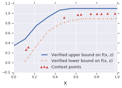
At test time, the neural process is given a new set of context points (pairs of inputs and function values) form a previously unseen CDF and asked to predict the value of the CDF at a set of target points. The context points are plotted as red triangles in figure 1. Our verification is on the prediction of the NP at the unseen target points. We use the verification algorithm to compute bounds on the probability that when the target input is in a given range, the predicted output is above or below a certain bound.

We choose a threshold of $\epsilon=.01$ and find the smallest bound $a$ such that $f\left({x,z}\right)\leq a$ with probability at least $1-\epsilon$ as a function of a range specified on $x$. Specifically, we consider intervals of width $.02$, ie $x\in\mathcal{X}=[\delta,\delta+.02]$ and plot the value of $a$ as a function of $\delta$. Similarly, we find the largest lower bound $b$ such that $f\left({x,z}\right)\geq b$ with probability at least $1-\epsilon$. The upper bound is plotted as a solid blue line, and the lower bound as a dashed yellow line. The results show that the values of $a,b$ increase with $\delta$, and generally conform with the properties of a CDF, thus showing that our verification algorithm is indeed able to prove properties we expect to be true of the model.

We presented a novel verification formulation and algorithm for verification of deep probabilisitc models. In future work, we will study more complex models (CVAEs, GANs), specifications (for example, verifying disentangled representations) and integration of verification into training .

References

- Boyd and Vandenberghe (2004) Stephen Boyd and Lieven Vandenberghe. Convex optimization. Cambridge university press, 2004.
- Bunel et al. (2017) Rudy Bunel, Ilker Turkaslan, Philip HS Torr, Pushmeet Kohli, and M Pawan Kumar. Piecewise linear neural network verification: A comparative study. arXiv preprint arXiv:1711.00455, 2017.
- Dvijotham et al. (2018) Krishnamuthy Dvijotham, Robert Stanforth, Sven Gowal, Timothy Mann, and Pushmeet Kohli. Towards scalable verification of neural networks: A dual approach. In Conference on Uncertainty in Artificial Intelligence, 2018.
- Frazier (2018) Peter I Frazier. A tutorial on bayesian optimization. arXiv preprint arXiv:1807.02811, 2018.
- Garnelo et al. (2018a) Marta Garnelo, Dan Rosenbaum, Chris J Maddison, Tiago Ramalho, David Saxton, Murray Shanahan, Yee Whye Teh, Danilo J Rezende, and SM Eslami. Conditional neural processes. arXiv preprint arXiv:1807.01613, 2018a.
- Garnelo et al. (2018b) Marta Garnelo, Jonathan Schwarz, Dan Rosenbaum, Fabio Viola, Danilo J Rezende, SM Eslami, and Yee Whye Teh. Neural processes. arXiv preprint arXiv:1807.01622, 2018b.
- Katz et al. (2017) Guy Katz, Clark Barrett, David L Dill, Kyle Julian, and Mykel J Kochenderfer. Reluplex: An efficient smt solver for verifying deep neural networks. In International Conference on Computer Aided Verification, pages 97–117. Springer, 2017.
- Kingma and Welling (2013) Diederik P Kingma and Max Welling. Auto-encoding variational bayes. arXiv preprint arXiv:1312.6114, 2013.
- Sohn et al. (2015) Kihyuk Sohn, Honglak Lee, and Xinchen Yan. Learning structured output representation using deep conditional generative models. In Advances in Neural Information Processing Systems, pages 3483–3491, 2015.
- Van Den Oord et al. (2016) Aaron Van Den Oord, Sander Dieleman, Heiga Zen, Karen Simonyan, Oriol Vinyals, Alex Graves, Nal Kalchbrenner, Andrew Senior, and Koray Kavukcuoglu. Wavenet: A generative model for raw audio. arXiv preprint arXiv:1609.03499, 2016.
- Weng et al. (2018) Tsui-Wei Weng, Huan Zhang, Hongge Chen, Zhao Song, Cho-Jui Hsieh, Duane Boning, Inderjit S Dhillon, and Luca Daniel. Towards fast computation of certified robustness for relu networks. arXiv preprint arXiv:1804.09699, 2018.
- Xu et al. (2015) Kelvin Xu, Jimmy Ba, Ryan Kiros, Kyunghyun Cho, Aaron Courville, Ruslan Salakhudinov, Rich Zemel, and Yoshua Bengio. Show, attend and tell: Neural image caption generation with visual attention. In International conference on machine learning, pages 2048–2057, 2015.