On Min-Max affine approximants of convex or concave real valued functions from $\mathbb{R}^{k}$, Chebyshev equioscillation and graphics.

We will work in ${\mathbb{R}}^{k},k\geq 1$ where ${\bf x}\in{{\mathbb{R}}^{k}}$ is the column vector $[x_{1}\,x_{2}\,\cdots\,x_{k}]^{T}$ and $T$ denotes transpose. A function $g:{{\mathbb{R}}^{k}}\rightarrow{\mathbb{R}}$ is an affine function provided there exists ${\bm{\alpha}}\in{{\mathbb{R}}^{k}},\,{\rm and}\,\beta\in{\mathbb{R}}$ such that $g({\bf x})={\bm{\alpha}}^{T}{\bf x}+\beta$.

Our main result is

Theorem 2.1 belongs to an interesting class of related optimization problems which can be found for example in ANW; Br; Da; D; Korn; L; Mir; Nik; Tem.

We know of no convex domain other than a $k$-simplex where we can generate a hyperplane $\pi$ as in Theorem 2.1 for which we can verify that the graph of $f$ over the domain lies entirely above or entirely below that hyperplane.

We now present two remarks regarding Theorem 2.1.

The key ideas in our proof of Theorem 2.1 are the two equivalent definitions of a convex function. $f:\Delta\subset\mathbb{R}^{k}\to\mathbb{R}$ is convex provided $\textnormal{for all }\gamma_{i}\geq 0:\Sigma_{i=1}^{k+1}\gamma_{i}=1,$ and any affine independent set of $k+1$ points $\{{{\bf a}}^{\prime}_{1},\ldots,{{\bf a}}^{\prime}_{k+1}\}$, $f(\Sigma_{i=1}^{k+1}\gamma_{i}{{\bf a}}^{\prime}_{i})\leq\Sigma_{i=1}^{k+1}\gamma_{i}f({{\bf a}}^{\prime}_{i})$, i.e. the graph of $f$ over the convex hull of $k+1$ affinely independent points lies below the convex hull of the $k+1$ image points $\{[{{\bf a}}^{\prime}_{i}{}^{T}\,\,f({{\bf a}}^{\prime}_{i})]^{T}:1\leq i\leq k+1\}$, or equivalently, $\textnormal{for each }{\bf x}\in\Delta,$ $\textnormal{and each support plane at }[{\bf x}^{T}\,\,f({\bf x})]^{T}$ $\textnormal{ with slope }{\bf\eta}\in{\mathbb{R}}^{k}$, $f({\bf y})\geq f({\bf x})+{\bf\eta}^{T}({\bf y}-{\bf x}),$ $\textnormal{for all }{\bf y}\in\Delta$, i.e. the graph of $f$ lies on or above any supporting hyperplane.

For our proof of Theorem 2.1, we advise the reader to use Figure 1 for intuition.

Note that even if $f$ is not convex (or concave) and not even smooth the method produces a best uniform approximation for the $k+2$ points comprised of the $k+1$ points $({\bf a}_{1},f({\bf a}_{1}))\ldots,({\bf a}_{k+1},f({\bf a}_{k+1}))$ and $({\bf y},f({\bf y}))$.

For $k=1$, our main result Theorem 2.1 provides an extension of the classical Chebyshev equioscillation theorem, see Theorem 4.1 below, for linear approximants with an explicit unique formula for the best approximant.

We now explain this.

One consequence of Theorem 2.1 gives an interesting connection to graphics. We provide our ideas below.

We are given a flat object $\mathcal{O}$ and want to render it from a given perspective, camera setup. The resulting image is a projective (AKA perspective or homography) transformation of $\mathcal{O}$, $P(\mathcal{O})$. Thus, each pixel (color) in $\mathcal{O}$, (an ordered pair $(x_{1},y_{1})$ in $\mathbb{R}^{2}$) is transformed to a new pixel location (point) 2 via the action of $P$

Practically, to render this object which can have 10’s of millions of pixels it is useful to have a good fast approximation of the transformation not entailing division which can cause numerical instabilities. Thus, we seek affine approximants to $P$. One known method is to simply take the affine approximant to be the linear terms of the Taylor expansion around one point, the tangent approximation.

We aim to provide a better 2d-affine approximant to $P$ than the tangent approximation. From Equation 5.1 the components of $P({\bf x})$ are given by

From our main Theorem 2.1 we know that if we can find a triangle, $\Delta$, containing (a large part of) $\mathcal{O}$ such that each $f_{i}({\bf x})$ is convex or concave then there exist Min-Max affine approximations ${{\bm{\alpha}}_{i}}^{T}{\bf x}+\beta_{i}$ to each $f_{i}$. Then forming the affine transformation $A$ of 2-space given by

provides, component wise, the best uniform affine approximants on $\Delta$.

Since a differentiable function is convex or concave on a domain exactly when it’s Hessian is respectively positive or negative semidefinite the following is a key tool for the application of our main result.

The Hessian of

is

with determinant $\frac{-\beta^{2}}{(X+\delta)^{4}}$. The sign of $H[1,1]=2(\beta Y-\alpha\delta+\gamma)$ depends on $Y\begin{matrix}<\\ >\end{matrix}\frac{\alpha\delta-\gamma}{\beta}$.

When we combine Proposition 5.1 with the Hessian of Eq. 5.4 we see that $\frac{\alpha X+\beta Y+\gamma}{X+\delta}$ in each of the connected components of ${\mathbb{R}}^{2}\setminus\{\{X=-\delta\}\cup\{Y=\frac{\alpha\delta-\gamma}{\beta}\}\}$ is either convex or concave. With the 2 coordinate functions of the projective transformation ($X$ and $Y$) we end with 6 regions in ${\mathbb{R}}^{2}$ where Theorem 2.1 holds, Figure 2.

In order to transform a general projective transformation as in Eq.  5.3 to the form in Eq. 5.4, with a simple denominator, we rotate the axes so that $X$ is in the direction of $\begin{bmatrix}d\\ e\end{bmatrix}$ and normalize so that the coefficient of $X$ in the denominator is 1.

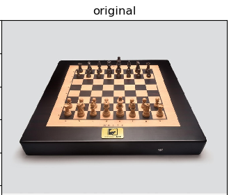
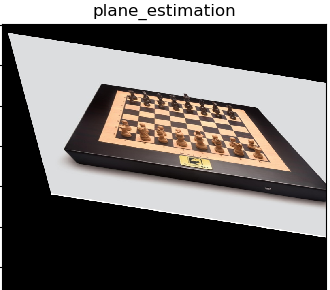
In Figure 3 we show a few examples of the various affine approximations $A$ of projective transformations $P$ using this idea.

The first column is the original image $\mathcal{O}$, the second column is the image transformed by a projective transformation $P$, modelling a new viewpoint, the third column is the transformation based on the affine approximation $A$ of $P$ using Theorem 2.1 and a user defined triangle while the fourth column is computed using a Taylor series approximation of $P$ around the image’s center. The images in column 3 should visually look closer to those in column 2 than those in column 4, the Taylor approximation.

References

- (1) J.H. Ahlberg, E.N. Nilson, J.F. Walsh, Theory of splines and their applications, Acad. Press (1967).
- (2) Y.A. Brudnyi, Approximation of functions defined in a convex polyhedron, Soviet Math. Doklady, 11. 6 (1970), (pp. 1587-1590), Dokl. Akad. Nauk SSSR, 195 (1970), (pp. 1007-1009).
- (3) P.J. Davis, Interpolation and approximation, New York, 1963.
- (4) F. Deutsch, Best approximation in inner product spaces, CMS Books in Mathematics, 2001.
- (5) M. Krein, A. Nudelman, The Markov Moment problem and extremal problems, AMS translation from the Russian edition of 1973.
- (6) N.P. Korneichuk, Extremal problems in approximation theory , Moscow (1976) (In Russian).
- (7) P.J. Laurent, Approximation et optimization, Hermann (1972).
- (8) V.L. Miroshichenko, Methods of spline functions, Moscow (1980).
- (9) S.M. Nikol’skii, Approximation of functions of several variables and imbedding theorems, Springer (1975) (Translated from Russian).
- (10) L. Schumaker, Spline Functions: basic theory, Academic Press, NY, 1983.
- (11) V.N. Teml’yakov, Best approximations for functions of two variables, Soviet Math. Doklady, 16: 4 (1975), (pp. 1051-1055), Dokl. Akad. Nauk SSSR, 223 (1975), (pp. 1079-1082).